Abstract
Gait pattern generation has an important influence on the walking quality of biped robots. In most gait pattern generation methods, it is usually assumed that the torso keeps vertical during walking. It is very intuitive and simple. However, it may not be the most efficient. In this paper, we propose a gait pattern with torso pitch motion (TPM) during walking. We also present a gait pattern with torso keeping vertical (TKV) to study the effects of TPM on energy efficiency of biped robots. We define the cyclic gait of a five-link biped robot with several gait parameters. The gait parameters are determined by optimization. The optimization criterion is chosen to minimize the energy consumption per unit distance of the biped robot. Under this criterion, the optimal gait performances of TPM and TKV are compared over different step lengths and different gait periods. It is observed that (1) TPM saves more than 12% energy on average compared with TKV, and the main factor of energy-saving in TPM is the reduction of energy consumption of the swing knee in the double support phase and (2) the overall trend of torso motion is leaning forward in double support phase and leaning backward in single support phase, and the amplitude of the torso pitch motion increases as gait period or step length increases.
1. Introduction
Compared with other types of robots, humanoid robots have good adaptability to the environment, strong obstacle avoidance ability, small moving blind area, and good quality in line with human habits. These have attracted great attention and in-depth research of scholars, such as dynamics analysis [1,2,3], stability criteria [4,5,6], trajectory planning [7,8,9,10], etc. Because the development of humanoid robots is restricted by the development of mechanism, materials, computer technology, control technology, microelectronics technology, communication technology, sensor technology, artificial intelligence, mathematical methods, bionics, etc., humanoid robots cannot yet achieve real anthropomorphism. There are still many problems to be solved in this field, such as walking stability, high-speed walking, reducing energy consumption, etc.
Gait is a type of coordination relationship between joints in time and/or space when a robot is walking. Gait planning of biped robots depends on the ground conditions, lower limb structure, and the control difficulty, and it must meet the requirements of motion stability, walking speed, mobility, etc. For this reason, a variety of methods for gait planning have been adopted.
Gait planning methods based on a simplified model are commonly used methods, such as an inverted pendulum or linear inverted pendulum [11,12]. The simplified model brings a lot of convenience to robot research. The state of the system is only the position and velocity of the center of mass (CoM) of the robot. The gait is generated by the motion of CoM and the design of the landing point, and the trajectory of each join is obtained by inverse kinematics. The disadvantage is that the simplified model is an approximation of the robot and it is not accurate enough. When studying the energy efficiency of biped walking, this in-accurate model is difficult to work on.
The method based on the zero-moment point (ZMP) stability criterion is another common method of gait planning. This type of method designed the reference ZMP trajectory first and then determined the motion of each joint that can realize the reference ZMP trajectory. Kajita et al. [13] and Dasgupta et al. [14] used ZMP based stability criteria to generate gait patterns. The advantage of this method is that if the reference ZMP is designed near the center of the stable region, the stability margin can be large. However, due to the limited changes of ZMP caused by hip motion, not all the expected ZMP trajectories can be achieved. In addition, in order to obtain the desired ZMP trajectory, the hip joint acceleration may need to be very large. In this case, due to the relatively large torso, energy consumption increases, and it is difficult to control the upper body.
There are also some methods based on the multi-link model. Mu et al. [15], Song et al. [16], and Ghiasi et al. [17] designed the gait pattern of a five-link biped robot, and Farzadpour et al. [9] and Fattah et al. [18] designed the gait pattern of a seven-link biped robot. In their methods, the trajectories of hip and feet were defined in different ways first, then joint angles were obtained by inverse kinematics. In addition, torso angle was designed vertical during walking in their methods. This may make the design of the torso angle simple. However, torso keeping vertical may not be the best energy-efficient method for biped walking.
This paper presents a gait generation method for biped robots with torso pitch motion (TPM). We also provide a common gait pattern with torso keeping vertical (TKV) to study the effects of TPM on the energy efficiency of biped robots. Based on the model of a planar five-link robot, the gait of the biped robot is generated by optimization. Firstly, the trajectories of hip position, torso angle, swing ankle position are designed as polynomials with some gait parameters. Then, the minimum total energy consumed by the joint actuators per unit distance is chosen as the optimization objective, and the gait parameters are determined by optimization. Finally, two sets of optimal gaits with different gait periods and different step lengths are generated.
The main contributions of this paper are as follows:
- (1)
- Propose a gait pattern generation method for biped robots with the torso pitch motion, define the cyclic gait of a biped robot with multiple gait parameters, choose the minimum total energy consumed by the joint actuators per unit distance as the optimization objective, and determine the gait parameters by optimization;
- (2)
- Generate the optimal gait of TPM and TKV for different step lengths and different gait periods and compare the energy consumption of the two gait patterns; the optimization results show that TPM is over 12% more energy-efficient than TKV;
- (3)
- Carry out parameter study. Although the parameters related to the torso motion with different gait periods and step lengths are various, the overall trend is that torso leans forward during the double support phase (DSP) and leans backward during the single support phase (SSP);
- (4)
- Compare the energy consumption of each joint and observe that the main factor of energy-saving in TPM compared with TKV is the reduction of energy consumption of the swing knee during DSP.
The structure of the rest of this paper is as follows: The second section introduces the modeling of biped robots. In the third section, some gait parameters are designed to define the trajectories. Then, in the fourth section, the optimization of gait parameters is discussed. The optimization results of the optimal gait and the comparison between TPM and the TKV are given and discussed in the fifth section. Finally, the sixth section summarizes the paper.
2. Biped Robot Modeling
2.1. Biped Robot Model
Because the main movements of biped robots take place in the sagittal plane during walking, this paper only considers the 2D model. A five-link planar biped robot with knees can capture most of the features of biped walking. Therefore, we choose a five-link planar biped robot model and plan its walking gait. The robot’s five links include a torso, two thighs, and two shanks. The five links are connected by four revolute joints—two hips and two knees. Each joint has an actuator. Assume that each link is rigid and each joint is frictionless. In addition, we neglect two feet to simplify the model because the mass of each foot of the robot is relatively light. However, we should keep in mind that there is a finite size foot at the tip of each leg. Hence, torque is applied at the stance ankle. The geometric dimensions of the robot are shown in Figure 1 in which and represent the mass and length of link-i, respectively; represents the distance from the center of mass (CoM) of link-i to its lower joint; and represents the moment of inertia of link-i about the axis passing through the CoM of link-i and perpendicular to the sagittal plane.
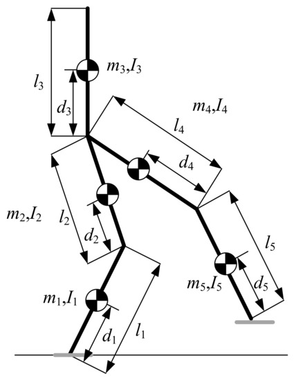
Figure 1.
Biped robot model with massless feet.
2.2. Walking Cycle
The cyclic gait planned in this paper includes DSP and SSP, as shown in Figure 2. The current step is from the beginning of DSP to the end of SSP. At the moment t = 0, foot-1 lands on the ground in front of foot-2, the DSP begins. At the moment , foot-2 takes off the ground, the DSP ends and the SSP begins simultaneously. During the SSP, foot-2 swings from the back of foot-1 to the front of foot-1. At the moment , the SSP ends and the current step also completes when foot-2 lands in front of foot-1. Then, the next step begins simultaneously and the two legs exchange their roles. The gait period of one step is , the duration of DSP is , and the duration of SSP is . In order to reduce the impact of swing foot landing and obtain a DSP after impact, we assume that the velocity of the swing foot is equal to zero at its landing [19].
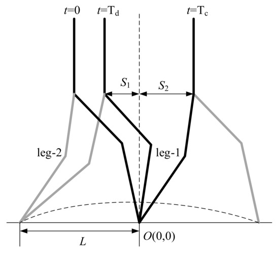
Figure 2.
Walking cycle including double support phase (DSP) and single support phase (SSP). Origin of world frame is at the stance ankle. L is the step length, and S1 and S2 are the hip horizontal positions at the beginning and at the end of SSP, respectively.
2.3. Motion Equations
Generally, seven degrees of freedom are needed to describe a five-link planar biped robot. However, according to the definition of the walking cycle in Section 2.2, foot-1 always keeps contact with the ground and does not slip in the current step; hence, the biped robot can be regarded as a rooted system. Therefore, the generalized coordinates can be described as (see Figure 3). A coordinate frame is attached to the flat ground called the world frame, its origin is at the ankle of foot-1. In addition, counterclockwise is the positive direction of the angle. In this paper, we assume the biped robot walks from left to right on level ground.
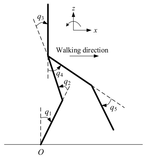
Figure 3.
Generalized coordinates of the five-link biped model. The x-direction is the walking direction and the z-direction is the upright direction, angles are measured by counterclockwise direction.
Based on Lagrange’s formula, the motion equation of SSP is written as the following compact form:
where M is symmetric and positive defined inertia matrix, C is the matrix related to centrifugal and Coriolis terms, G is the vector of gravity terms, is the vector of actuated joint torques, and B is a constant matrix composed of ones and zeros representing the contribution of the actuated joint torques.
During the DSP, it can be considered that foot-2 is constrained on the basis of the motion equation of the SSP. The constraint equation can be expressed as
where the additional constraints and are the horizontal and vertical positions of the ankle of foot-2, respectively; L is the step length as shown in Figure 2. The motion equation of the DSP is
where is the constrained Jacobian matrix, is the Lagrange multiplier.
3. Trajectory Planning
If the hip trajectory and ankle trajectories are known, all joint angles of the biped can be obtained by inverse kinematics. Hence, gait patterns can be denoted uniquely by the hip trajectory and ankle trajectories if the knees of the biped bend forward similar to human beings. To this end, we plan the hip and ankle trajectories by polynomials. In this section, we design two gait patterns, TPM and TKV, for our study. The only difference between the two gait patterns is the torso pitch motion.
The duration of DSP or SSP is an important parameter in biped walking. If the duration of DSP is too short, the ZMP must be transferred from the trailing foot to the leading foot in a very small time. If the duration of the DSP is too long, it is difficult to walk at a high speed. In the study of human walking, it is observed that the time interval of DSP is about 20% of one step’s duration [20]. Therefore, in this paper, we specify that the duration of the DSP accounts for 20% of the walking cycle, that is, .
3.1. Trajectory of the Swing Ankle
During DSP, the swing ankle also remains constant with respect to the floor, and hence its displacements in the horizontal and vertical directions are
During SSP, the trajectory of the swing ankle can be described as a certain order polynomial that satisfies some constraints. To plan the trajectory of the swing ankle during SSP, three specific positions are taken into consideration. The first is the ankle position at the beginning of SSP, the second is the ankle position at the end of SSP, and the last is the ankle’s highest position. Therefore, the horizontal and vertical trajectories of swing ankle are designed as
respectively. Constant polynomial coefficients (i = 0,1,2,3) are determined by the following boundary conditions:
Constant polynomial coefficients (i = 0,1, …, 5) are determined by the following boundary conditions:
where is the maximum height of swing ankle at time during SSP. In this research, we set = 0.1 m and .
3.2. Trajectory of the Hip
Hip horizontal trajectories in DSP and SSP are designed as two third-order polynomials, respectively.
The hip trajectory should be continuous during the walking step. Therefore, the displacement and velocity of the hip at the end of DSP should be equal to those at the beginning of SSP. Furthermore, to keep ZMP continuous, the acceleration of the hip is also required to be continuous. Thus, the following continuity condition should be satisfied:
where is the hip position with respect to stance ankle in the horizontal direction at the end of DSP, as shown in Figure 2.
To keep the gait repeatable, the configuration at the beginning of DSP should be identical to the one at the end of SSP and the velocity of the hip at the beginning of DSP should be the same as the one at the end of SSP. In addition, to make the motion smooth, the acceleration of the hip at the beginning of DSP should be equal to the one at the end of SSP. Therefore, the following cyclic condition should be satisfied:
where is the hip position with respect to stance ankle in the horizontal direction at the end of SSP, as shown in Figure 2.
Constant polynomial coefficients and (i = 0, 1, …, 3) are determined by Equations (12) and (13), respectively.
In this paper, hip vertical motion is not our focus. Therefore, hip height keeps unchanged during walking. The trajectory of is described as follows:
where H is also a design parameter that will be determined by optimization.
3.3. Torso Angle
3.3.1. TKV
In the traditional method, the torso keeps vertical during walking. Therefore, the trajectory of torso angle is
3.3.2. TPM
The absolute angle of the torso is the angle between the torso and the vertical direction, which is positive in the counterclockwise direction. When the biped robot walks periodically, its torso angle also makes a periodic motion. We design this torso angle trajectory as follows: its angle is at the switching time of SSP and DSP, reaches an extreme value at the middle time of DSP, and reaches an extreme value at the middle time of SSP. In other words, torso angle is at the beginning of DSP, reaches the extreme value at the middle of DSP and then returns to the angle at the end of DSP; the torso angle is at the beginning of SSP, reaches the extreme value at the middle of SSP and then returns to at the end of SSP. According to the continuity and smoothness of torso motion, we can know that the value of is between and . However, we do not know which one is bigger in and . , , and are gait parameters that will be determined by optimization. The absolute angles of the torso are designed as two fifth-order polynomials in DSP and SSP, respectively.
At first, torso motion should be continuous and smooth in a gait step. Therefore, the following continuity conditions should be satisfied:
Secondly, the following cyclic conditions should be satisfied:
Lastly, the extremum conditions for DSP and SSP are the follows:
The polynomial coefficient and (i = 0, 1, …, 5) is determined by Equations (18)–(20).
4. Optimization Problem
In this section, an optimization problem is proposed to determine the gait parameters. Section 4.1 yields the objective function of the optimization, and Section 4.2 results in the constraints of optimization. To calculate the objective function, joint torques need to be calculated. To calculate joint torques using dynamic Equation (1), however, one should first calculate joint angles, angular velocities, and angular accelerations. Therefore, Section 4.3 introduces how to calculate the joint angles, angular velocities, and angular accelerations. Section 4.4 introduces how to calculate joint torques for DSP and SSP.
4.1. Objective Function
Energy consumption is a key criterion to evaluate the performance of the robot. The less the energy is consumed, the farther the biped robot can travel. Therefore, in this study, the optimization objective is to minimize energy consumption per unit distance of biped robots. The objective function is described as
with nonlinear constraints and bounded condition as follows:
where x is the vector of optimization variables.
4.2. Optimization Constraints
We use the ZMP criterion to ensure the robot’s stability. The ZMP can be calculated using the following equation [8]:
where is the mass of link-i; and are the horizontal and vertical position of CoM of link-i, respectively; is the inertia of link-i about its CoM; is the absolute angle of link-i; and g is the gravitational constant.
During the optimization process, the ZMP criterion should be satisfied. Accordingly, the optimization inequality constraints will be
where and are the ZMP margins in the stance foot specified by users, which are not necessarily equal to the horizontal position of stance heel and toe with respect to stance ankle, respectively. In addition, the distance between hip and ankle should be less than leg length; otherwise, the angle of the knee joint cannot be solved by inverse kinematics. Therefore, the following inequality constraints should also be satisfied:
where is the distance from the hip to the ankle of the support leg and is the distance from the hip to the ankle of the swing leg.
4.3. Angles, Angular Velocities, and Angular Accelerations
In Section 3, trajectories of hip position, torso angle, swing ankle position have been defined. Then knee angles can be calculated using inverse kinematics when the related ankle position and hip position are known. In this paper, we do not use a numerical solution method but an analytical solution method to calculate joint angles. According to the geometric relationship, one can obtain the joint angles as follows:
where , and is the virtual length of stance leg; , and is the virtual length of the swing leg.
Next, we introduce how to calculate angular velocity and angular acceleration. Define a vector whose components were defined in Section 3. According to the kinematic relationship, can be expressed in terms of . Its derivative with respect to time is
where is the Jacobian matrix and it is invertible. Therefore, angular velocity can be calculated as follows:
Differentiating Equation (27) once more yields
Then, one can obtain angular accelerations as follows:
4.4. Joint Torques
After knowing the generalized coordinates, velocities, and accelerations, one can calculate the joint torques by inverse dynamic equations.
In SSP, it is quite easy to obtain the joint torques using Equation (1) because matrix B is an identity matrix in the case of chosen generalized coordinates.
In DSP, the biped robot model has three degrees of freedom and five independent actuators; therefore, it is over-actuated. For a given state and acceleration, the solutions of joint torques are not unique. Let be the constraint forces compatible with constraints (2). By using the constraints (2), the joint torques and constraint forces can be derived. To this end, generalized coordinates can be divided into two parts—unconstrained coordinates and constrained coordinates . We can denote this as
where is an invertible constant matrix that rearranges the components of vector . By deriving the constraint Equation (2), we can obtain
where and are submatrices of . With appropriate choice of and , could be an invertible matrix. Thus, one can obtain
where is
and is an identity matrix.
Multiplying dynamic Equation (3) by from the left-hand side and noticing , one can obtain
Note that Equation (35) has three equations but five unknowns . Therefore, the dynamics system is over-actuated during DSP, and the solution of Equation (35) is not unique. In this study, among all solutions, we specify the solution that has the least sum of squares.
where and is the pseudo-inverse matrix of .
5. Simulation Results and Discussion
In this section, the trajectory of a five-link biped robot with SSP and DSP is simulated. The physical parameters corresponding to the five-link model are the robot prototype developed in our laboratory. The prototype is about 1.57 m high, with a total mass of 40 kg and 23 degrees of freedom. The physical parameters of the robot are listed in Table 1.

Table 1.
Physical parameters of the biped model.
For a complex nonlinear optimization problem, it is usually difficult to guarantee the solution solved is the global optimal solution. In order to get a convincing optimal solution, we first use a genetic algorithm to solve each optimization problem and get several solutions and then use the sequential quadratic program (SQP) algorithm to solve each optimization problem again with these solutions as initial values. The optimization results show that the same results are obtained by the SQP algorithm with different initial values obtained by the genetic algorithm. Therefore, the solution can be considered as the global optimal solution.
5.1. Simulation Results of TPM
The following shows the details of TPM when the step length is 0.3 m and the gait period is 1.0 s.
Figure 4 shows the angle trajectory of each joint, and Figure 5 shows the angular velocity trajectory of each joint. It can be seen that the joint angle is smooth and the joint angular velocity is continuous. However, the angular velocity is not smooth when switching from DSP to SSP. This means that the angular acceleration is not continuous at this moment, because the ankle of the swing leg starts to lift at that time, and its acceleration is not continuous. Similarly, the joint angular acceleration is also discontinuous when the SSP is switched to the next DSP because the acceleration of the swing ankle is discontinuous at that moment.
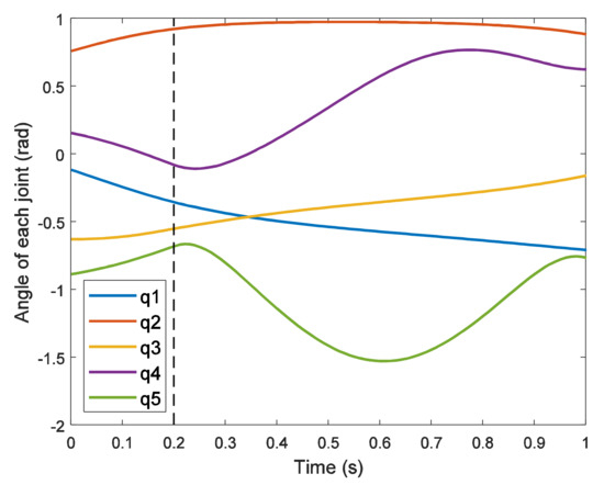
Figure 4.
Angle trajectories.
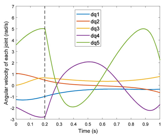
Figure 5.
Trajectories of angular velocities.
Figure 6 shows the trajectories of joint torques. In DSP, because the system is over- actuated, the number of independent actuators is greater than the degrees of freedom; therefore, the driving torque of the two joints is released, and only are actuated. In SSP, we can see that the driving torque of the knee joint of the support leg is much larger than that of the other joints. It plays the role of support the whole upper body and swing leg.
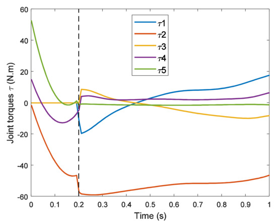
Figure 6.
Torque trajectories.
According to the planned gait and the dynamic equation, the ground reaction force on the robot foot can be obtained, as shown in Figure 7, where is the ground reaction force (GRF) on support foot, is the GRF on swing foot. It is observed from Figure 7 that (1) the swing foot is only subjected to the ground reaction during the DSP; (2) the normal component of the GRF is positive, which ensures the unilateral constraint characteristics of the GRF; (3) the tangential component of the GRF is much smaller than the normal component of GRF, which ensures no sliding between the foot and the ground; and (4) during SSP, the normal component of the GRF applied on the support foot is approximately equal to the gravity of the robot (about 400 N).
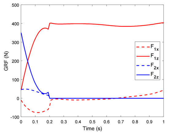
Figure 7.
Trajectories of ground reaction force (GRF).
Figure 8 shows the ZMP trajectory and the upper and lower boundaries of the ZMP in one step. The stability margin of ZMP is = 0.1 m, = 0.05 m, while the horizontal distance from ankle to toe is 0.13 m and the horizontal distance from ankle to heel is 0.07 m. It can be seen from the figure that ZMP is within the stability margin, which ensures the stability of the walking.
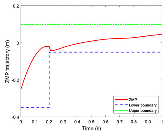
Figure 8.
Trajectory of ZMP.
Figure 9 shows the stick diagram of the five-link robot walking on the horizontal ground, in which the dashed line represents the DSP, and the solid line represents the SSP. From the stick diagram, we can observe the overall movement of the biped robot, i.e., that the posture at the end of each step is the same as that at the beginning of each step.
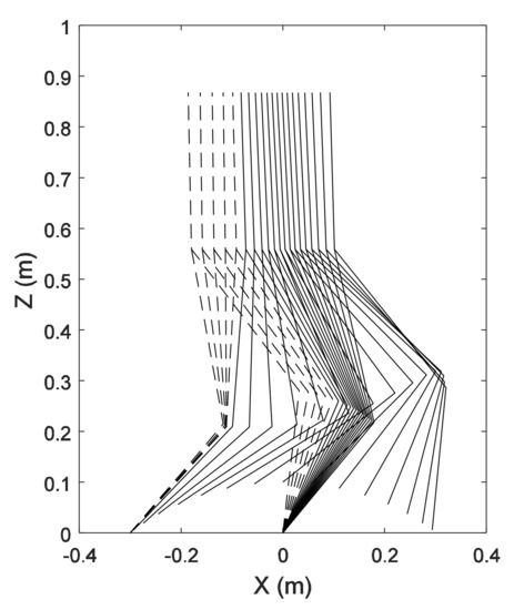
Figure 9.
Stick diagram of one step.
Generally, the gait pattern designed by the proposed method is simple and easy to implement. Although the contact constraint between the ground and the foot is not considered in the gait generation, the simulation results verify that the friction force is very small relative to the support force during walking. Therefore, the biped robot can walk without sliding even if the friction coefficient between the foot and the ground is small.
5.2. Comparison of TPM and TKV on Energy Consumption
On the one hand, to study the relationship between gait period and walking efficiency, we fix the step length and change the gait period. In this research, we specify a fixed step length L = 0.3 m, and gait period changes from 0.7 s to 1.2 s. Figure 10 shows the energy consumption in this case.
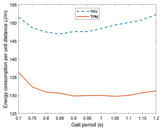
Figure 10.
Energy consumption of two gait patterns with different gait periods when L = 0.3 m.
From simulation results, we can obtain the following observations:
- (1)
- The energy consumption per unit distance of TPM is less than that of TKV. When the step length is 0.3 m and the gait period changes from 0.7 s to 1.2 s, the energy consumption per unit distance of TPM is about 12.14% less than that of TKV on average;
- (2)
- The optimal period of TKV is 0.85–0.95 s, while that of TPM is 0.9–1.1 s. The effect of the period change of TPM on energy consumption is smaller than that of TKV, except for 0.7 s and 0.75 s.
On the other hand, to study the relationship between step length and energy consumption, we fix the gait period and changed step length. In this research, we specify a fixed period of = 1.0 s, and step length changes from 0.2 m to 0.4 m. Figure 11 shows the energy consumption in this case.
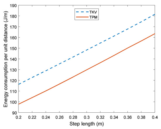
Figure 11.
Energy consumption of two gait patterns with different step lengths when Tc = 1.0 s.
From simulation results, we can obtain the following observations:
- (1)
- The energy consumption per unit distance of TPM is less than that of TKV. When the gait period is 1.0 s and step length changes from 0.2 m to 0.4 m, the energy consumption per unit distance of TPM is about 12.61% less than that of TKV on average;
- (2)
- With the increase of step length, the energy consumption per unit distance of both gait patterns increases. This is consistent with our intuition. When humans walk in larger stride, they are more likely to feel tired.
5.3. Torso Angle Parameters
Figure 12 shows the change of torso angle parameters when the step length remains 0.3 m and the gait period changes from 0.7 s to 1.2 s. We can derive that is always less than . It shows that there is a trend of leaning forward in DSP and leaning backward in SSP. With the increase of the gait period, the amplitude of the torso pitch motion increases. In addition, the three angle parameters are all positive. This is contrary to the intuition that the torso should lean forward. The reason may be to meet the requirements of ZMP stability.
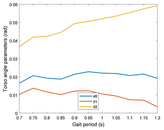
Figure 12.
Torso angle parameters of torso pitch motion (TPM) with different gait periods when L = 0.3 m.
Figure 13 shows the change of torso angle parameters when the gait period remains 1.0s and the step length changes from 0.2 m to 0.4 m. We can derive that is always less than . It also shows that there is a trend of leaning forward in DSP and leaning backward in SSP. With the increase of the step length, the amplitude of the torso pitch motion increases. When the step length is greater than or equal to 0.36 m, the parameter is negative.
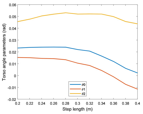
Figure 13.
Torso angle parameters of TPM with different step lengths when Tc = 1.0 s.
5.4. Energy Consumption of Each Joint
From the above discussion, we have observed that the total energy consumption per unit distance of TPM is less than that of TKV. However, we do not obtain any information on the energy consumption of each joint actuator. To this end, we illustrate energy consumption of each joint for two gait patterns with = 1.0 s and L = 0.3 m, as shown in Figure 14. Energy consumptions of support ankle joint and support hip joint of TPM are basically the same as these of TKV. Energy consumptions of the support knee joint and swing hip joint of TPM are a little more than these of TKV. However, the energy consumption of the swing knee joint of TPM is much less than that of TKV. The energy consumption of the swing knee joint is mainly in DSP (see Figure 6). In DSP, the trailing leg (swing leg) pushes the ground to compensate for the energy loss of the previous swing foot landing. As a result, torso pitch motion can reduce the push force of the trailing leg during DSP. This view can also be seen in Figure 15, which shows the ground reaction on the trailing leg for TKV and TPM during DSP. It is observed that the vertical force of TPM is obviously less than that of TKV.
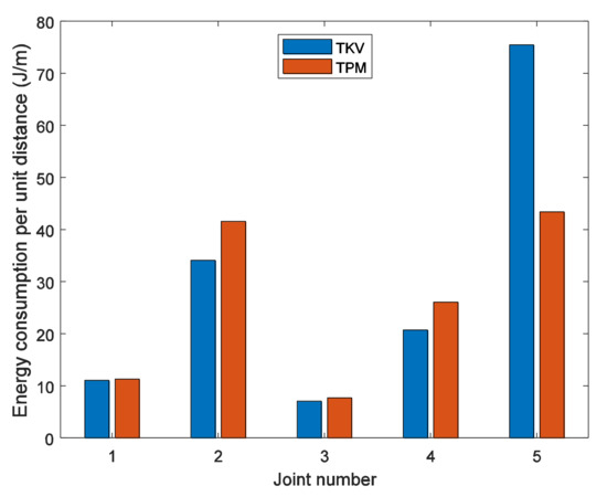
Figure 14.
Energy consumption of each joint when gait period is 1.0 s and step length is 0.3 m.
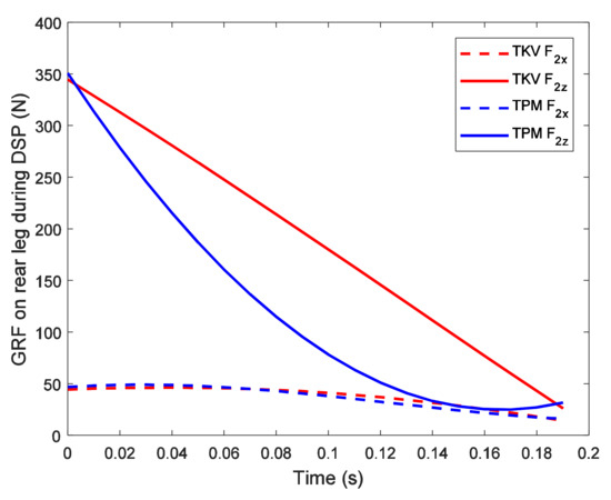
Figure 15.
Ground reaction force on trailing leg during DSP when gait period is 1.0 s and step length is 0.3 m.
6. Conclusions
In this paper, a gait pattern generation method of biped robots with torso pitch motion is proposed to study the influence of torso motion on the walking efficiency of biped robots. The cyclic gait of a five-link biped robot is designed. The trajectories of the hip joint and swing ankle are defined as polynomials. The trajectory of torso angle is also defined as polynomials. The total energy consumption of all joint actuators per unit distance of the robot is chosen as the optimization objective. In addition, a genetic algorithm is used to optimize the gait parameters.
Firstly, a valid walking gait with torso pitch motion can be generated according to our proposed method. As shown in Section 5.1, walking stability is satisfied and ground reaction forces satisfy the unilateral constraints and no-sliding constraints. Secondly, to compare the walking efficiency of TPM and TKV, we generate the optimal gaits with various gait periods and step lengths. According to the optimization results shown in Section 5.2, TPM saves more than 12% energy on average compared with TKV. Thirdly, torso angle parameters are also studied according to optimal gait in Section 5.3. Although the parameters related to the torso motion with different gait periods and step lengths are various, the overall trend is that torso leans forward during DSP and leans backward during SSP. Lastly, in order to analyze the reason that TPM saves energy than TKV, we compare the energy consumption of each joint of TPM and TKV in Section 5.4. It is observed that the main factor of energy-saving in TPM compared with TKV is the reduction of energy consumption of the swing knee during DSP. This is because TPM can reduce the push force of the trailing leg during DSP.
In this research, we designed a gait generation method with TPM that can save more energy than TKV. However, the trajectory of the torso angle we designed is only one of all possible trajectories. There may be a better trajectory for torso angle. This will be the content of our future research.
Author Contributions
Conceptualization, L.L. and X.L.; methodology, L.L. and J.L.; software, L.L.; validation, Z.X. and J.L.; formal analysis, L.L. and Z.X.; investigation, L.L.; writing—original draft preparation, L.L.; writing—review and editing, Z.X. and J.L.; supervision, X.L.; project administration, X.L. All authors have read and agreed to the published version of the manuscript.
Funding
This research was funded by the National Natural Science Foundation of China, grant number 51375085.
Institutional Review Board Statement
Not applicable.
Informed Consent Statement
Not applicable.
Data Availability Statement
No new data were created or analyzed in this study. Data sharing is not applicable to this article.
Acknowledgments
Long Li would gratefully thank Yan Huang at the School of Mechatronics Engineering, Beijing Institute of Technology, for his careful editing of the manuscript and for providing constructive suggestions.
Conflicts of Interest
The authors declare no conflict of interest.
References
- Castano, J.A.; Li, Z.B.; Zhou, C.X.; Tsagarakis, N.; Caldwell, D. Dynamic and Reactive Walking for Humanoid Robots Based on Foot Placement Control. Int. J. Hum. Robot. 2016, 13, 1550041.1–1550041.44. [Google Scholar] [CrossRef]
- Nguyen, Q.; Agrawal, A.; Martin, W.; Geyer, H.; Sreenath, K. Dynamic bipedal locomotion over stochastic discrete terrain. Int. J. Robot. Res. 2018, 37, 1537–1553. [Google Scholar] [CrossRef]
- Luo, X.; Zhu, L.Q.; Xia, L. Principle and method of speed control for dynamic walking biped robots. Robot. Auton. Syst. 2015, 66, 129–144. [Google Scholar] [CrossRef]
- Vukobratovic, M.; Borovac, B. Zero-Moment Point—Thirty five years of its life. Int. J. Hum. Robot. 2004, 1, 157–173. [Google Scholar] [CrossRef]
- Razavi, H.; Bloch, A.M.; Chevallereau, C.; Grizzle, J.W. Symmetry in legged locomotion: A new method for designing stable periodic gaits. Auton. Robot. 2017, 41, 1119–1142. [Google Scholar] [CrossRef]
- Koolen, T.; De Boer, T.; Rebula, J.; Goswami, A.; Pratt, J. Capturability-based analysis and control of legged locomotion, Part 1: Theory and application to three simple gait models. Int. J. Robot. Res. 2012, 31, 1094–1113. [Google Scholar] [CrossRef]
- Gupta, G.; Dutta, A. Trajectory generation and step planning of a 12 DoF biped robot on uneven surface. Robotica 2018, 36, 945–970. [Google Scholar] [CrossRef]
- Huang, Q.; Yokoi, K.; Kajita, S.; Kaneko, K.; Arai, H.; Koyachi, N.; Tanie, K. Planning walking patterns for a biped robot. IEEE Trans. Robot. Autom. 2001, 17, 280–289. [Google Scholar] [CrossRef]
- Farzadpour, F.; Danesh, M.; Torklarki, S.M. Development of multi-phase dynamic equations for a seven-link biped ro-bot with improved foot rotation in the double support phase. Proc. Inst. Mech. Eng. Part C-J. Eng. Mech. Eng. Sci. 2015, 229, 3–17. [Google Scholar] [CrossRef]
- Paparisabet, M.A.; Dehghani, R.; Ahmadi, A.R. Knee and torso kinematics in generation of optimum gait pattern based on human-like motion for a seven-link biped robot. Multibody Syst. Dyn. 2019, 47, 117–136. [Google Scholar] [CrossRef]
- Kajita, S.; Kanehiro, F.; Kaneko, K.; Yokoi, K.; Hirukawa, H. The 3d linear inverted pendulum mode: A simple modeling for a biped walking pattern generation. In Proceedings of the International Conference on Intelligent Robots and Systems (IEEE/RSJ), Maui, HI, USA, 29 October–3 November 2001; pp. 239–246. [Google Scholar]
- Luo, X.; Xu, W.L. Planning and control for passive dynamics based walking of 3D biped robots. J. Bionic Eng. 2012, 9, 143–155. [Google Scholar] [CrossRef]
- Kajita, S.; Kanehiro, F.; Kaneko, K.; Fujiwara, K.; Harada, K.; Yokoi, K.; Hirukawa, H. Biped walking pattern generation by using preview control of the zero moment point. In Proceedings of the IEEE International Conference on Robotics and Automation, Taipei, Taiwan, 14–19 September 2003; pp. 1620–1626. [Google Scholar]
- Dasgupta, A.; Nakamura, Y. Making feasible walking motion of humanoid robots from human motion capture data. In Proceedings of the IEEE International Conference on Robotics and Automation, Detroit, MI, USA, 10–15 May 1999; pp. 1044–1049. [Google Scholar]
- Mu, X.P.; Wu, Q. Synthesis of a complete sagittal gait cycle for a five-link biped robot. Robotica 2003, 21, 581–587. [Google Scholar] [CrossRef]
- Song, B.; Choi, J. Robust Nonlinear Control for Biped Walking with a Variable Step Size. In Proceedings of the SICE-ICASE International Joint Conference, Bexco, Busan, Korea, 18–21 October 2006; pp. 3490–3495. [Google Scholar]
- Ghiasi, A.R.; Alizadeh, G.; Mirzaei, M. Simultaneous design of optimal gait pattern and controller for a bipedal robot. Multibody Syst. Dyn. 2010, 23, 410–429. [Google Scholar] [CrossRef]
- Fakhari, A.; Fattah, A.; Behbahani, S. Dynamics Modeling and Trajectory Planning of a Seven-Link Planar Biped Robot. In Proceedings of the 17th Annual (International) Conference on Mechanical Engineering (ISME), University of Tehran, Tehran, Iran, 19–21 May 2009; pp. 1–7. [Google Scholar]
- Li, L.; Xie, Z.Q.; Luo, X. Impact Dynamics and Parametric Analysis of Planar Biped Robot. In Proceedings of the 25th Inter-national Conference on Mechatronics and Machine Vision in Practice (M2VIP), Stuttgart, Germany, 20–22 November 2018; pp. 97–102. [Google Scholar]
- McMahon, T.A. Muscles, Reflexes, and Locomotion; Princeton University Press: Princeton, NJ, USA, 1984. [Google Scholar]


Publisher’s Note: MDPI stays neutral with regard to jurisdictional claims in published maps and institutional affiliations. |
© 2021 by the authors. Licensee MDPI, Basel, Switzerland. This article is an open access article distributed under the terms and conditions of the Creative Commons Attribution (CC BY) license (http://creativecommons.org/licenses/by/4.0/).