
Design of Road-Side Barriers to Mitigate Air Pollution near Roads


Abstract
:1. Introduction
2. Methodology
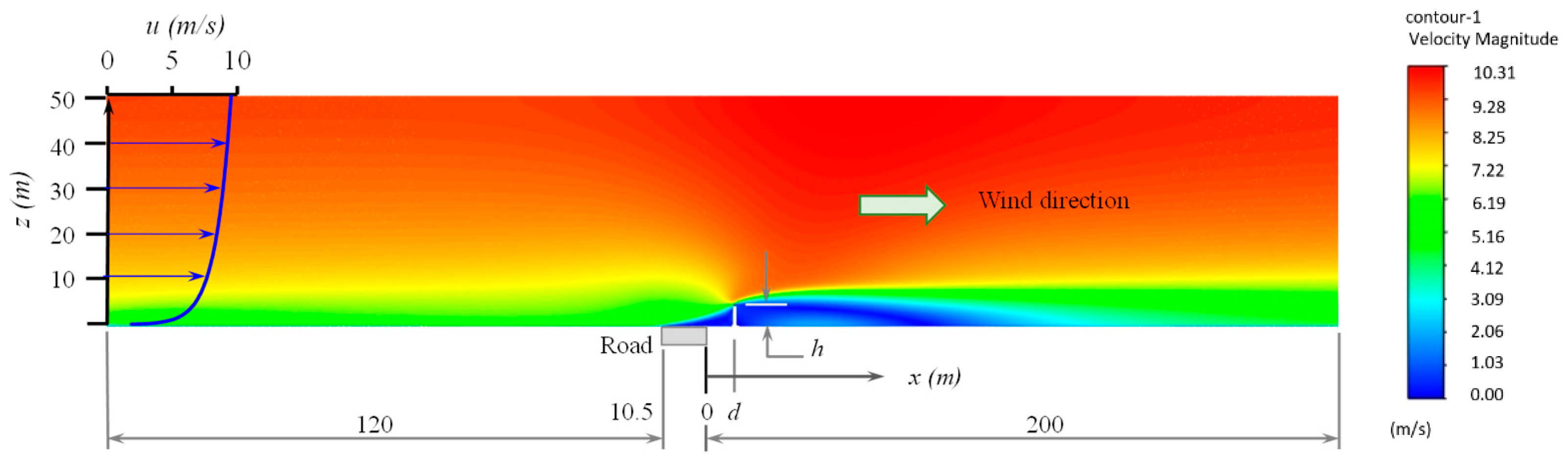
2.1. Case of Study
2.2. Barrier Configuration and Location
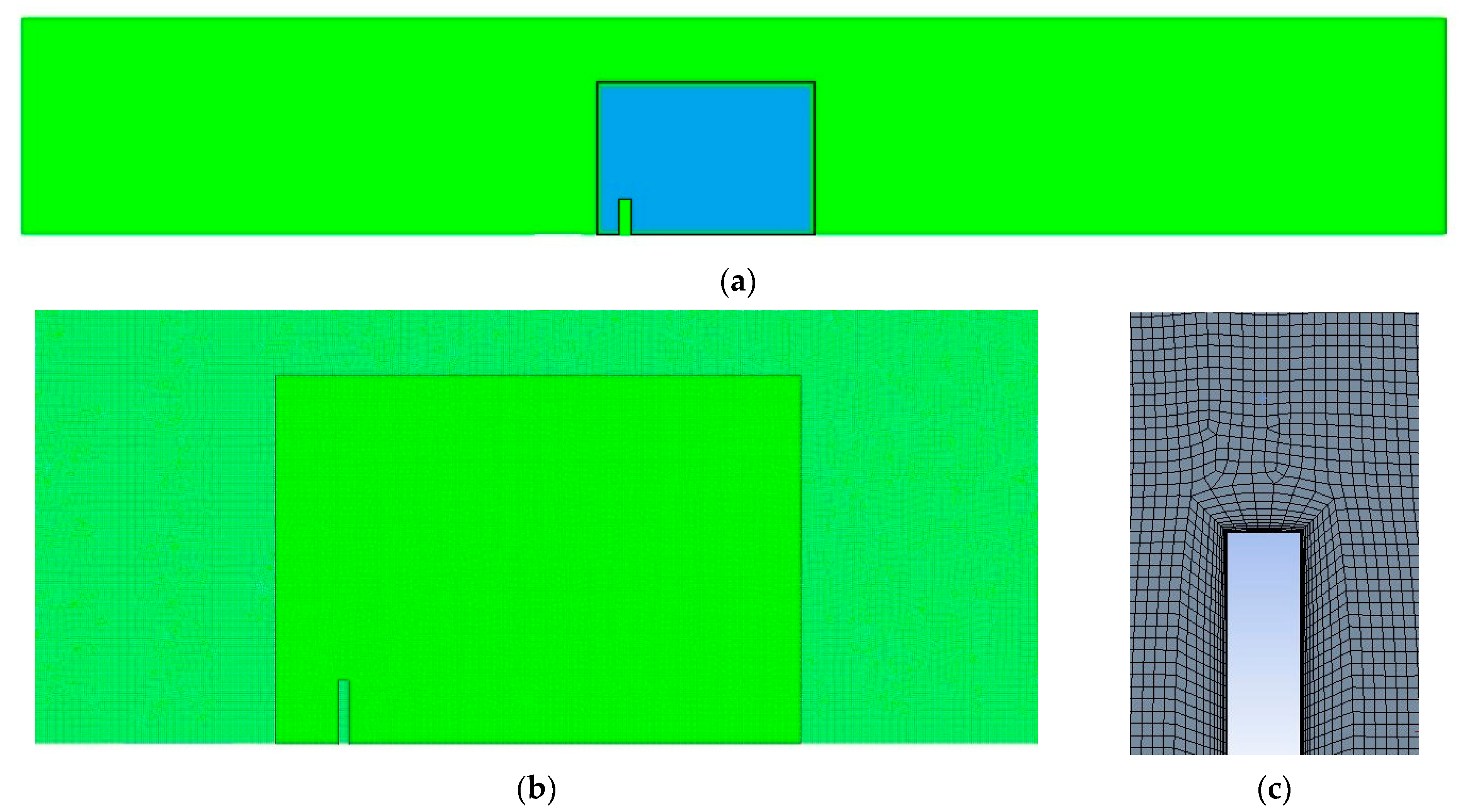
2.3. Simulation of the Dispersion Phenomena (the NR-CFD Model)
- The condition of horizontal homogeneity. The value of any property remains the same at any position with the same height.
- The inlet boundary condition should be known. At every vertical position at the inlet, the value of each variable should be a known input data.
- Agreement between the inlet and the ground boundary conditions. The condition of horizontal homogeneity requires that the ground boundary conditions for momentum and heat transfer agree with the inlet boundary conditions.
2.4. Use of Dimensionless Numbers to Study the Effect of Barrier Geometry on Pollutants Dispersion
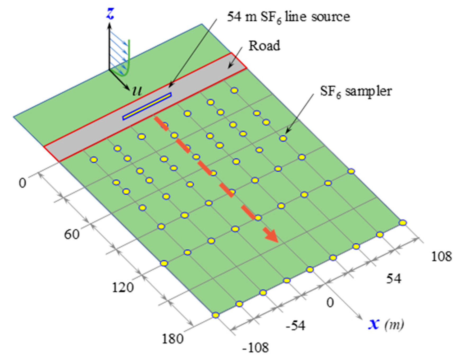
2.5. Validation with Experimental Results
2.6. Barrier Cost Evaluation
3. Results and Discussion
3.1. Comparison with Experimental Results
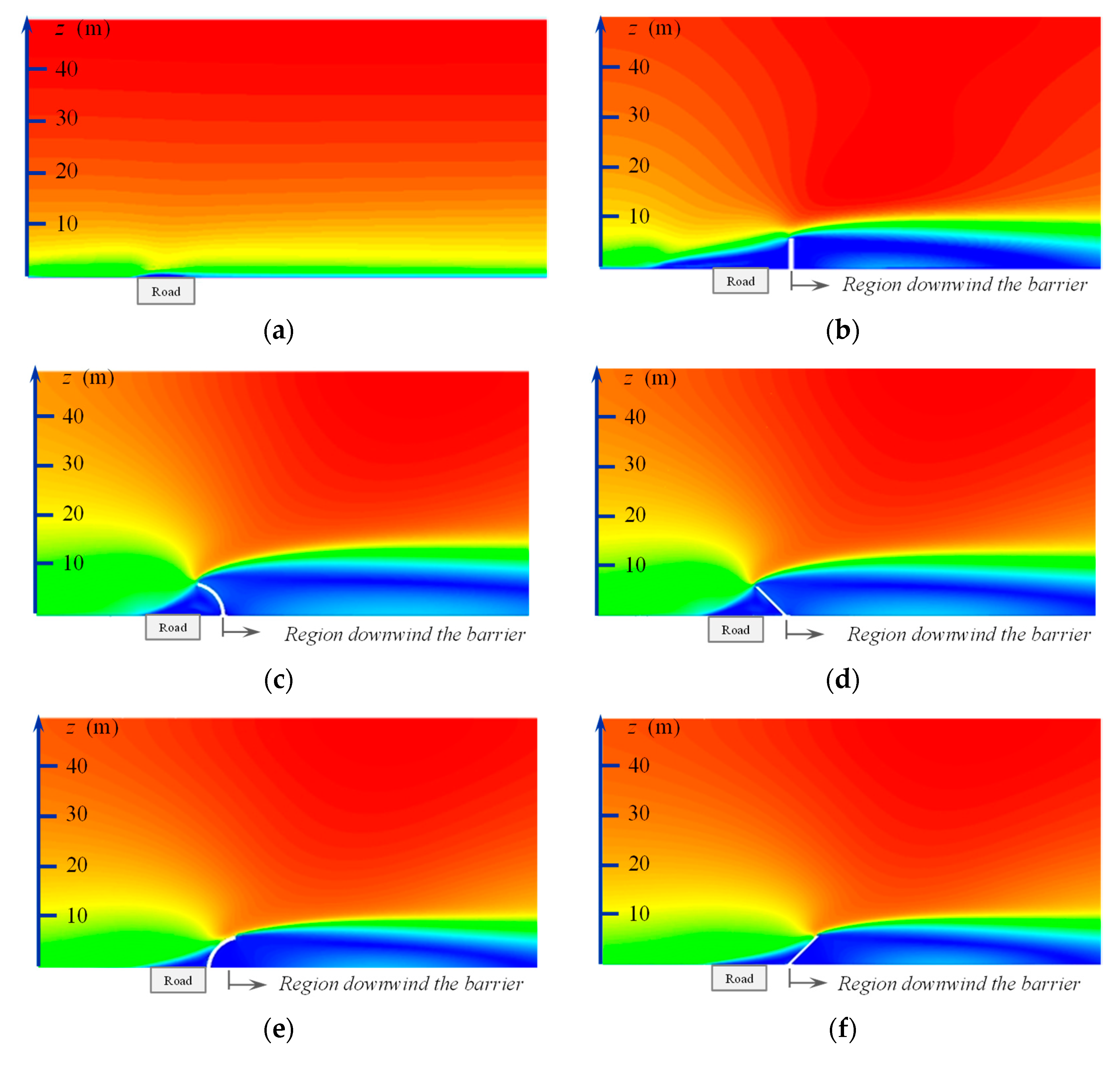
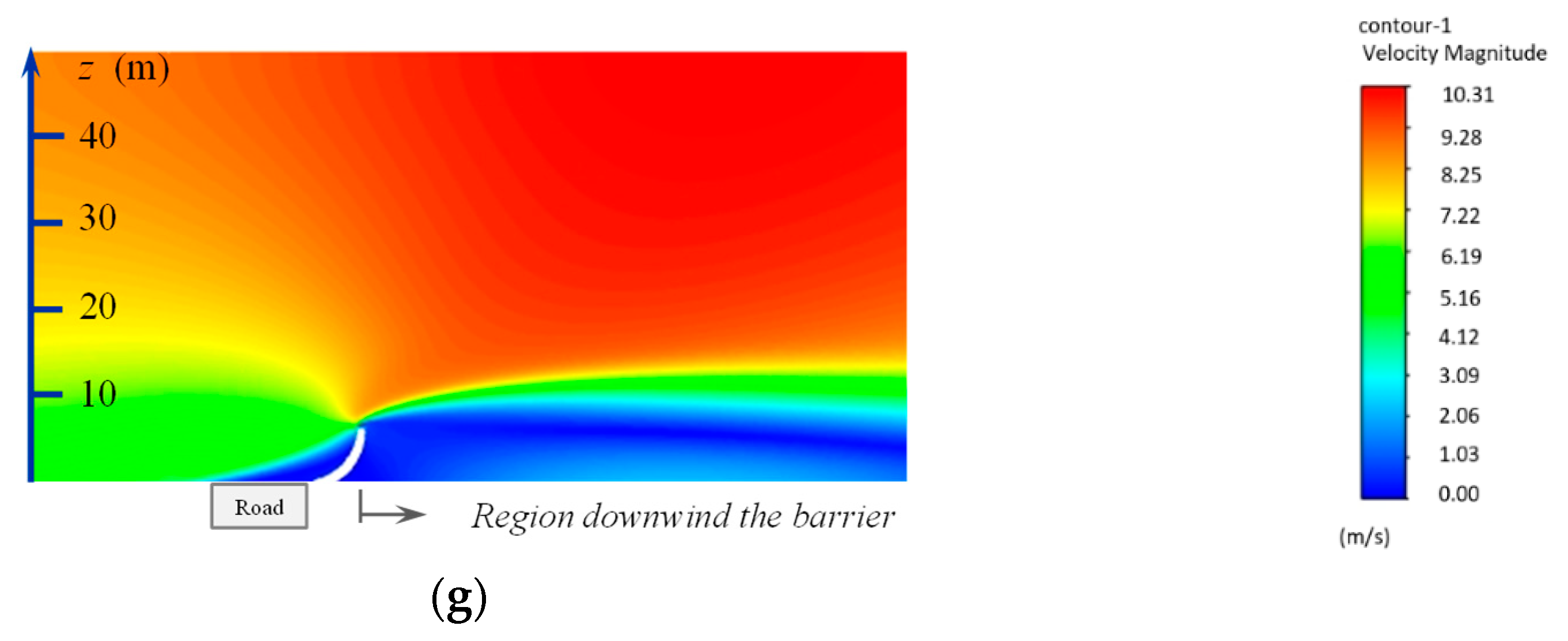
3.2. Resulting Velocity Contours
3.3. Vertical Mass Flux Profiles
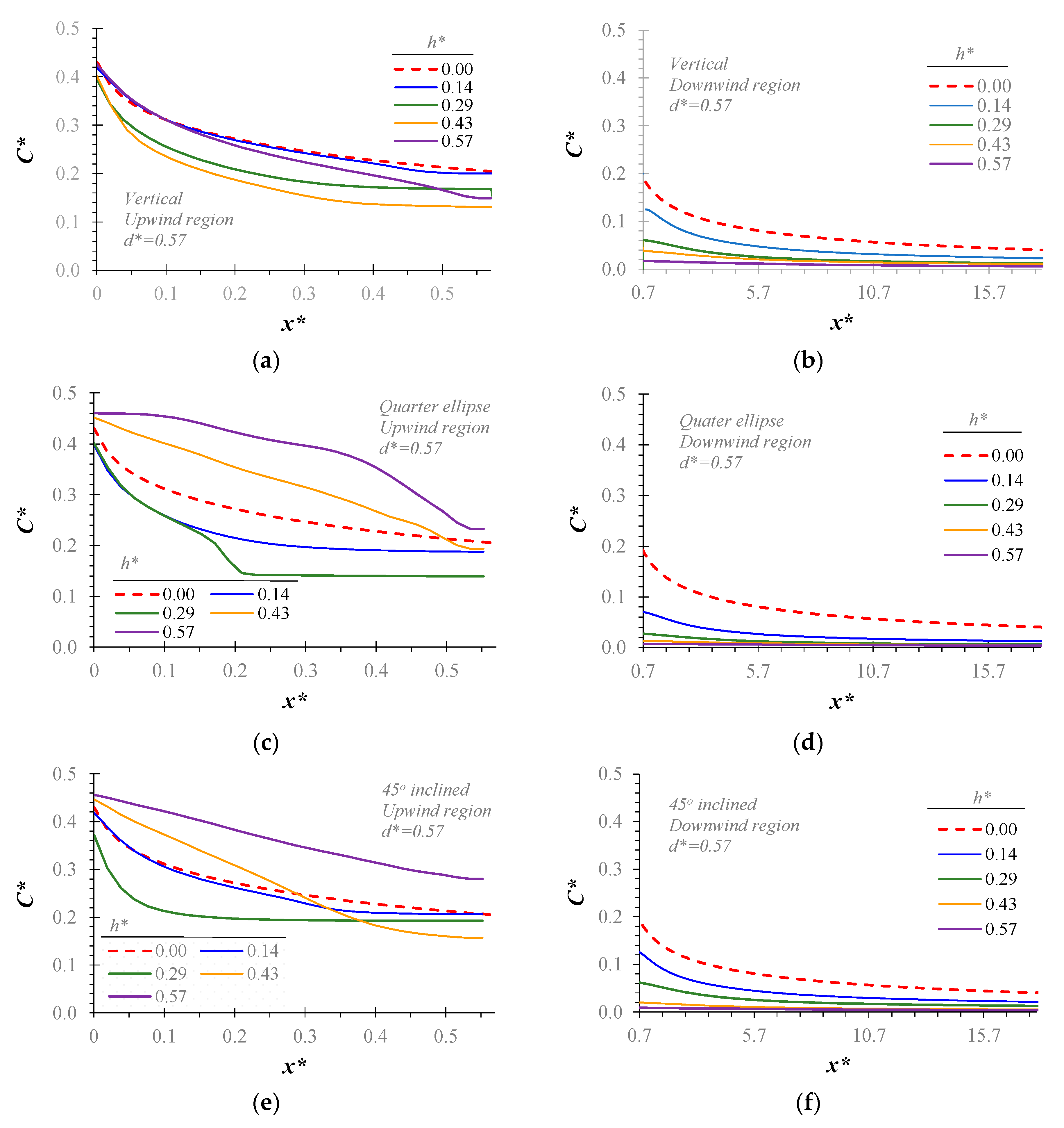
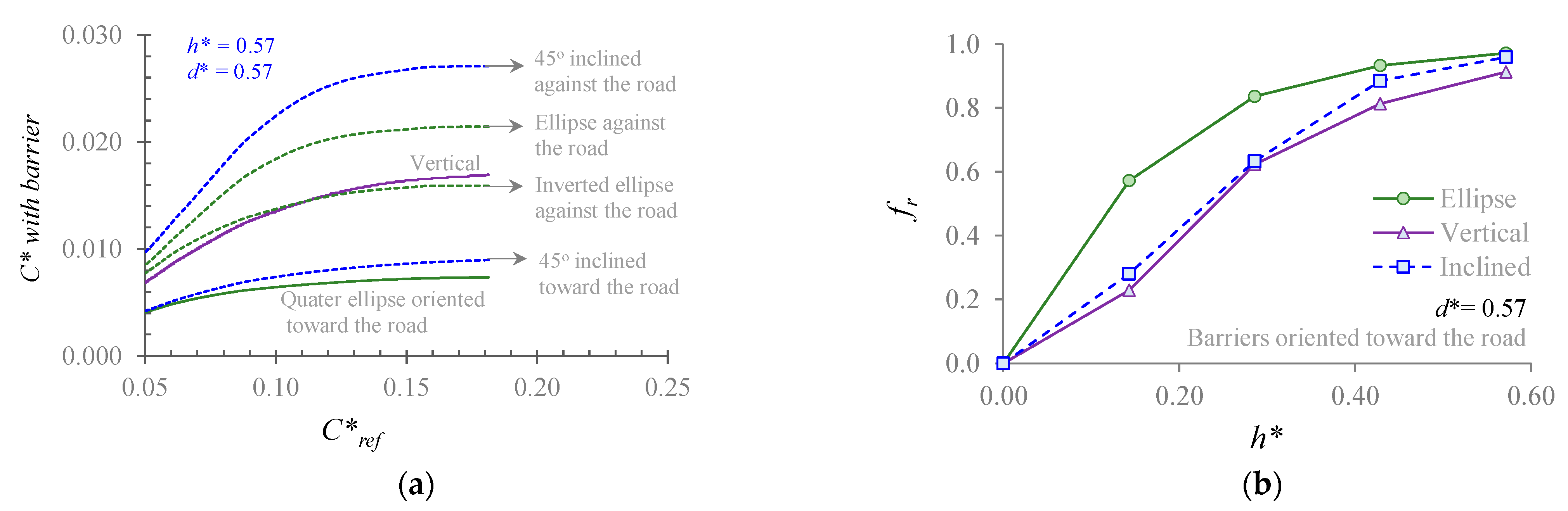
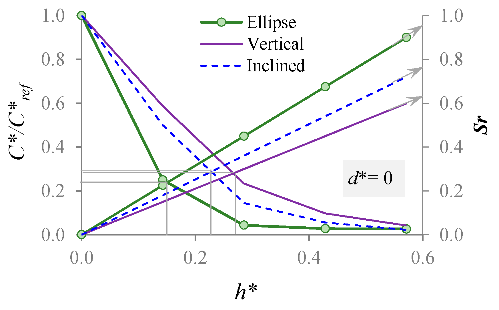
3.4. Effect of the Barrier Geometry and Size on Ground Pollutant Concentration
3.5. Effect of the Barrier Location on Ground Pollutant Concentration
3.6. Including Cost in the Selection of Barrier Size and Geometry
4. Conclusions
Author Contributions
Funding
Institutional Review Board Statement
Informed Consent Statement
Data Availability Statement
Acknowledgments
Conflicts of Interest
References
- Karner, A.A.; Eisinger, D.S.; Niemeier, D.A. Near-Roadway Air Quality: Synthesizing the Findings from Real-World Data. Environ. Sci. Technol. 2010, 44, 5334–5344. [Google Scholar] [CrossRef] [PubMed]
- Singh, S.; Adams, P.J.; Presto, A.A. Simulations of vehicle-induced mixing and near-road aerosol microphysics using computational fluid dynamics. AIMS Environ. Sci. 2018, 5, 315–339. [Google Scholar] [CrossRef]
- Nitta, H.; Sato, T.; Nakai, S.; Maeda, K.; Aoki, S.; Ono, M. Respiratory Health Associated with Exposure to Automobile Exhaust. I. Results of Cross-sectional Studies in 1979, 1982, and 1983. Arch. Environ. Health Int. J. 1993, 48, 53–58. [Google Scholar] [CrossRef] [PubMed]
- Riediker, M.; Cascio, W.E.; Griggs, T.R.; Herbst, M.C.; Bromberg, P.A.; Neas, L.; Williams, R.W.; Devlin, R.B. Particulate Matter Exposure in Cars Is Associated with Cardiovascular Effects in Healthy Young Men. Am. J. Respir. Crit. Care Med. 2004, 169, 934–940. [Google Scholar] [CrossRef] [PubMed]
- Finn, D.; Clawson, K.L.; Carter, R.G.; Rich, J.D.; Eckman, R.M.; Perry, S.G.; Isakov, V.; Heist, D.K. Tracer studies to characterize the effects of roadside noise barriers on near-road pollutant dispersion under varying atmospheric stability conditions☆. Atmospheric Environ. 2010, 44, 204–214. [Google Scholar] [CrossRef]
- Ning, Z.; Hudda, N.; Daher, N.; Kam, W.; Herner, J.; Kozawa, K.; Mara, S.; Sioutas, C. Impact of roadside noise barriers on particle size distributions and pollutants concentrations near freeways. Atmospheric Environ. 2010, 44, 3118–3127. [Google Scholar] [CrossRef]
- Clawson, K.L.; Eckman, R.M.; Johnson, R.C.; Carter, R.G.; Finn, D.; Rich, J.D.; Hukari, N.F.; Strong, T.; Beard, S.A.; Reese, B.R. Near Roadway Tracer Study; NOAA Technical Memorandum OAR ARL-260; Air Resources Laboratory: Idaho Falls, ID, USA, 2008. [Google Scholar]
- Heist, D.; Perry, S.; Brixey, L. A wind tunnel study of the effect of roadway configurations on the dispersion of traffic-related pollution. Atmospheric Environ. 2009, 43, 5101–5111. [Google Scholar] [CrossRef]
- Hagler, G.S.; Lin, M.-Y.; Khlystov, A.; Baldauf, R.W.; Isakov, V.; Faircloth, J.; Jackson, L.E. Field investigation of roadside vegetative and structural barrier impact on near-road ultrafine particle concentrations under a variety of wind conditions. Sci. Total. Environ. 2012, 419, 7–15. [Google Scholar] [CrossRef]
- Schulte, N.; Snyder, M.; Isakov, V.; Heist, D.; Venkatram, A. Effects of solid barriers on dispersion of roadway emissions. Atmospheric Environ. 2014, 97, 286–295. [Google Scholar] [CrossRef]
- Baldauf, R.W.; Isakov, V.; Deshmukh, P.; Venkatram, A.; Yang, B.; Zhang, K.M. Influence of solid noise barriers on near-road and on-road air quality. Atmospheric Environ. 2016, 129, 265–276. [Google Scholar] [CrossRef] [Green Version]
- Venkatram, A.; Heist, D.K.; Perry, S.G.; Brouwer, L. Dispersion at the edges of near road noise barriers. Atmospheric Pollut. Res. 2020. [Google Scholar] [CrossRef]
- Steffens, J.T.; Wang, Y.J.; Zhang, K.M. Exploration of effects of a vegetation barrier on particle size distributions in a near-road environment. Atmospheric Environ. 2012, 50, 120–128. [Google Scholar] [CrossRef]
- Steffens, J.T.; Heist, D.K.; Perry, S.G.; Zhang, K.M. Modeling the effects of a solid barrier on pollutant dispersion under various atmospheric stability conditions. Atmospheric Environ. 2013, 69, 76–85. [Google Scholar] [CrossRef]
- Adair, D.; Jaeger, M. Evaluation of model for air pollution in the vicinity of roadside solid barriers. Energy Environ. Eng. 2014, 2, 145–152. [Google Scholar]
- Jeong, S.J. A CFD Study of Roadside Barrier Impact on the Dispersion of Road Air Pollution. Asian J. Atmospheric Environ. 2015, 9, 22–30. [Google Scholar] [CrossRef]
- Morakinyo, T.E.; Lam, Y.F. Simulation study of dispersion and removal of particulate matter from traffic by road-side vegetation barrier. Environ. Sci. Pollut. Res. 2015, 23, 6709–6722. [Google Scholar] [CrossRef] [PubMed]
- Tong, Z.; Baldauf, R.W.; Isakov, V.; Deshmukh, P.; Zhang, K.M. Roadside vegetation barrier designs to mitigate near-road air pollution impacts. Sci. Total. Environ. 2016, 541, 920–927. [Google Scholar] [CrossRef]
- Ranasinghe, D.; Lee, E.S.; Zhu, Y.; Frausto-Vicencio, I.; Choi, W.; Sun, W.; Mara, S.; Seibt, U.; Paulson, S.E. Effectiveness of vegetation and sound wall-vegetation combination barriers on pollution dispersion from freeways under early morning conditions. Sci. Total. Environ. 2019, 658, 1549–1558. [Google Scholar] [CrossRef] [PubMed]
- Wang, S.; Wang, X. Modeling and analysis of highway emission dispersion due to noise barrier and automobile wake effects. Atmospheric Pollut. Res. 2021, 12, 67–75. [Google Scholar] [CrossRef]
- Reiminger, N.; Jurado, X.; Vazquez, J.; Wemmert, C.; Blond, N.; Dufresne, M.; Wertel, J. Effects of wind speed and atmospheric stability on the air pollution reduction rate induced by noise barriers. J. Wind. Eng. Ind. Aerodyn. 2020, 200, 104160. [Google Scholar] [CrossRef]
- Huertas, J.I.; Sánchez, D.F.P. An experimental and numerical study of air pollution near unpaved roads. Air Qual. Atmosphere Health 2019, 12, 471–489. [Google Scholar] [CrossRef]
- Huertas, J.I.; Martínez, D.S.; Prato, D.F. Effects of the atmospheric stability conditions on the dispersion of pollutants over flat areas. Scientific Rep. Nat. 2021. (Currently under review). [Google Scholar]
- Busini, V.; Rota, R. Influence of the shape of mitigation barriers on heavy gas dispersion. J. Loss Prev. Process. Ind. 2014, 29, 13–21. [Google Scholar] [CrossRef]
- Gerdroodbary, M.B.; Mokhtari, M.; Bishehsari, S.; Fallah, K. Mitigation of Ammonia Dispersion with Mesh Barrier under Various Atmospheric Stability Conditions. Asian J. Atmospheric Environ. 2016, 10, 125–136. [Google Scholar] [CrossRef] [Green Version]
- Franke, J.; Hellsten, A.; Schlünzen, H.; Carissimo, B. Best Practice Guideline for the CFD Simulation of Flows in the Urban Environment: COST Action 732 Quality Assurance and Improvement of Microscale Meteorological Models; Meteorological Institute: Hamburg, Germany, 2007. [Google Scholar]
- NZ Transport Agency. NZTA State Highway Noise; NZ Transport Agency: Wellington, New Zealand, 2010.
- U.S. Department of Transportation. Highway Traffic Noise: Analysis and Abatement Guidance; U.S. Department of Transportation: Washington, DC, USA, 2011.
- State of Queensland, Department of Transport and Main Roads. Transport Noise Management; State of Queensland, Department of Transport and Main Roads: Queensland, Australia, 2013.
- Arya, S. Introduction to Micrometeorology; Academic Press: Cambridge, MA, USA, 1988. [Google Scholar]
- Stull, R. The Atmospheric Boundary Layer. An Introduction to Boundary Layer Meteorology; Springer: Amsterdam, The Netherlands, 2005; pp. 375–418. [Google Scholar]
- Stull, R. Practical Meteorology: An Algebra-Based Survey of Atmospheric Science; University of British Columbia: Vancouver, BC, Canada, 2016; pp. 797–801. [Google Scholar]
- Blocken, B.B.; Gualtieri, C. Ten iterative steps for model development and evaluation applied to Computational Fluid Dynamics for Environmental Fluid Mechanics. Environ. Model. Softw. 2012, 33, 1–22. [Google Scholar] [CrossRef]
- Obukhov, A.M. Turbulence in an atmosphere with a non-uniform temperature. Boundary-Layer Meteorol. 1971, 2, 7–29. [Google Scholar] [CrossRef]
- Zoras, S.; Triantafyllou, A.; Deligiorgi, D. Atmospheric stability and PM10 concentrations at far distance from elevated point sources in complex terrain: Worst-case episode study. J. Environ. Manag. 2006, 80, 295–302. [Google Scholar] [CrossRef] [PubMed]
- Pieterse, J.; Harms, T. CFD investigation of the atmospheric boundary layer under different thermal stability conditions. J. Wind. Eng. Ind. Aerodyn. 2013, 121, 82–97. [Google Scholar] [CrossRef] [Green Version]
- Xia, Q.; Niu, J.; Liu, X. Dispersion of air pollutants around buildings: A review of past studies and their methodolo-gies. Indoor Built Environ. 2014, 23, 201–224. [Google Scholar] [CrossRef]
- Alinot, C.; Masson, C. k-ϵ Model for the Atmospheric Boundary Layer Under Various Thermal Stratifications. J. Sol. Energy Eng. 2005, 127, 438–443. [Google Scholar] [CrossRef]
- Wang, Y.J.; Zhang, K.M. Modeling Near-Road Air Quality Using a Computational Fluid Dynamics Model, CFD-VIT-RIT. Environ. Sci. Technol. 2009, 43, 7778–7783. [Google Scholar] [CrossRef] [PubMed]
- ANSYS. Theory Guide; ANSYS, Inc.: Canonsburg, PA, USA, 2012. [Google Scholar]
- Walvoord, M.A.; Andraski, B.J.; Green, C.T.; Stonestrom, D.A.; Striegl, R.G. Field-Scale Sulfur Hexafluoride Tracer Experiment to Understand Long Distance Gas Transport in the Deep Unsaturated Zone. Vadose Zone J. 2014, 13, 1–10. [Google Scholar] [CrossRef] [Green Version]
- Blocken, B.; Stathopoulos, T.; Carmeliet, J. CFD simulation of the atmospheric boundary layer: Wall function problems. Atmospheric Environ. 2007, 41, 238–252. [Google Scholar] [CrossRef]
- ANSYS. User Guide; ANSYS, Inc.: Canonsburg, PA, USA, 2012. [Google Scholar]
- Rüedi, I. WMO Guide to Meteorological Instruments and Methods of Observation: WMO-8 Part I: Measurement of Meteorological Variables, Chapter 1; World Meteorological Organization: Geneva, Switzerland, 2006. [Google Scholar]


| Author(s) | Description | Year | CFD | Experimental Measurements | Geometry Variation | Cost Evaluation |
|---|---|---|---|---|---|---|
| Finn et al. | Tracer gas dispersion study with a straight noise barrier near roadway | 2009 | x | ✓ | x | x |
| Ning et al. | Impact of noise barriers on particle pollutants size distributions and concentrations near freeways | 2010 | x | ✓ | x | x |
| Hagler et al. | Use of tree stands and brick noise barriers for mitigation of roadside ultrafine particles | 2012 | x | ✓ | ✓ | x |
| Steffens et al. | Vegetation barrier model to mitigate roadside pollutant dispersion in terms of LAD | 2012 | ✓ | ✓ | x | x |
| Steffens et al. | Simulation of tracer gas dispersion under twelve different roadway configurations | 2013 | ✓ | ✓ | ✓ | x |
| Adair and Jaeger | Evaluation of solid barriers performance for the mitigation of air pollution with NOx | 2014 | ✓ | ✓ | ✓ | x |
| Busini et al. | Barrier shape effect on LNG dispersion due to pipe leaks | 2014 | ✓ | ✓ | ✓ 1 | x |
| Schulte et al. | Semiempirical dispersion model of roadside barriers | 2014 | x | ✓ | ✓ | x |
| Jin Jeong | Roadside barrier impact on the dispersion of road air CO for several road configurations | 2015 | ✓ | ✓ | x | x |
| Morakinyo and Lam | PM dispersion and removal via natural barrier use | 2015 | ✓ | ✓ | ✓ | x |
| Baldauf et al. | Noise barriers for the mitigation of on-road and downwind pollutants (NOx, UFP) | 2016 | x | ✓ | x | x |
| Tong et al. | Effects of vegetative and solid barriers on the mitigation of particle matter pollutants | 2016 | ✓ | ✓ | ✓ | x |
| Gerdroodbary et al. | Mesh barrier use to mitigate ammonia dispersion near pipelines | 2016 | ✓ | ✓ | ✓ 2 | x |
| Ranasinghe et al. | Vegetation and barrier combination effect on pollutant dispersion near roads | 2019 | x | ✓ | x | x |
| Wang and Wang | Effect of vehicle shape and barrier use on highway emission dispersion | 2020 | ✓ | ✓ | x | x |
| Reiminger et al. | Effect of wind speed and atmospheric stability on pollutant reduction rate due to barrier use | 2020 | ✓ | ✓ | x | x |
| Venkatram et al. | Pollutant dispersion near road-side barrier edges | 2021 | x | ✓ | x | x |
Publisher’s Note: MDPI stays neutral with regard to jurisdictional claims in published maps and institutional affiliations. |
© 2021 by the authors. Licensee MDPI, Basel, Switzerland. This article is an open access article distributed under the terms and conditions of the Creative Commons Attribution (CC BY) license (http://creativecommons.org/licenses/by/4.0/).
Share and Cite
Huertas, J.I.; Aguirre, J.E.; Lopez Mejia, O.D.; Lopez, C.H. Design of Road-Side Barriers to Mitigate Air Pollution near Roads. Appl. Sci. 2021, 11, 2391. https://doi.org/10.3390/app11052391
Huertas JI, Aguirre JE, Lopez Mejia OD, Lopez CH. Design of Road-Side Barriers to Mitigate Air Pollution near Roads. Applied Sciences. 2021; 11(5):2391. https://doi.org/10.3390/app11052391
Chicago/Turabian StyleHuertas, Jose I., Javier E. Aguirre, Omar D. Lopez Mejia, and Cristian H. Lopez. 2021. "Design of Road-Side Barriers to Mitigate Air Pollution near Roads" Applied Sciences 11, no. 5: 2391. https://doi.org/10.3390/app11052391