Article

Experiments with Neural Networks in the Identification and Control of a Magnetic Levitation System Using a Low-Cost Platform

by
Bruno E. Silva
1 and
Ramiro S. Barbosa
2,*
1
Department of Electrical Engineering, Institute of Engineering—Polytechnic of Porto (ISEP/IPP), Rua Dr. António Bernardino de Almeida, 431, 4249-015 Porto, Portugal
2
Research Group on Intelligent Engineering and Computing for Advanced Innovation and Development (GECAD), Instituto Superior de Engenharia do Porto (ISEP), Rue Dr. António Bernardino de Almeida 431, 4200-072 Porto, Portugal
*
Author to whom correspondence should be addressed.
Appl. Sci. 2021, 11(6), 2535; https://doi.org/10.3390/app11062535
Submission received: 23 January 2021 / Revised: 26 February 2021 / Accepted: 8 March 2021 / Published: 12 March 2021
(This article belongs to the Section Computing and Artificial Intelligence)

Abstract

:
In this article, we designed and implemented neural controllers to control a nonlinear and unstable magnetic levitation system composed of an electromagnet and a magnetic disk. The objective was to evaluate the implementation and performance of neural control algorithms in a low-cost hardware. In a first phase, we designed two classical controllers with the objective to provide the training data for the neural controllers. After, we identified several neural models of the levitation system using Nonlinear AutoRegressive eXogenous (NARX)-type neural networks that were used to emulate the forward dynamics of the system. Finally, we designed and implemented three neural control structures: the inverse controller, the internal model controller, and the model reference controller for the control of the levitation system. The neural controllers were tested on a low-cost Arduino control platform through MATLAB/Simulink. The experimental results proved the good performance of the neural controllers.

1. Introduction

From a very early age, control has played a fundamental role in society, being currently present in most systems with several control techniques. Among the most used algorithms, the Proportional-Integral-Derivative (PID) controller stands out, which is part of the classic control methods [1,2]. However, with scientific and technological developments in the field of Artificial Intelligence (AI), there are now control techniques called intelligent control, which include methods such as fuzzy control, evolutionary control, and neural control [3,4,5,6]. Neural networks are now widely studied and used in the areas of image processing [7,8], complex optimization problems [9], systems control [10], among others.
By applying AI techniques like neural networks to a control system, the algorithms obtained are capable of solving problems that classical control cannot, due to the universal approximation capabilities of the neural networks. In control systems, the objective is to find an appropriate feedback function that maps the measured outputs in order to control the inputs. For that, there are several architectures that use neural networks that can be employed [11,12]. This type of control can be applied to several types of systems; however, its performance stands out compared to other techniques in the control of nonlinear and unstable systems [13,14].
Magnetic levitation consists of the suspension of an object in the air, using magnetic forces of attraction or repulsion, thus counteracting the gravitational force applied to that object [15,16]. Nowadays, it is increasingly used in areas of passenger and cargo transportation because it drastically reduces the mechanical losses that conventional systems entail [17]. However, systems that employ magnetic levitation often require a robust control algorithm as they are normally unstable and nonlinear [18,19]. Magnetic suspension controlling a DC electromagnet is the most used method, from advanced land transport to contactless bearings for high and low speeds. This is a method that has been studied for over a century, but which is constantly improving due to technological advances in several areas such as power electronics, control theory, and mechanics [15,17].
A similar magnetic levitation system is studied in [11], where the authors use a Nonlinear Autoregressive Moving Average (NARMA) neural network to perform the system identification and a neural network that learns the system dynamics, thus emulating its response to the desired input. The authors then use a neural network predictive controller to control the levitation system. Studies on the same system are conducted in [20], where a model reference controller is trained to control the system. In Reference [21], the authors propose an RBF ARX model based MPC strategy for the ball position control of a fast-response magnetic levitation system. The applied strategy worked like a time-varying locally linear ARX model-based linear MPC process. It was illustrated that the RBF-ARX-MPC is effective and feasible in modeling and controlling the fast-responding, strongly nonlinear, and open-loop unstable system. Work [22] presents an application of magnetic levitation to stabilization and tracking control of a single degree-of-freedom mass-spring–damper vibrating mechanical system. An output feedback control scheme based on differential flatness for global stabilization and asymptotic tracking tasks of some desired reference position trajectory is proposed. Experimental and simulation results showed the efficient and satisfactory performance of the tracking control scheme and the acceptable signal estimation. Other similar mechanisms such as air levitation systems are also considered in various works. In Reference [23], the control of an air levitation system with limited sensing is studied. It uses a sliding mode control, but it was modified to take only a measure of the position, which is the only one available. The experimental results show the feasibility of the controller and assess its performance in a real system. In Reference [24], a low-cost air levitation system to be used in both a virtual and a remote version is proposed. It provides a complete open-source and open-hardware remote lab solution that is low-cost and easy to replicate.
This work applies several neural control schemes to a challenging system like the nonlinear and unstable magnetic levitation system to test the performance of neural controllers in a low-cost hardware. Nowadays this type of hardware is extensively used both in academia and scientific projects and its validation to incorporate more recent technologies such as neural networks is needed. The main differentiation of this contribution with respect to former control methods is that the system in many of those research works used repulsion to oppose the gravitational acceleration and the suspended magnet was constrained so that it could only move in the vertical direction. In this article, the system uses attraction to counteract gravity and the suspended magnet is not constrained in any way, so it is more susceptible to perturbations. Moreover, in this work, we apply several neural control structures and compare the results among them to verify the feasibility of each control structure in the control of the levitation system. Also, some linear classical controllers are developed to give the training data for the neural controllers, as well to enhance the better performance of the neural controllers. In fact, the neural controllers can control the levitation system in a wider-range of operation in contrast with the linear controllers, which only operates on small variations around the linearized point. Furthermore, the proposed neural controllers are implemented in a low-cost hardware, which can be easily built and used for in site laboratory experiments or take-home laboratories.
Here, we describe the whole process of implementing a neural controller applied to a magnetic levitation system, as well as some classical controllers for the comparison of the results. Section 2 shows the details of the hardware setup, whereas Section 3 presents the modeling and identification of the levitation system. In Section 4 described the design of the two classical controllers with the objective of providing the training data for the neural controllers. Section 5 describes the implementation and testing of three neural controllers on a real levitation system. Finally, Section 6 draws the main conclusions and addresses perspectives to future developments of the presented work.

2. System Architecture

In this system, a microcontroller sends a Pulse Width Modulation (PWM) signal to a driver circuit that converts it into a suitable signal to control the electromagnetic circuit. The position of the magnet and the current flowing in the electromagnet are obtained by using the 10 bit Analog-to-Digital Converter (ADC) of the microcontroller ATmega2560 to convert the signals sent by the sensors. The position and current sensors are linear Hall effect sensors, respectively the A1324 and ACS711 of Allegro Microsystems [25,26]. The system is monitored via an USB serial connection through microcontroller using Simulink together with the Simulink Support Package for Arduino Hardware Add-on [27]. Figure 1 illustrates the block diagram of the general system architecture.
The driver circuit is represented in Figure 2, and it contains the diode (D) for the currents generated by the inverse polarities due to the inductive nature of the system, a pull-down resistor (R p d = 4.7 k Ω ) to prevent the gate of the Metal–Oxide–Semiconductor Field-Effect Transistor (MOSFET) (Q) from floating, and a capacitor (C = 1.0 mF) to ensure that the 5 V supplied by the voltage regulator is stable. It is a simple driver that effectively supplies the electromagnetic system with the current required to levitate the magnetic disc.
In Figure 2 the orange rectangle represents the electromagnet, where R e and L e are the electromagnet resistance and inductance, respectively. As shown in the Figure 3, the magnetic disc stays below the electromagnet and the position sensor stays directly under the electromagnet and as such it will suffer the influence of the magnetic field of both the magnetic disc and the electromagnet.
The parameters values of the system are listed on Table 1, where the weight, diameter, and thickness correspond to the disc.
A photo of the experimental levitation system is presented in Figure 4. A passive heat-sink was used so the voltage regulator was able to supply the current needed to the electromagnet.
This system used a Funduino Mega 2560 board, which is a copy of Arduino Mega 2560. The board has 8 bits ATmega2560 microcontroller from Microchip. This microcontroller was chosen due to the available Flash Memory and Static Random-Access Memory (SRAM), as shown in the specifications of Table 2. This is one of the most expensive parts of the control system, costing about 10 euros. With the Simulink Add-on, the code will be generated by Simulink model and deployed on the microcontroller. The sampling period for the controllers was set to T = 0.003 s, which was the maximum value found for obtaining a steady stable levitation using the root-locus method described in Section 4 for the design of the classical linear controllers. The same sampling interval was adopted in the design of the neural controllers of Section 5.

3. System Analysis

The magnetic field is generated by the electromagnet in order to levitate the neodymium disc, as shown in Figure 5. The system is controlled through the voltage supplied to the electrical system terminals, which in turn generates the current that produces the magnetic field. As shown in the figure, v ( t ) is the applied voltage, i ( t ) the generated current, e z ( t ) , and e i ( t ) the voltages at the terminals of the position and current sensors, respectively, z ( t ) the distance from the magnetic disk to the sensor, F m the magnetic force generated by the magnetic field of the electromagnet, and F g the force caused by gravity.

3.1. Electromagnetic System Modeling

The equation that describes the resultant force on the neodymium disc is given by [28,30]:
m d 2 z ( t ) d t 2 = m g k i ( t ) z ( t ) 4 ,
where m is the mass of the levitating object, g is the acceleration due to gravity, and k is a magnetic constant related to turn ratio and cross sectional area of the electromagnet. As shown, it is the sum of the gravitational pull on the disc and the magnetic force. The force applied by the magnetic field generated by the electromagnet on the disc is influenced by the current that is generating the magnetic field, and the distance of the disc to the electromagnet [28,30].
The equation of the electromagnet circuit is:
v ( t ) = R e i ( t ) + L e d i ( t ) d t ,
where R e and L e are the resistance and inductance of the electromagnet, respectively.
In order to obtain a stable levitation of the neodymium disc, the magnetic force of attraction needs to be equal to the gravitational pull so that the resultant force in the disc is null. So in the equilibrium point the system obeys the following conditions:
d 2 z ( t ) d t 2 = 0 ,
z ( t ) = z e q ,
i ( t ) = i e q .
Therefore, in the equilibrium point, the magnetic constant is given by:
k = m g z e q 4 i e q .
As can be seen, the above equations represent a nonlinear system, and to design a linear controller the system must be linearized around an equilibrium point [31], ( i e q , z e q , v e q ) , in which Δ i ( t ) , Δ z ( t ) , and Δ v ( t ) denote small variations around it, such as:
i ( t ) = i e q + Δ i ( t ) ,
z ( t ) = z e q + Δ z ( t ) ,
v ( t ) = v e q + Δ v ( t ) .
Applying the Taylor series expansion in (1) and (2) around ( i e q , z e q , v e q ) , we obtain the linearized equations:
m d 2 Δ z ( t ) d t 2 = m g k i e q z e q 4 + k 4 i e q z e q 5 Δ z ( t ) k 1 z e q 4 Δ i ( t ) ,
Δ v ( t ) = R Δ i ( t ) + L d Δ i ( t ) d t .
Replacing (6) into (10), we get:
d 2 Δ z ( t ) d t 2 = 4 g z e q Δ z ( t ) g i e q Δ i ( t ) .
With Equations (11) and (12) linearized, the Laplace transform is used to obtain the transfer function between the supplied voltage and the distance of the disc from the electromagnet, as:
Δ Z ( s ) Δ V ( s ) = g i e q ( L s + R ) ( s 2 4 g z e q ) .
Note that (13) is an unstable system since one of the poles is in the right-half of the s-plane.

3.2. Sensors Parameterization

The Hall effect sensors produce a voltage related to the magnetic field they are inserted in. The voltages generated by both sensors have a portion related to the quiescent voltage they produce [25,26], the influence of the current and, in the case of the position sensor, a portion related to the distance of the magnetic disc.
The equations of the output voltages for the current and position Hall-effect sensors are of the form, respectively:
e i ( t ) = m f ( i ( t ) ) + b ,
e z ( t ) = α + β g ( z ( t ) ) + γ f ( i ( t ) ) ,
where m, b, α , β , e, γ are the constants to be determined.
To obtain the sensors constants, first, the quiescent voltages of the current and position sensors were measured as b = 2.5220 and α = 2.4829 V, respectively. After the current and distance were increased in small steps in order to observe the variation of the respective output voltages, as shown in Figure 6 and Figure 7. In both figures, the value of the quiescent voltages were removed, so that it facilitates the determination of the constants through regression.
With the voltage data points of Figure 6 and Figure 7 we used the Trendline option of Microsoft Excel to obtain the linear Equations (16) and (17), which translates the influence of the current on both current and position sensors, respectively:
e i i ( t ) = m f ( i ( t ) ) = 0.1447 i ( t ) ,
e z i ( t ) = γ f ( i ( t ) ) = 0.3339 i ( t ) ,
where m = 0.1447 and γ = 0.3339 V/A. The expression for the influence of the distance on the position sensor was obtained as:
e z z ( t ) = β g ( z ( t ) ) = 4.4941 × 10 6 1 z ( t ) 3 ,
where β = 4.4941 × 10 6 Vm 3 . In this case the current sensor does not suffer any influence by the movement of the disc. All regressions obtained a good R 2 , 0.9988 for e i i , 0.9995 for e z i , and 0.9961 for e z z .
Replacing the determined parameter values in (14) and (15), we arrive to the following equations for the output voltage of each sensor:
e i ( t ) = 0.1447 i ( t ) + 2.5220 ,
e z ( t ) = 2.4829 + 4.4941 × 10 6 1 z ( t ) 3 + 0.3339 i ( t ) ,
Because this system uses the 10 bits ADC of the ATMega2560, Equations (19) and (20) are converted to Analog-to-Digital Units (ADU), where 5 V corresponds to 1023 ADU, yielding:
A D C i ( t ) = 29.569 i ( t ) + 516 ,
A D C z ( t ) = 508 + 1090 1 z ( t ) 3 + 68.274 i ( t ) ,
where in order to facilitate the calculation, the distance was also converted from m to cm, and as such β is now 1090 ADUcm3.
Table 3 lists the converted constants corresponding to both sensors.
With the sensor constants determined, we used the Solver tool from Microsoft Excel to optimize the constants. To obtain the Table 4, we placed the magnetic disc at different distances and applied enough voltage to the electromagnet to pull the disc up.
The values of the ADC i and ADC z were measured at when the magnetic disc started to rise. Then, we calculated the current (i c a l c ) corresponding to ADC i using Equation (21), and with those values, we calculated the distance (z c a l c ) from Equation (22). Then we calculated the sum of the absolute difference between the real distance of the disc (z) and z c a l c . The Solver tool was then used to change the sensor constants in order to minimize that sum. Table 4 shows the calculated distances after optimizing the values of the constants (z o p t i m ).
Table 5 shows the optimized parameter values corresponding to both sensors.
Rearranging (21) and (22) and substituting the values in Table 5, we obtain the expressions for the computation of the current i ( t ) and distance z ( t ) :
i ( t ) = 0.03324 A D C i ( t ) 17.1632 ,
z ( t ) = 1123.801 A D C z ( t ) 507.045 69.474 i ( t ) 3 .
Lastly, some tests were performed to determine the equilibrium point, as the current for which the magnetic disc is almost lifted off at 2 cm from the electromagnet. The measured value was 0.27 A, and thus ( i e q , z e q ) = ( 0.27 A , 2 cm ) . Substituting the system parameters in (13), the resulting transfer function is:
G ( s ) = 2.4222 × 10 5 ( s + 200 ) ( s + 44.29 ) ( s 44.29 ) .

4. Classical Controllers

Due to the inherent instability of the system, it is not possible to apply a random signal directly to the system in order to get the training data. So linear controllers were designed and tested in order to obtain the training data for the neural networks.
In order to simplify the design of the controllers, we used the dominant pole approximation [32,33], that states that the closer poles to the imaginary axis are considered the dominant poles because the transient response of the system is characterized by them. In this particular system, because the ratio between the furthest pole from the imaginary axis ( s = 200 ) and the dominant pole ( s = 44.29 ) is at least four, the transfer function (25) can be rewritten, while maintaining the static gain of the system, as:
G d p ( s ) = 1211.1 ( s + 44.29 ) ( s 44.29 ) .
Using a zero-order-hold (ZOH) with a sampling period of T = 0.003 s, the discrete system has the following transfer function:
G p d ( z ) = 5.458 × 10 2 ( z + 1 ) ( z 1.142 ) ( z 0.8756 ) .
The first controller was a lead compensator in order to improve the stability of the closed-loop system [32,33]. The root-locus method [32] is applied for a time response with less than 5% overshoot and a rise time of ten times the sampling period ( t r = 0.03 s), yielding:
D l e a d ( z ) = 6.8316 z 0.8756 z 0.6806 .
From the lead compensator we designed a lead–lag compensator to reduce the steady state error [32,33]. The root-locus method was again used, and in order to maintain the stability of the transient response provided by the lead compensator, we design the lag portion of the controller with a zero and pole extremely near z = 1 [34]. The zero obtained for the lag portion was z = 0.9979 and for the pole z = 1 , thus providing an integrative action to the lead–lag controller:
D l e a d l a g ( z ) = 6.823 z 2 + 12.8 z 5.969 z 2 1.68 z + 0.6804 .
The simulated system response is depicted in Figure 8. We observe that both controllers have the same transient response but the integrative action of the lead–lag compensator eliminates the steady-state error.
Figure 9 shows the real-time Simulink diagram used to test the classical controllers. A similar control diagram will be used for the neural controllers.
In Figure 10 we present the experimental responses of the system to a step input for the lead and lead–lag compensators. As shown, both controllers can maintain a stable levitation; however the lead–lag compensator generates an output response around the desired step reference, and thus having an improved steady-state error.

5. Neural Control Strategies

In order to obtain a good performance of neural networks, a good training data set is required. With the designed classical controllers, an appropriate reference signal can be developed and applied to the system. The lead–lag compensator was the chosen controller as it provides the best response, as demonstrated in the previous section.
The reference signal is a random signal with varying amplitudes at different frequencies in order to get the most rich data possible of the system within the limits of the classical lead–lag controller. Figure 11 shows the reference signal and the system response, whereas Figure 12 presents the corresponding control signal.

5.1. System Identification

The system identification was done by using Nonlinear AutoRegressive eXogenous (NARX) neural networks of type [12]:
y n n ( n + 1 ) = f [ u ( n ) , u ( n 1 ) , , u ( n i ) , y ( n ) , y ( n 1 ) , , y ( n i ) ] ,
where u ( n ) is the input control signal and y ( n ) the output system response.
Several two-layer feed-forward networks with hyperbolic tangent hidden neurons and one linear output neuron were trained. Figure 13 shows one example of a neural network using 10 past values of input and output signals and 15 neurons on the first layer, denoted as 10d15n. We use the Levenberg–Marquardt Backpropagation algorithm to minimize the Mean Squared Error (MSE) between the output of the network and system response [20]. Table 6 shows the MSE obtained for each network after training.
After some trials, the neural network that provided the best MSE is composed of 10 neurons on the first layer and using 10 past values of the input and output signals (10d10n). Table 7 lists the MSE of the best performing networks for the step, sinusoidal, and sawtooth reference signals. The Total column represents the sum of the other three columns, where we confirm that the 10d10n network has the best general performance.
In Figure 14, we illustrate the responses of the system with the 10d10n identification network when controlled with the lead–lag compensator, for the step, sinusoidal, and sawtooth reference signals. A time slot of only 5 s is used for the step response to provide a clear view of the transient behavior of the system; the other input references required more time to see multiple periods of the signals. We verify that the network follows the system response very well without having learned the noise and perturbations of the system.
Note that this identification network will be used as a neural model of the levitation system in the simulation of the neural control systems reported in next subsections.

5.2. Inverse Neural Controller

An inverse model controller learns the inverse dynamics of the system, receiving as inputs the reference signal r ( n ) , past samples of the control signal u ( n ) , and system output y ( n ) , of the form:
u ( n ) = f [ r ( n ) , y ( n ) , , y ( n i ) , u ( n 1 ) , , u ( n 1 i ) ] .
The block diagram of Figure 15 shows the configuration of an inverse model controller, where the controller receives as inputs the reference r ( n ) , the system output y ( n ) , and past value of control signal u ( n 1 ) . In order to obtain a more robust controller with a better performance we can use more past values of output and control signals.
In a first attempt, two-layer networks were created and trained, but their performance was poor. Thus, we trained two hidden layer networks, the first with one hyperbolic tangent neuron and the second with sigmoid neurons followed by one Rectified Linear Unit (ReLU) output neuron. The ReLU function in the last layer is used because the controller can not provided a negative value to the system. The Levenberg–Marquardt back-propagation was again used to train the networks, and the training data were pre-processed to the interval [0,1].
After training and testing different networks, we list in Table 8 the MSE of the best performing networks for the step, sinusoidal, and sawtooth reference signals.
The chosen network was the one with best performance—1th5s5d network, which means one neuron on first layer (1th), five neurons on the second layer (5s), and five past values of control and system output (5d). Figure 16 illustrates this network, where the input consists of 11 sample values corresponding to 5 past values of control and system output, and the reference value. The bigger networks with more neurons and more past values did not achieve the same performance because they started to overfit and lose their generalization capabilities.
Figure 17 depicts the experimental responses of the system controlled by the 1th5s5d inverse neural network, where the reference signal is represented in blue and the system response in red.
We verify that the inverse model network can stabilize the system, however it presents a steady-state error in all reference signals.
In order to improve further the system response, we can insert an adaptive block whose output is added to the output of the inverse model network, defined by expression:
B = β i = 0 k ( r ( i ) z ( i ) ) ,
where β is an adjustable gain between 0 and 1 [35]. Note that because the system has a negative gain, the tuning parameter β has also a negative gain. It is expected that the addition of this scheme will eliminate the steady-state error.
When implementing the adaptive block and testing the system, we obtained the responses in Figure 18. It is clear that the steady-state error that the inverse model network entails was eliminated with the addition of the adaptive block.
For comparison of the controllers we compute the performance indexes of the Integral Square Error (ISE), the Integral Absolute Error (IAE), and the Integral Time Absolute Error (ITAE), as:
I S E = 0 T s i m e 2 ( t ) d t ,
I A E = 0 T s i m | e ( t ) | d t ,
I T A E = 0 T s i m t | e ( t ) | d t .
where e ( t ) is the error between the reference signal and the actual position response of the levitation system. We use T s i m = 40 s that proved to be enough in order to compare the responses of the different controllers. Table 9 shows the values of ISE, IAE, and ITAE for the inverse model network with and without the adaptive block. As expected, due to the steady-state error, the inverse model without adaptive block has the worst performance indexes.
Figure 19 illustrates the responses of the system when controlled with the lead–lag compensator and the inverse model network with the adaptive block. We clearly see the better response of the inverse controller in tracking the reference signals, also shown by the much lower values of ISE, IAE, and ITAE indexes presented in Table 10.

5.3. Internal Model Controller

With both the identification and the inverse controller network trained and tested, we proceed to the developing of an internal model controller. This controller reduces the existing noise and perturbations on the system’s response by subtracting the error between the system and the identification network from the input reference of the inverse controller [11,35]. As shown in Figure 20, a first-order filter is used to provide robustness, in which the time constant is five times higher than the sampling period to ensure closed-loop stability.
Using a time constant at least five times bigger than the sampling period, that is, τ F = 0.02 s, the transfer function of the filter is given by:
H ( z ) = 0.1304 1 0.8696 z 1 .
The Simulink diagram of Figure 21 is used to simulate the response of the system. The 10d10n identification network is used as system model and white noise is added to the output to better approximate the response to the real system. The noise has a normal distribution with zero mean ( μ = 0 ) and variance of σ 2 = 0.005 .
Figure 22 shows the simulated responses of the system controlled with the inverse and internal model controllers, when subjected to step, sinusoidal, and sawtooth inputs. Both controllers are using an adaptive block to reduce the steady-state error. As can be seen, the noise in the responses with the internal model controller is much smaller when compared with the responses of the inverse model controller. Some oscillations still exist but most of the high frequency noise is eliminated. In Table 11 the indexes of performance ISE, IAE and ITAE are compared, showing the slightly better performance of the internal controller.
However, as represented in Figure 23, the control signal is very similar in both controllers. So, in order to better understand the difference between the control signals, we computed the control effort ( C E = 0 T s i m u ( t ) d t ) for each controller. We get C E = 56.0820 for the inverse model and C E = 55.9194 for the internal model, which confirms the similarity of both control signals.

5.4. Model Reference Control

The last neural controller analyzed in this work is the model reference control, whose diagram is represented in Figure 24. This controller uses an identification network during the training of the neural controller, because, as the name suggests, the controller learns to control the system so that it follows a reference behavior, such as a first-order or second-order system [11,12].
In this scheme we choose to use the response of the system for the random signal generated before, but this time the system is controlled by the inverse model controller with the adaptive block. The reference and the corresponding system response are presented in Figure 25 while the control signal is in Figure 26.
Before training, a five layered neural network was created, where the first three layers correspond to the controller and the last two to the system, as illustrated in Figure 27. The 10d10n identification network already trained in Section 5.1 is used here as the system model. For the controller layers, we used a similar structure to the 1th5s5d network in terms of the number of neurons per layer and activation functions, but in this case, the network receives five delayed samples of the control signal, output signal, and reference signal.
For the training of the controller, we turned off the learning in the last two layers so the system remains the same during training. In this case, the reference signal will be the input of the network and the position signal of the system will be the output of the network. The control signal is the output of the third layer into the forth layer. The controller will learn to apply a control signal that makes the system follow the reference.
The Levenberg–Marquardt back-propagation algorithm was used for the training. After 50 iterations, the algorithm converged to the value of MSE = 0.25. To prove that the training was in fact successful, we collected the MSE for the step, sawtooth, and sinusoidal reference signals. The results are given in Table 12.
The Simulink diagram of Figure 28 was used to simulate the system with added noise, where it clearly shows the five layers of the network. The level noise is the same as that used with the internal model controller so as to compare both responses.
With this diagram, we simulated the responses for the three references (step, sawtooth, and sinusoidal signals) for the model reference and internal model controllers, as shown in Figure 29. We observe that both controllers have a similar response to the different references, except in the case of the step, where the model reference controller has less oscillation around the reference value. Analyzing the performance indexes ISE, IAE, and ITAE of Table 13 we clear see the better performance of the model reference controller.
Figure 30 shows the control signal applied to the system by the model reference controller for the sinusoidal reference. We verify that the control signal has little noise except when the disc is further away from the reference, requiring more current. An important point to notice is that this controller has almost no steady-state error without using an adaptive block unlike the internal model. This is given by the fact that the network was trained to make the system follow the reference and not to produce a control signal for a given reference.
Due to the high computing power needed by both the internal model and model reference controllers, it was not possible to implement them in real-time in the Arduino with the Simulink Support Package for the Arduino Hardware Add-on. We verified that the clock frequency of the microcontroller was not high enough to compute the control cycles at the required T = 0.003 s, even though the Simulink Add-on deployed the code in the microcontroller, meaning the ATmega2560 had enough memory. However, due to the good performance of the identification network demonstrated in the experiments, it is expected that the response of the real system would be similar to the simulated ones.

6. Conclusions

In this work, we developed and applied several neural controller structures to a nonlinear and unstable real magnetic levitation system.
First the system was linearized and obtained its transfer function and system parameters around an equilibrium point. Next we designed classical lead and lead–lag compensators that provided the training data for the neural networks used in the control. These training data were generated by applying a random reference signal in order to stimulate the system and obtain a response with rich information. The training data consist of samples of the reference signal, the control signal, and output of the system. These input and output samples were used to train an identification network that learned to emulate the dynamics of the system. This network was used to simulate the system response for different input references.
The first neural controller designed was the inverse neural network that learns to model the inverse dynamics of the system. In this case, a three layered network gave the best performance for the different reference signals. This network was tested on the experimental levitation system with and without adaptive block. The addition of the adaptive block proved to eliminate the steady-state error.
An internal model controller was also analyzed by using the inverse model controller network and the identification network designed in previous steps. We verified that this structure successfully reduce the noise and perturbations on the system.
The last neural controller trained was the model reference controller, using, as training data, the response of the system controlled by the inverse model controller with the adaptive block. When comparing both the model reference and internal model controllers, we observed that the responses were very similar with slight differences. In fact, the model reference controller gives a response with zero steady-state error without using an adaptive block, unlike all the other tested neural controllers.
In this work, we proved that neural networks can be used as robust controllers for nonlinear and unstable systems, with performance levels better than classical controllers.
As a future investigation, we could implement and test the internal model controller and the model reference controller into the experimental levitation system, and compare the responses and robustness of the control structures against the results presented in this study. For that, using higher clock frequency, faster ADC, and more memory would allow us to experiment with deeper neural networks and smaller sampling periods.

Author Contributions

B.E.S. performed the simulation and experimental results. B.E.S. and R.S.B. participated in the analysis of the results and writing of the manuscript. All authors have read and agreed to the published version of the manuscript.

Funding

This research received no external funding.

Institutional Review Board Statement

Not applicable.

Informed Consent Statement

Not applicable.

Data Availability Statement

Not applicable.

Acknowledgments

This work is supported by FEDER Funds through the “Programa Operacional Factores de Competitividade—COMPETE” program and by National Funds through FCT “Fundação para a Ciência e a Tecnologia” under the project UIDB/00760/2020.

Conflicts of Interest

The authors declare no conflict of interest.

Abbreviations

The following abbreviations are used in this manuscript:
PIDProportional-Integral-Derivative
AIArtificial Intelligence
NARMANonlinear Autoregressive Moving Average
PWMPulse Width Modulation
ADCAnalog-to-Digital Converter
MOSFETMetal–Oxide–Semiconductor Field-Effect Transistor
SRAMStatic Random-Access Memory
ADUAnalog-to-Digital Units
ZOHZero-Order-Hold
NARXNonlinear AutoRegressive eXogenous
MSEMean Squared Error
ReLURectified Linear Unit
ISEIntegral Square Error
IAEIntegral Absolute Error
ITAEIntegral Time Absolute Error

References

  1. Åström, K.J.; Hägglund, T. PID Controllers: Theory, Design, and Tuning, 2nd ed.; Instrument Society of America: Research Triangle Park, NC, USA, 1995. [Google Scholar]
  2. Barbosa, R.S.; Machado, J.A.T.; Ferreira, I.M. Tuning of PID controllers based on Bode’s ideal transfer function. Nonlinear Dyn. 2004, 38, 305–321. [Google Scholar] [CrossRef]
  3. Passino, K.M.; Yurkovich, S. Fuzzy Control; Addison-Wesley: Menlo Park, CA, USA, 1998. [Google Scholar]
  4. Passino, K.M. Biomimicry for Optimization, Control, and Automation; Springer: London, UK, 2005. [Google Scholar]
  5. Haykin, S. Neural Networks and Learning Machines, 3rd ed.; Pearson: London, UK, 2009. [Google Scholar]
  6. Jesus, I.; Barbosa, R.S. Genetic Optimization of Fuzzy Fractional PD+I Controllers. ISA Trans. 2015, 57, 220–230. [Google Scholar] [CrossRef]
  7. Mishkin, D.; Sergievskiy, N.; Matas, J. Systematic evaluation of convolution neural network advances on the Imagenet. Comput. Vis. Image Underst. 2017, 161, 11–19. [Google Scholar] [CrossRef] [Green Version]
  8. Janke, J.; Castelli, M.; Popovic, A. Analysis of the proficiency of fully connected neural networks in the process of classifying digital images. Benchmark of different classification algorithms on high-level image features from convolutional layers. Expert Syst. Appl. 2019, 135, 12–38. [Google Scholar] [CrossRef] [Green Version]
  9. Chen, Y.; Shi, Y.; Zhang, B. Optimal Control Via Neural Networks: A Convex Approach. In Proceedings of the ICLR 2019—International Conference on Learning Representations, New Orleans, LA, USA, 6–9 May 2019; pp. 1–21. [Google Scholar]
  10. Wai, R.J.; Chen, M.W.; Yao, J.X. Observer-based adaptive fuzzy-neural-network control for hybrid maglev transportation system. Neurocomputing 2016, 175, 10–24. [Google Scholar] [CrossRef]
  11. Hagan, M.T.; Demuth, H.B. Neural networks for control. Proc. Am. Control Conf. 1999, 3, 1642–1656. [Google Scholar] [CrossRef]
  12. Hagan, M.T.; Demuth, H.B.; Jesús, O.D.E. An introduction to the use of neural networks in control systems. Int. J. Robust Nonlinear Control 2002, 12, 959–985. [Google Scholar] [CrossRef]
  13. Zhao, S.T.; Gao, X.W. Neural network adaptive state feedback control of a magnetic levitation system. In Proceedings of the 26th Chinese Control and Decision Conference, CCDC 2014, Changsha, China, 31 May–2 June 2014; pp. 1602–1605. [Google Scholar] [CrossRef]
  14. De Jesús Rubio, J.; Zhang, L.; Lughofe, E.; Cruz, P.; Alsaedi, A.; Hayat, T. Modeling and control with neural networks for a magnetic levitation system. Neurocomputing 2017, 227, 113–121. [Google Scholar] [CrossRef]
  15. Jayawant, B. Electromagnetic suspension and levitation. Rep. Prog. Phys. 1981, 44, 74. [Google Scholar] [CrossRef] [Green Version]
  16. Ghosh, A.; RakeshKrishnan, T.; Tejaswy, P.; Mandal, A.; Pradhan, J.K.; Ranasingh, S. Design and implementation of a 2-DOF PID compensation for magnetic levitation systems. ISA Trans. 2014, 53, 1216–1222. [Google Scholar] [CrossRef] [PubMed]
  17. Hyung-Suk, H.; Dong-Sung, K. Magnetic Levitation—Maglev Technology and Applications; Springer: New York, NY, USA, 2016; Volume 13, p. 256. [Google Scholar] [CrossRef]
  18. Bächle, T.; Hentzelt, S.; Graichen, K. Nonlinear model predictive control of a magnetic levitation system. Control Eng. Pract. 2013, 21, 1250–1258. [Google Scholar] [CrossRef]
  19. Swain, S.K.; Sain, D.; Mishra, S.K.; Ghosh, S. Real time implementation of fractional order PID controllers for a magnetic levitation plant. Int. J. Electron. Commun. (AEÜ) 2017, 78, 141–156. [Google Scholar] [CrossRef]
  20. Jafari, A.H.; Hagan, M.T. Application of new training methods for neural model reference control. Eng. Appl. Artif. Intell. 2018, 74, 312–321. [Google Scholar] [CrossRef]
  21. Qin, Y.; Peng, H.; Ruan, W.; Wu, J.; Gao, J. A modeling and control approach to magnetic levitation system based on state-dependent ARX model. J. Process Control 2014, 24, 93–112. [Google Scholar] [CrossRef]
  22. Beltran-Carbajal, F.; Valderrabano-Gonzalez, A.; Rosas-Caro, J.C. Favela-Contreras, A. Output feedback control of a mechanical system using magnetic levitation. ISA Trans. 2015, 57, 352–359. [Google Scholar] [CrossRef] [PubMed]
  23. Chaos, D.; Chacón, J.; Aranda-Escolástico, E.; Dormido, S. Robust switched control of an air levitation system with minimum sensing. ISA Trans. 2020, 96, 327–336. [Google Scholar] [CrossRef] [PubMed]
  24. Chacon, J.; Saenz, J.; de la Torre, L.; Diaz, J.M.; Esquembre, F. Design of a Low-Cost Air Levitation System for Teaching Control Engineering. Sensors 2017, 17, 2321. [Google Scholar] [CrossRef] [PubMed] [Green Version]
  25. Microsystems, A. A1324-A1325-A1326: Low Noise, Linear Hall Effect Sensor ICs. 2019. Available online: https://www.allegromicro.com/en/Products/Sense/Linear-and-Angular-Position/Linear-Position-Sensor-ICs/A1324-5-6 (accessed on 9 December 2020).
  26. Microsystems, A. Datasheet ACS711. 2013. Available online: https://static6.arrow.com/aropdfconversion/31faf7d62603aaa2b659e4e2e96e413e49963d95/acs711-datasheet.pdf (accessed on 22 May 2020).
  27. Simulink Support Package for Arduino Hardware. 2020. Available online: https://www.mathworks.com/matlabcentral/fileexchange/40312-simulink-support-package-for-arduino-hardware (accessed on 31 December 2020).
  28. Zeltom LLC. Electromagnetic Levitation System; Technical report; Zeltom LLC.: Belleville, IL, USA, 2009. [Google Scholar]
  29. Microchip. ATmega640/1280/1281/2560/2561 Datasheet. Available online: https://ww1.microchip.com/downloads/en/DeviceDoc/ATmega640-1280-1281-2560-2561-Datasheet-DS40002211A.pdf (accessed on 22 May 2020).
  30. Myung-Gon Yoon, J.H.M. A Simple Analog Controller for a Magnetic Levitation Kit. Int. J. Eng. Res. Technol. (IJERT) 2016, 5, 94–97. [Google Scholar]
  31. Ogata, K. System Dynamics, 4th ed.; Prentice Hall: Upper Saddle River, NJ, USA, 2004; p. 784. [Google Scholar]
  32. Ogata, K. Modern Control Engineering, 5th ed.; Prentice Hall: Upper Saddle River, NJ, USA, 2010; p. 905. [Google Scholar] [CrossRef]
  33. William, J.P., III. System Dynamics, 3th ed.; The McGraw-Hill: New York, NY, USA, 2010; p. 913. [Google Scholar]
  34. Beale, G. Classical Systems and Control Theory-Compensator Design to Improve Steady-State Error Using Root Locus. Available online: https://people-ece.vse.gmu.edu/~gbeale/ece_421/comp_root_ess.pdf (accessed on 25 May 2020).
  35. Kajan, S. Neural controllers for nonlinear systems in Matlab. In Proceedings of the 16th Annual Conference on Technical Computing, Prague, Czech, 10–13 November 2008; pp. 1–10. [Google Scholar]
Figure 1. General system architecture.
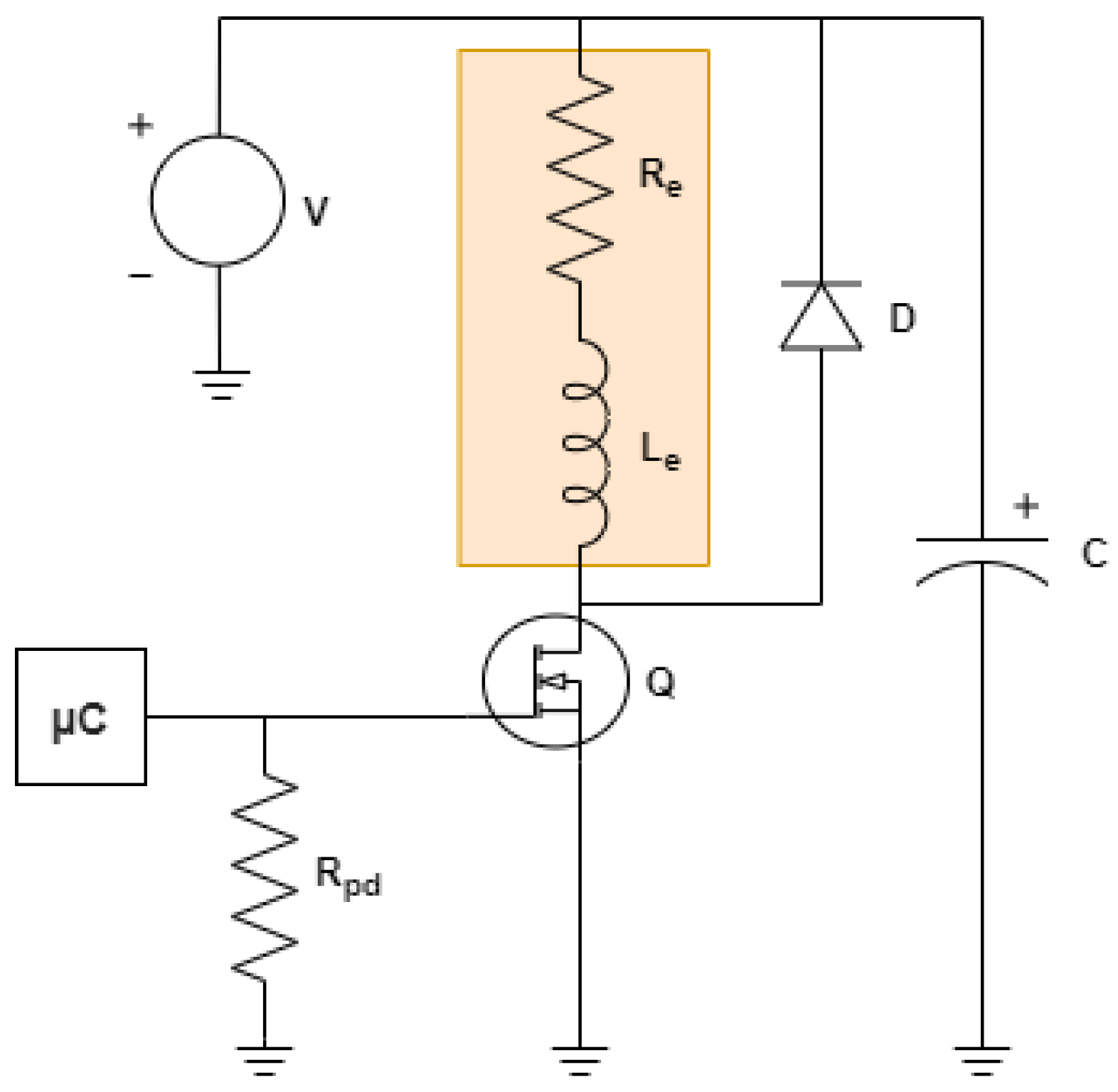
Applsci 11 02535 g001
Figure 2. Driver circuit.
Applsci 11 02535 g002
Figure 3. Position sensor and electromagnet arrangement.
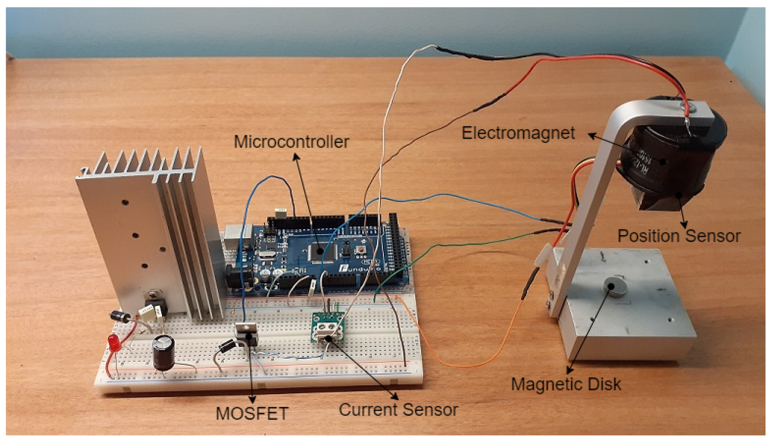
Applsci 11 02535 g003
Figure 4. Experimental electromagnetic system.
Applsci 11 02535 g004
Figure 5. Eletromagnetic system.
Applsci 11 02535 g005
Figure 6. Influence of the current on both sensors.
Applsci 11 02535 g006
Figure 7. Influence of the distance on the position sensor.
Applsci 11 02535 g007
Figure 8. Response to step input of the linearized system with both classic controllers.
Applsci 11 02535 g008
Figure 9. Simulink diagram used to test the classical controllers.
Applsci 11 02535 g009
Figure 10. Real system responses with both classical controllers.
Applsci 11 02535 g010
Figure 11. Random reference and system response with the lead–lag controller.
Applsci 11 02535 g011
Figure 12. Control signal for the random reference with the lead–lag controller.
Applsci 11 02535 g012
Figure 13. Identification network.
Applsci 11 02535 g013
Figure 14. Comparison between the system and the network responses.
Applsci 11 02535 g014
Figure 15. Inverse model controller diagram.
Applsci 11 02535 g015
Figure 16. Inverse model network - 1th5s5d.
Applsci 11 02535 g016
Figure 17. Responses of the real system when controlled by the 1th5s5d network.
Applsci 11 02535 g017
Figure 18. System response with the inverse model controllers.
Applsci 11 02535 g018
Figure 19. Comparison of system responses with lead–lag compensator and the inverse model with adaptive block.
Applsci 11 02535 g019
Figure 20. Diagram of the internal model controller.
Applsci 11 02535 g020
Figure 21. Simulink diagram of the internal model controller.
Applsci 11 02535 g021
Figure 22. Comparison of system responses with the inverse model with adaptive block and internal model.
Applsci 11 02535 g022
Figure 23. Control signal applied by the inverse model with adaptive block and internal model for the sinusoidal reference.
Applsci 11 02535 g023
Figure 24. Diagram of the model reference controller.
Applsci 11 02535 g024
Figure 25. Random reference and system response with the inverse model controller with adaptive block.
Applsci 11 02535 g025
Figure 26. Control signal for the random reference applied by the inverse model controller with adaptive block.
Applsci 11 02535 g026
Figure 27. Reference model controller network.
Applsci 11 02535 g027
Figure 28. Simulink diagram of the model reference controller.
Applsci 11 02535 g028
Figure 29. Comparison of the system responses with the internal model and reference model controllers.
Applsci 11 02535 g029
Figure 30. Control signal applied by the reference model control for the sinusoidal reference.
Applsci 11 02535 g030
Table 1. Parameters of the system [28].
ComponentValueUnits
Resistance (Re)3.0Ω
Inductance (Le)15.0mH
Maximum current1.5A
Weight (m)3.0g
Diameter37.3mm
Thickness28.5mm
Table 2. Specifications of the ATmega2560 [29].
ParameterValueUnits
Operating Voltage5V
Clock Frequency16MHz
Flash Memory256KB
SRAM8KB
EEPROM4KB
Table 3. Sensors constants.
ConstantValueUnits
α508ADU
β1090ADUcm3
γ68.274ADU/A
m29.569ADU/A
b516ADU
Table 4. Optimization of the sensor constants.
z (cm)ADCi (ADU)ADCz (ADU)icalc (A)zcalc (cm)zoptim (cm)|z-zcalc| (cm)|z-zoptim| (cm)
2.3405246150.2672.2332.2360.1070.104
2.6705305990.4612.7252.7030.0550.033
2.8705335950.5592.9062.8700.0360.000
3.1505385940.7213.1153.0550.0350.095
2.3405165920.0002.2892.3400.0510.000
3.1505165430.0003.0843.1500.0660.000
Total0.3490.232
Table 5. Optimized sensor constants.
ConstantValueUnits
α507.045ADU
β1123.801ADUcm3
γ69.474ADU/A
m30.084ADU/A
b516.343ADU
Table 6. Mean Squared Error (MSE) after training.
NetworkMSENetworkMSE
3d5n 8.8604 × 10 4 10d5n 8.0709 × 10 4
3d10n 8.7738 × 10 4 10d10n 7.8236 × 10 4
3d15n 8.6531 × 10 4 10d15n 7.7818 × 10 4
5d5n 8.7772 × 10 4 15d5n 7.5261 × 10 4
5d10n 8.3748 × 10 4 15d10n 7.3700 × 10 4
5d15n 8.1346 × 10 4 15d15n 7.0542 × 10 4
Table 7. MSE of the best identification networks for different references.
NetworkMSE StepMSE SinusoidMSE SawtoothTotal
10d5n 2.5969 × 10 4 9.0931 × 10 4 6.6006 × 10 4 1.8291 × 10 3
10d10n 2.5293 × 10 4 8.7981 × 10 4 6.6029 × 10 4 1.7930 × 10 3
10d15n 2.5085 × 10 4 8.8896 × 10 4 6.6100 × 10 4 1.8008 × 10 3
15d5n 2.4060 × 10 4 8.7159 × 10 4 6.9810 × 10 4 1.8103 × 10 3
15d10n 2.4077 × 10 4 8.9053 × 10 4 6.9631 × 10 4 1.8276 × 10 3
15d15n 2.4030 × 10 4 8.9365 × 10 4 6.9988 × 10 4 1.8338 × 10 3
Table 8. MSE obtained by the inverse model control networks for the different reference signals.
NetworkMSE StepMSE SinusoidMSE SawtoothTotal
1th5s5d 2.1019 × 10 5 1.5618 × 10 4 3.0189 × 10 4 4.7908 × 10 4
1th10s5d 2.0237 × 10 5 1.5752 × 10 4 3.0275 × 10 4 4.8050 × 10 4
1th15s5d 2.7159 × 10 5 1.5577 × 10 4 3.0127 × 10 4 4.8420 × 10 4
1th5s10d 9.8642 × 10 5 2.6887 × 10 4 5.2893 × 10 4 8.9644 × 10 4
1th10s10d 9.8300 × 10 5 2.7111 × 10 4 5.2967 × 10 4 8.9908 × 10 4
1th15s10d 1.9305 × 10 2 2.8199 × 10 4 2.5666 × 10 2 4.5253 × 10 2
Table 9. Integral Square Error (ISE), the Integral Absolute Error (IAE), and the Integral Time Absolute Error (ITAE) values for the inverse model controllers.
StepSineSawTotal
ISEInverse Model2.26811.41032.22405.9024
Inverse Model + Adaptive Block0.11660.18190.18840.4869
IAEInverse Model9.33126.82338.843224.9977
Inverse Model + Adaptive Block1.08822.04571.64444.7783
ITAEInverse Model185.3760139.8848165.4900490.7508
Inverse Model + Adaptive Block18.236538.615329.891685.7434
Table 10. ISE, IAE and ITAE values for the lead–lag and the Inverse model with adaptive block.
StepSineSawTotal
ISElead–lag1.68282.24842.29686.228
Inverse Model + Adaptive Block0.11660.18190.18840.4869
IAElead–lag8.04359.02569.150226.2193
Inverse Model + Adaptive Block1.08822.04571.64444.7783
ITAElead–lag161.1860179.8254184.7707525.7821
Inverse Model + Adaptive Block18.236538.615329.891685.7434
Table 11. ISE, IAE and ITAE values for the inverse model and the internal model controller.
StepSineSawTotal
ISEInverse Model + Adaptive Block0.45310.30030.28001.0334
Internal Model0.49500.21930.24460.9589
IAEInverse Model + Adaptive Block3.54592.68972.53248.768
Internal Model3.93832.48082.41008.8291
ITAEInverse Model +Adaptive Block72.560253.481850.2659176.3079
Internal Model76.473549.034948.2459173.7543
Table 12. MSE obtained by the reference model controller for the different signals.
ReferenceMSE
Training 2.5257 × 10 3
Step 1.0413 × 10 3
Sawtooth 1.7806 × 10 3
Sinusoid 2.2322 × 10 3
Table 13. ISE, IAE, and ITAE values for the internal model and the model reference controller.
StepSineSawTotal
ISEInternal Model0.49500.21930.24460.9589
Model Reference0.07860.12730.14470.3506
IAEInternal Model3.93832.48082.41008.8291
Model Reference0.91261.67561.39503.9832
ITAEInternal Model76.473549.034948.2459173.7543
Model Reference16.891332.202627.235576.3294
Publisher’s Note: MDPI stays neutral with regard to jurisdictional claims in published maps and institutional affiliations.

