1. Introduction
For many years, designing broad bandwidth antennas has been of significant interest to meet ever increasing demand for a high data rate in wireless communication. In theory, the bandwidth is proportional to the antenna aperture size [
1,
2]. However, in the mobile device industry, the allowed antenna volume is often limited by the requirement of mechanical stability and industrial design. For this reason, an inverted-F antenna (IFA) became a commonly used compact design due to its ease of integration and omnidirectional radiation characteristic [
3,
4]. There is still a strong demand to increase bandwidth for a given volume. Many useful techniques come from the change in antenna geometry [
5], ground plane [
6], capacitive loading with several conductive parasitic patches [
7], impedance matching circuit [
8], substrate permittivity [
9], metal chassis [
10], etc. However, little has been done in designing an IFA to improve bandwidth using an optimization algorithm.
There are many algorithmic methods for optimizing antenna geometries. These optimization algorithms are mainly classified into three categories—deterministic, metaheuristic (or stochastic), and surrogate model-assisted algorithms [
11]. The deterministic algorithms compute each iteration in a search space and find an optimal solution by simply following a simple line based on the previous iteration of best fitness. For this reason, it has a high possibility to become stuck in local maxima or minima [
12]. By comparison, the stochastic algorithms utilize random generation of possible solutions at each iteration to increase the chance of exploring the entire search space. These algorithms are further categorized as swarm intelligence-based (SI-based) [
13,
14] or non-swarm intelligence-based (non-SI-based) [
15,
16] algorithms. The key factor for success in these algorithms is heavily dependent on how thoroughly the search space is explored. Finally, the surrogate model-based algorithms build a substitutional model with multiple pre-simulated data sets to predict solutions [
17]. Examples include space mapping [
18], shape-preserving response prediction [
19], and artificial neural network (ANN) [
20].
The SI-based algorithms are bio-inspired evolutionary algorithms and beneficial in the design case where a traditional mathematical method may fail. The genetic algorithm (GA), ant colony optimization (ACO), and particle swarm optimization (PSO) are the mainstream in antenna design. These algorithms utilize a collection of agents traversing the solution space of a cost function, sometimes called the fitness function. An agent’s position in the solution space represents a set of parameters in the cost function. An agent’s cost is the fitness function evaluated at that agent’s position. The objective of GA, ACO, and PSO is to find the global maximum or (in usual practice) global minimum of the cost function. GA does this by utilizing the principles of natural biological evolution and relying on the process of selection, crossover, and mutation [
21]. In this process, only ‘elite chromosomes’ with the lowest costs survive when minimizing. The probability of survival varies with generation and the number of crossovers and mutations. ACO and PSO, by comparison, exploit the behavior of biological entities. ACO mimics the behavior of a colony of foraging ants to seek the path or position that best satisfies the cost function [
22,
23]. Some implementations of ACO mimic pheromones to urge agents towards promising solutions [
22]. PSO imitates the behavior of a swarm of flying bees looking for food [
24]. It does not exchange materials with other particles. Instead, a particle is influenced by its current position, swarm best position, and velocity. The particles are persistent and are not removed throughout the optimization process.
Recently, PSO has been utilized in a wide variety of applications in the field of antennas and electromagnetic structures. One such example is the design of novel electromagnetic materials such as phase-correcting structures [
25], artificial magnetic conductors [
26], and dielectric lenses [
27]. Of particular note is PSO’s use in antenna gain or return loss bandwidth enhancement [
28,
29,
30,
31,
32,
33]. In our study, the −10 dB return loss bandwidth of an IFA antenna is enhanced by activating or deactivating a set of conductive parasitic patches and does not depend on the reproductive process of GA’s. Thus, the PSO with binary variables (so called BPSO [
14]) was chosen for this study.
The first BPSO algorithm was developed by the original creators of the PSO, Kennedy and Eberhart [
14]. This method utilizes the same basic process as their original PSO [
24], but the particle velocity probabilistically determines whether each binary variable changes. This is done by converting the velocity into a probability via the sigmoid function. This probability determines the likelihood of a bit change in a particle’s position vector. This algorithm is commonly used in applications where the domain is discretized, and the degrees of freedom can only assume values of 0 or 1 [
31,
32,
34,
35,
36]. Other BPSO algorithms have also emerged, such as Quantum BPSO (QBPSO) [
37] and Artificial Immune System BPSO (AIS BPSO) [
38], which is claimed to produce improved results over the original version [
39]. AIS BPSO is especially attractive because both the position and the velocity of the particles are represented as strings of binary digits. In the original BPSO, distances are calculated via arithmetic operations on real numbers. AIS BPSO instead calculates velocities as the Hamming distance using Boolean operations on binary strings, allowing particles to traverse the discretized problem space more effectively. This method of optimization has already found applications in the area of antenna design [
40,
41,
42,
43,
44,
45]. AIS BPSO is promising due to its fast convergence, however, when applied to the antenna design it was found to be highly susceptible to converging to local minima [
42].
In this paper, a novel form of BPSO is proposed to configure conductive parasitic patches of an IFA for bandwidth improvement, in addition to demonstrate the effectiveness of the evolutionary optimization algorithm in limited ground clearance areas. Here, the AIS BPSO algorithm was modified by introducing a dynamic weighting factor, creating an algorithm that effectively traverses the solution space without significant sacrifice in accuracy or convergence speed. This algorithm is termed the Dynamic Hybrid BPSO (DH-BPSO). In
Section 2, we describe the operation of the DH-BPSO algorithm. In
Section 3.1, we benchmark the algorithm’s performance on common test functions, compare it with other AIS algorithms, and describe the results. In
Section 3.2, we apply the algorithm to design an IFA antenna. This is followed by fabrication of the designed antenna and verification of simulated results in
Section 3.3. Finally,
Section 4 presents the conclusion, discussion of results, and possible topics for future work.
2. Materials and Methods
The DH-BPSO algorithm includes three key components—a minimum velocity parameter, a maximum velocity parameter, and a novel weighting factor. First, the minimum velocity parameter ensures at least one bit in a particle’s position vector is flipped if the particle’s velocity is calculated to be 0. The purpose of this is to encourage particles to continue searching if they reach the swarm’s best location, so that nearby locations are also tested. Secondly, the maximum velocity parameter, originally proposed in [
38], limits the maximum number of bits in the position vector that can change between iterations. Limiting particle velocities promotes a more granular exploration of the solution space. The third component is a dynamic weighting factor distinct to the DH-BPSO algorithm.
To understand the third component, we must first distinguish the global best (Gbest) and local best (Lbest) approaches. In a Gbest approach, the velocity of each particle is calculated as a combination of the global best position and the personal best position. The global best position is the position with the lowest cost encountered by any particle in the swarm. The personal best position of a particle is the position of lowest cost encountered by that particular particle. In a Lbest approach, however, the global best position is replaced with the local best position, which refers to the lowest-cost position among a particle and its
k neighboring particles. In the array of particles that represent the swarm, the
k neighbors of particle of index
i are those particles with indices ranging from
i −
k/2 to
i +
k/2 (array wraps if
i +
k/2 is greater than the population size). In this case,
k was chosen to be two, because this neighborhood size was found to be resistant to convergence to local minima in the original study by Eberhart and Kennedy [
24]. An Lbest algorithm converges more slowly but is less likely to become trapped in local minima.
The last and most important component of the DH-BPSO algorithm is the Dynamic Hybrid Weighting (DHW). The main purpose of the DHW is to provide a balance between the Lbest and Gbest approaches. In the early iterations, the particles will mostly move towards the Lbest position, but the weighting is introduced and shift towards the Gbest position after each iteration. The result is a search that explores many possibilities at the beginning but converges quickly after finding the best area.
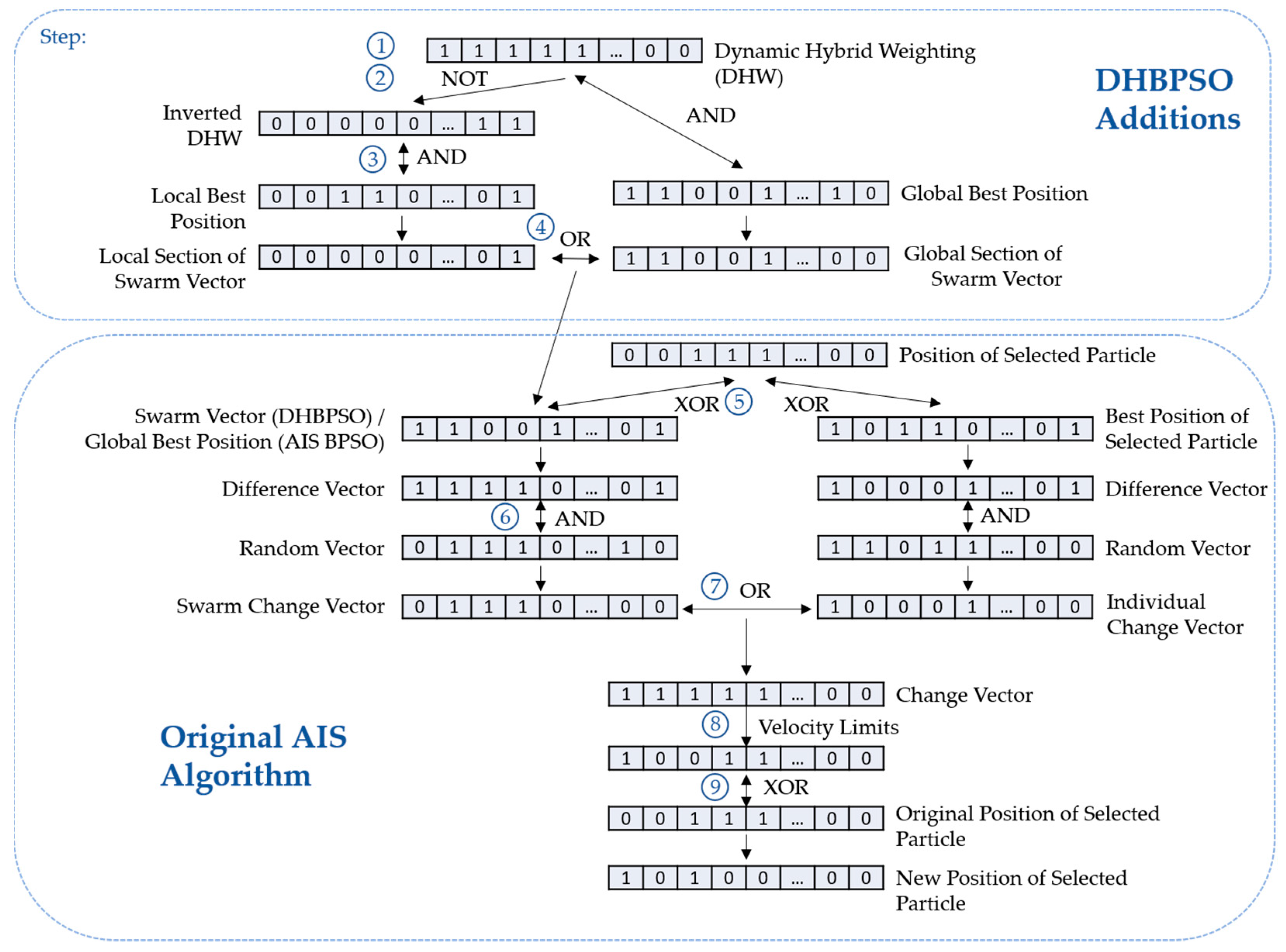
The process of the DH-BPSO algorithm is shown in
Figure 1. In step 1, the DHW vector is pseudo-randomly generated. Each bit
j of the DHW is determined by the following equations:
where rand(0,1) produces a pseudo-randomly generated decimal number between 0 and 1. The variable
in Equation (1) is the probability that the
jth bit in the DHW will be 0, as shown in Equation (2). It varies linearly with iteration, starting at 1 at the first iteration and progressing to 0 as the iteration number approaches the max iteration.
The logic used to produce the Swarm Vector from the proposed DHW is illustrated in steps 2 to 4 in the upper section of
Figure 1. The logic takes the form of a multiplexer equation with the DHW bits serving as the select bit. Specifically,
where
is the negation (NOT) operator, ∧ is the conjunction (AND) operator, and ∨ is the disjunction (OR) operator. Interpreting Equation (3), each bit of the Swarm Vector is copied from either the Lbest position vector or the Gbest position vector, depending on the value of the corresponding bit in the DHW vector. A 0 bit in the DHW vector means the corresponding bit in the Swarm Vector will be copied from the Lbest position vector. In the reverse case of a DHW bit of 1, the corresponding Gbest bit is copied into the corresponding bit position in the Swarm Vector. The Swarm Vector can also be interpreted as a weighted superposition of the Lbest and Gbest positions.
Steps 5 through 9 in the lower section of
Figure 1 show the original AIS BPSO algorithm. This is kept the same for the DH-BPSO, only replacing the global best position with the Swarm Vector. Following the logic shown on the left of
Figure 1, the difference vector
d in Equation (4) is the exclusive disjunction (XOR) between the original position of a particle
xi and the Swarm Vector in step 5. Thus,
where
denotes the exclusive disjunction operation. The position of the 1 bits in this vector correspond to differing bits between the particle’s current position
xi and the Swarm Vector.
In step 6, the 1 bits are randomly removed from the difference vector
d by taking the conjunction of the difference vector
d and a pseudo-random vector
r of 0s and 1s. This yields the Swarm Change Vector.
If the Swarm Vector in Equation (4) is replaced with the best position of the individual particle, the logic along the bottom right side of
Figure 1 will apply, and Equation (5) will then result in the Individual Change Vector. The disjunction of the Swarm Change Vector and Individual Change Vector is taken in step 7. The result is a series of bits where the 1s indicate bits to be flipped from the original position and is known as the Change Vector—the functional equivalent of a particle’s velocity. Hence,
Before calculating a particle’s new position, velocity limits set by the minimum and maximum velocity parameters are enforced in step 8. If the number of 1s in the Change Vector is between the minimum and maximum velocity parameters, the particle position is updated as usual. If the number is under the minimum velocity, random 0s are flipped until the condition is satisfied. Conversely, if the number is over the maximum velocity, random 1s are flipped. Finally, the new position of the particle
xi+1 is found in step 9 by taking the exclusive disjunction of the Change Vector and the particle’s current position
xi. Finally,
This DH-BPSO algorithm is executed using the IronPython2.7 interpreter built in to ANSYS HFSS.
4. Discussion
A new DH-BPSO was developed as a modification of the original AIS algorithm by introducing the DHW. DH-BPSO exhibited an affinity in optimizing complex, varying functions such as the Eggholder and Holder Table 2 functions. Its performance exceeded that of its AIS Hybrid, Gbest, and Lbest counterparts in terms of minimum cost achieved and iterations required to reach a minimum cost. Thus DH-BPSO has advantages in both speed and efficiency when solving problems with many satisfactory solutions and where iterations are computationally demanding. Future work may explore the effectiveness of non-linear, higher-order weightings on certain types of problems. For example, an exponential or quadratic weighting strongly favoring a Lbest approach may make DH-BPSO better suited for large domain problems with a variety of solutions.
A drawback of DH-BPSO is its dependence on the maximum iterations shown in Equation (1). For small values of the maximum iteration, DH-BPSO would quickly transition to a Gbest approach and would lose the benefit of the explorative Lbest approach. Thus, a possible avenue of research is a dynamic weighting scheme that does not depend on the maximum iteration but possibly adapts to the current speed of convergence, which could be determined from the slope of its convergence trace.
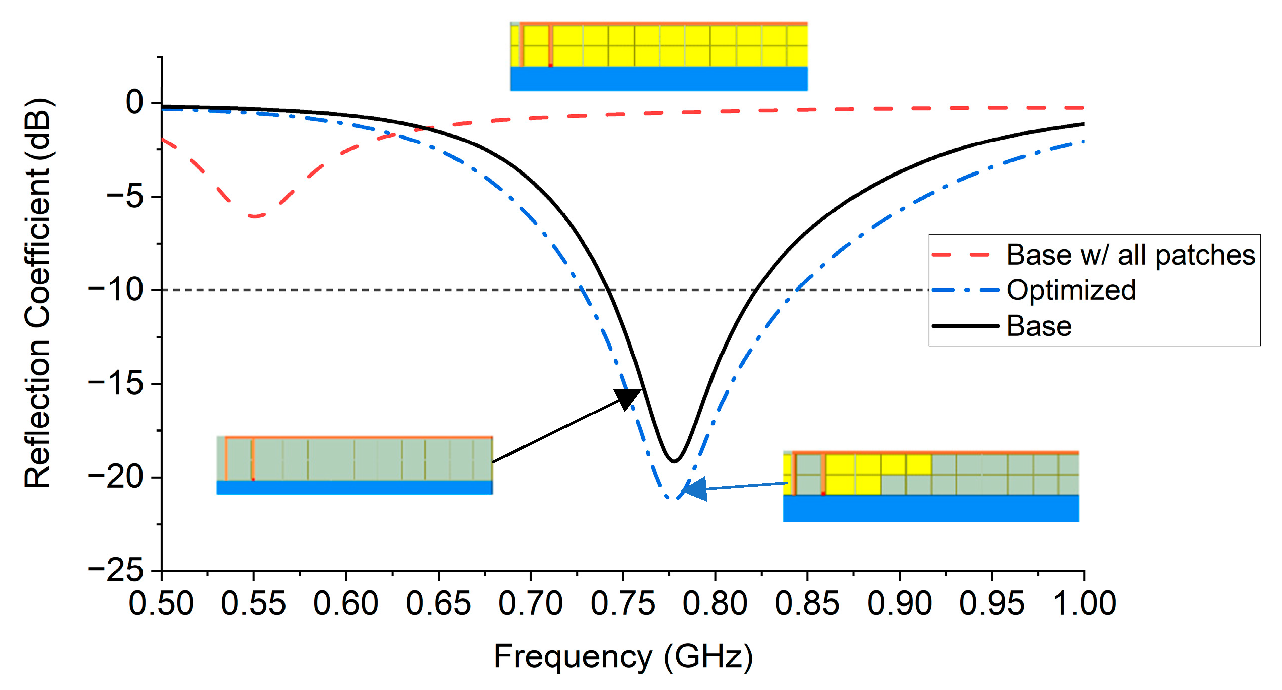
Experiments with IFA optimization show the applicability of DH-BPSO. Both measurements and simulations show an improvement in the −10 dB bandwidth, the peak gain, and the efficiency when optimized via DH-BPSO. Optimizations with this algorithm improved simulated bandwidths by as much as 74.3% and measured bandwidths by as much as 58.6%. Bandwidth improvements could be improved by further pixelating the ground clearance area, simultaneously decreasing the patch size and increasing the number of parasitic patches. This would facilitate finer control of the antenna configuration by the algorithm, possibly allowing for better solutions with wider bandwidths.
Although this paper only considered the IFA, the process can be easily applied to other antenna geometries such as patch, slot, and loop antennas. The parasitic patches can be configured around each antenna as previously done, and the number of dimensions of the optimization can be increased appropriately. This will lead to a longer convergence time, but in theory the number of parasitic patches can be increased indefinitely with appropriate time and computing resources.
Another potential future area of work is extending DH-BPSO to find solutions to multi-objective problems. For example, the radiation pattern could be analyzed in addition to bandwidth. Additionally, desired resonant frequencies may be incorporated into the cost function to ensure increased bandwidth in a frequency band of interest. The principle of a dynamic weighting factor can also be applied beyond just the AIS BPSO to any PSO that incorporates local and global best approaches.


