Article

An Improved VGG19 Transfer Learning Strip Steel Surface Defect Recognition Deep Neural Network Based on Few Samples and Imbalanced Datasets

Shanghai Key Laboratory of Intelligent Manufacturing and Robotics, Shanghai University, Shanghai 200444, China
*
Author to whom correspondence should be addressed.
Appl. Sci. 2021, 11(6), 2606; https://doi.org/10.3390/app11062606
Submission received: 14 January 2021 / Revised: 9 March 2021 / Accepted: 11 March 2021 / Published: 15 March 2021
(This article belongs to the Section Applied Industrial Technologies)

Abstract

:
The surface defects’ region of strip steel is small, and has various defect types and, complex gray structures. There tend to be a large number of false defects and edge light interference, which lead traditional machine vision algorithms to be unable to detect defects for various types of strip steel. Image detection techniques based on deep learning require a large number of images to train a network. However, for a dataset with few samples with category imbalanced defects, common deep learning neural network training tasks cannot be carried out. Based on rapid image preprocessing algorithms (improved gray projection algorithm, ROI image augmentation algorithm) and transfer learning theory, this paper proposes a set of processes for complete strip steel defect detection. These methods achieved surface rapid screening, defect feature extraction, sample dataset’s category balance, data augmentation, defect detection, and classification. Through verification of the mixed dataset, composed of the NEU surface dataset and dataset in this paper, the recognition accuracy of the improved VGG19 network in this paper reached 97.8%. The improved VGG19 network performs slightly better than the baseline VGG19 in six types of defects, but the improved VGG19 performs significantly better in the surface seams defects. The convergence speed and accuracy of the improved VGG19 network were taken into account, and the detection rate was greatly improved with few samples and imbalanced datasets. This paper also has practical value in terms of extending its method of strip steel defect detection to other products.

1. Introduction

1.1. The Significance and Development of Strip Surface Defect Detection

Strip steel is one of the main products of the iron and steel industry. It is an indispensable raw material of shipbuilding, automobiles, machinery manufacturing and other industries. The quality of strip steel will directly affect the final product’s quality and performance. In the strip steel manufacturing process, due to various factors such as raw materials, rolling equipment, and processing techniques, the surface of strip steel can develop different types of cracks, scarring, holes and other defects [1]. Strip steel surface defects not only cause serious production accidents such as strip breaking, stacking, and production line downtime, but also cause serious roll wear, with an immeasurable economic and social influence on the production enterprise [2]. More than 60% of strip steel product user quality objection events in China are caused by surface defects. Therefore, it is very important to improve the quality of strip steel by detection of these defects in the rolling process in time, adjustment of control parameters, classification, and labeling of different strip steel levels.
In traditional iron and steel enterprises, the surface quality of high-speed moving strip steel is usually detected by an artificial naked eye stroboscopic method. However, this method also has its shortcomings. For example, stroboscopic lighting can only be used on some specific strip surfaces. Due to visual fatigue, detection timeliness is poor, and the missed detection and misdetection rate are high. For products surface defect detection carried on a conveyor belt, the human eye can detect only 60% of the surface defects, and the width of the product cannot exceed 2 m and, the moving speed of the products cannot exceed 30 m/s, in the best case [3]. At present, many Chinese metallurgical enterprises still use manual visual inspection and sampling inspection of strip steel surfaces with low efficiency and poor detection efficiency.
In recent years, with the development of industrial technology, machine vision is gradually being used more often in enterprises as a non-contact and non-destructive testing technology. Machine vision has a high resolution, is highly classified, is little affected by the ambient electromagnetic field, and is low cost. By deploying the image acquisition apparatus online and sending the real-time collection images to a monitoring device, inspectors can achieve real-time monitoring of the metal surface.

1.2. The Practical Difficulties of Using the Machine Vision Surface Detection Technique on Imbalanced Datasets

The key to machine vision surface detection technique is developing various types of defect detection algorithms. Due to strip steel’s rapid movement on the production line, it will produce a large amount of image data (for example, 25 frames/sec), which demands an excellent real-time defect detection algorithm. It also can lead images captured by CCD cameras to be of low resolution and less qualified. Since the defect images captured by CCD cameras fall into numerous categories, are complex, and have boundary overlap, it is typical to have an imbalanced dataset with a small number of samples. When the data has a long-tail distribution, it can lead to bias in the classifier. The classifier is more inclined to identify classes with a sufficient sample size and rich diversity [4,5]. However, it is unfair to ignore other classes. Traditional machine learning algorithms do not have enough data, either in terms of quantity or quality, to train a model.
Standard machine learning algorithms are based on the assumption that the dataset has a sufficient number of samples and balanced class distribution. Uneven distribution in a few samples dataset causes tremendous difficulties for standard algorithm application. Algorithms prefer that the categories contain plentiful samples and that each category contains a similar number of samples.

1.3. Scope of Our Work and Contribution

Combined with previous research results, this paper proposes An Improved VGG19 Transfer Learning Strip Steel Surface Defect Recognition Deep Neural Network Based on Few Samples and Imbalanced Datasets, for strip steel defect detection. The main contributions of the paper are summarized below:
(1) For strip steel with a low defect rate, edge false defects and illumination interference, which make it difficult to extract various kinds of real defects, we present an improved strip steel surface defect detection algorithm based on gray-scale projection. The algorithm can filter out defect-free surfaces, edge false defects, and illumination interference, and extract defects on the surface effectively. The algorithm is especially effective for longitudinal cracks, transverse cracks, and large area surface defects.
(2) In view of the category imbalance problem, starting from the data level approach method, this paper proposes a data augmentation algorithm based on ROI region random crop for uneven categories, to achieve sample balance in the categories.
The remainder of this paper is organized as follows. In Section 2, we compare our work with related research, with a focus on surface defect detection algorithms and imbalanced learning algorithms. In Section 3, by the use of our improved gray projection algorithm, we undertake detector rapid screening of the strip steel surface and extract defect regions. In Section 4, our ROI image augment algorithm augments smaller classes and makes images balance again using the data level approach method. In Section 5, the improved transfer learning deep neural network based on VGG19 detects and identifies the few samples and imbalanced strip steel dataset. In Section 6, we compare the real-time performance between our network and some deep learning detection algorithms. Section 7 concludes this paper with some future research directions. In Figure 1, we present the overview of the strip steel defect detection method of this paper.

2. Related Work

2.1. Categories of Surface Defect Detection Algorithms

According to Author [6], surface defect detection algorithms can be divided into four categories: traditional statistical-based algorithms, spectrum-based algorithms, model-based algorithms, and emerging deep learning algorithms. For deep learning algorithms, three are traditional defect detection algorithms. Only two-dimensional defect detection algorithms are discussed in this paper.
For traditional defect detection algorithms, for example edge detection [7], gray level statistics [8], local binary pattern [9], wavelet transform [10], genetic algorithms [11], and the fractal dimension model [12], features are extracted by manually designed feature extractors, then the features are learned by various feature classifiers, such as K nearest neighbors [13], support vector machine [14,15], Random Forest [16], etc. However, the robustness and real-time performance of these traditional algorithms are poor. The processes of data pre-processing, feature extraction, feature reduction, and classifier selection in traditional algorithms need the experience of experts. When images contain noise or textured backgrounds, the real defect edges may be missed due to noise interference, which does not meet the requirements of on-line detection of surface defects.
With the rapid development of artificial intelligence, a computational vision of surface defect recognition and classification has emerged. Convolutional neural networks (CNNs), as a typical deep neural network (DNN), have been widely used in the fields of fault diagnosis, defect detection, and image recognition. Author [17] proposed a Max-Pooling convolutional neural network. Compared to the performance of SVM classifiers, the Max-Pooling convolutional neural network performs at least two times better. Author [18] proposed a semi-supervised learning method using a convolutional neural network (CNN). The proposed method requires fewer labeled samples, and the unlabeled data can be used for training. Author [19] proposed an improved You Only Look Once (YOLO) network. The network achieved a 99% detection rate with speed of 83 FPS on 4655 digital photos of steel strip surfaces.
Due to the limitation of data size, it is difficult for large baseline CNNs to be fully trained. Thanks to transfer learning and ImageNet’s pre-training networks, it is feasible to train few samples datasets on large baseline CNNs by fine-tuning networks’ structures on the pre-training networks. Transfer learning is a way to learn from previous tasks and apply the learning to new tasks. Its purpose is to extract knowledge and experience from one or more source tasks, and then apply this to a new target domain. Since 1995, transfer learning has attracted the attention of many researchers. The basic unit of an image is a pixel point; different gradations of pixel point arrangements and combinations together can represent various types of low-level features, such as lines, dots, and colors. By matching and combining these low-level features with each other, high-level image information can be formed, such as texture and geometries. Although high-level information of different images is different, underlying features are similar [20]. This is the basis of image data transfer learning.
Author [21] showed that transfer learning can be successfully applied using image data from an entirely different domain. Author [22] proposed a baseline ResNet convolution neural network (CNN) with a multilevel feature fusion network (MFN) module. On the NEU database, ResNet50 with the MFN module achieves a 99.7% detection rate with a speed of 6.1 FPS. Author [23] proposed a crack detection method based on a deep fully convolutional network (FCN) with VGG16 backbones. The network achieved about 90% average precision on a subset of 500 annotated 227 × 227-pixel crack-labeled images.
Transfer learning has been successful not only in the field of computer vision, but also has many applications in industry. Author [24] proposed a deep transfer fault diagnosis framework. Author [25] proposed an acoustic event classification deep transfer learning network. In Author’s work [26], transfer learning is applied to wind power prediction. The transfer learning method not only saves time in collecting data from wind farms, but also stipulates good weight initialization points for each of the wind farm for training.
Since the VGG neural network is a linear structure and the network is classically simple, the VGG network was chosen as the backbone network for defect recognition in this paper [27]. The VGG neural network is a transfer learning network series, including VGG11, VGG13, VGG16, and VGG19. The common feature of these network structures is that several convolution layer modules are connected to three full connection layers. Finally, defects are identified and classified through a softmax layer. For example, VGG11 is composed of eight convolution layers and three full connection layers. Similarly, VGG13, VGG16, and VGG19 all contains three full connection layers. However, due to the large number of parameters in the full connection layer, three full connection layers will greatly slow down the efficiency of network training and recognition. Therefore, when the VGG network was selected as the backbone of the pre-training network in this paper, three full connection layers were removed. Compared with VGG19 and, VGG11, VGG13 and VGG16 are shallow networks. Due to the small amount of training data of the network in this paper, the recognition accuracy of the network is relatively low on the shallow network, and the convergence of the network is poor. Therefore, our network needed a fully pre-trained network on ImageNet as the backbone network, so VGG19 was chosen for the transfer learning backbone network in this paper.

2.2. Levels of Imbalanced Learning Algorithms

For few samples and imbalanced datasets, imbalanced learning algorithms have been proposed. Imbalanced learning algorithms can be divided into three main categories: the data level approach method, algorithm level approach method, and ensemble learning level method.
(1) The data level approach method is the earliest and most widely used in the field of imbalanced learning regions; it also referred to as the resampling method. Along with modifying the training dataset to fit standard learning algorithms, Mani proposed an under sampling method to delete samples from bigger categories [28]. He Bai et al. proposed an oversampling method by generating new samples for smaller classes [29]. Batista and Prati et al. proposed a mixing project in conjunction with two methods described above [30]. These methods rely on a well-defined distance measure, but industrial datasets often contain multiple non-linear features or missing values. In addition, the range of different features may be large. To define a reasonable distance measure on these datasets is very difficult, and requires tremendous extra computing resources to meet real-time requirements.
(2) The algorithm level approach method is represented by the cost-sensitive learning method; it focuses on modifying existing standard machine learning algorithms to change their preferences on major classes. In order to reduce classifier’s preference for the majority classes, this method artificially increases the importance of smaller classes in the training process [31,32]. The cost matrix of these algorithm needs to be provided by experts in the field based on prior knowledge of the task, which in many real-world problems is not achievable. Due to a lack of prior knowledge in the regions, the cost matrix cannot guarantee classification performance, and can even lead the objective function to drop into the local optimal/saddle point. However, a specific cost matrix can only be used for the task for which it was designed, and cannot be generalized to different tasks.
(3) Ensemble learning combines the data level approach method and algorithm level approach method to obtain a more powerful integrated classifier. Due to its excellent performance, ensemble learning is widely used in category imbalanced tasks [33,34]. However, ensemble learning does not always lead to a better performance. Blind retention policies for difficult to classify samples may result in over-fitting in the latter period of the iterative process. Algorithms have the advantage of high data transfer efficiency and utilization, but poor robustness against noise data.

2.3. The Development of Deep Learning on Few Samples and Imbalanced Datasets

After 2010, as the popularity of high-performance computers and hardware increased, deep learning became more widely used in industry. It provided a new way for machine vision to solve strip steel surface defect detection problem with few samples and imbalanced datasets. Based on the idea of deep learning, researchers used the algorithm level approach method to further explore this research area. Typical algorithms for this included OHEM [35] (Online Hard Example Mining), S-OHEM [36] (Stratified Online Hard Example Mining), A-Fast-RCNN [37] (Adversarial Fast Region-based Convolutional Neural Network), Focal Loss [38] and GHM [39] (Gradient Harmonizing Mechanism).
The disadvantage of the OHEM algorithm is that is only leaves samples with high loss and completely ignores simple samples, which leads the model to lose the ability to distinguish simple samples. Compared to the native OHEM algorithm, the S-OHEM algorithm avoids the disadvantage of using only high loss samples to update their model’s parameters. However, when the model is applied to different datasets, it also introduces an additional hyper-parameters problem. The A-Fast-RCNN method generates images through the GAN network. The GAN neural network is composed of two subnetworks. One subnetwork generates similar data by learning how the original data are distributed. Another subnetwork discriminates the authenticity of the generated data. In this way the GAN neural network can realize a simulation of the original data. However, for few samples datasets (each type of image only has a dozen images or less, each image is a gray-scale image of about 30~50 KB) with low-quality images, it is not enough to support the training of the GAN network. The Focal Loss method modifies its cross-entropy function to make the training process more attentive to difficult samples. The GHM continues to improve its cross-entropy function on the basis of Focal Loss. The biggest difference between the GHM algorithm and the Focal Loss algorithm is that the GHM algorithm assumes that the difficult samples are abnormal samples.
However, strip steel has a complex texture, different types of defects, different morphologies of similar defects, different types of false edge defects, and severe light interference defects. It is difficult to meet the requirements of strip steel defect detection only using the algorithm level approach method. The data level approach method and algorithm level approach method must be combined to deal with difficult samples and abnormal samples using defect detection and classification processes. Further discussion is available in Section 3.

3. Rapid Quality Screening and Defect Feature Extraction Algorithm on the Strip Steel Surface

3.1. Rapid Quality Screening Problems on the Strip Steel Surface

In the production process, the moving speed of strip steel can exceed 10 m/s, while stripping steel surface defects are small; most of the strip steel surface is without defects. In order to process large amounts of data more efficiently and rapidly, the strip steel surface online defect detection system is generally divided into two parts: rapid quality screening and defect feature extraction. Rapid quality screening detects whether images captured by CCD camera in real-time contain suspected defects, then images with suspected defects are sent for further processing and surface defect-free images are ignored. Due to the large amount of defect-free images that do not need to be processed, the number of suspected defects images is greatly reduced, not only saving time but also improving detection efficiency. For the rapid screening processing stage, algorithms are preferred for the simple and fast screen surface, rather than accurate defect localization.
At present, the most widely used algorithm for the rapid screening method is the background subtraction method, which compares target images and their background to obtain contrast images. If some pixels that have a greater value than the preset threshold, these pixels are suspected defect regions, and the defect detection system will cache these images for further screening. However, the background subtraction method in actual production suffers from the light environment, camera hardware performance and image blurring; a large number of false defect images are detected with this method. The false defect is an important part of strip steel surface defects; how to screen false defects must be considered within the scope of this paper. In the distribution of strip steel defects, the edge portion is a defect-prone region of the strip steel surface. Therefore, in order to ensure full coverage of the strip steel surface, a CCD camera captures the edge region and background image simultaneously during the image acquisition process. However, it will introduce false edge defects, so an edge region rapid screening method is the key to rapid quality screening of the strip steel surface.

3.2. Strip Steel Edge and Background Region Automatic Detection

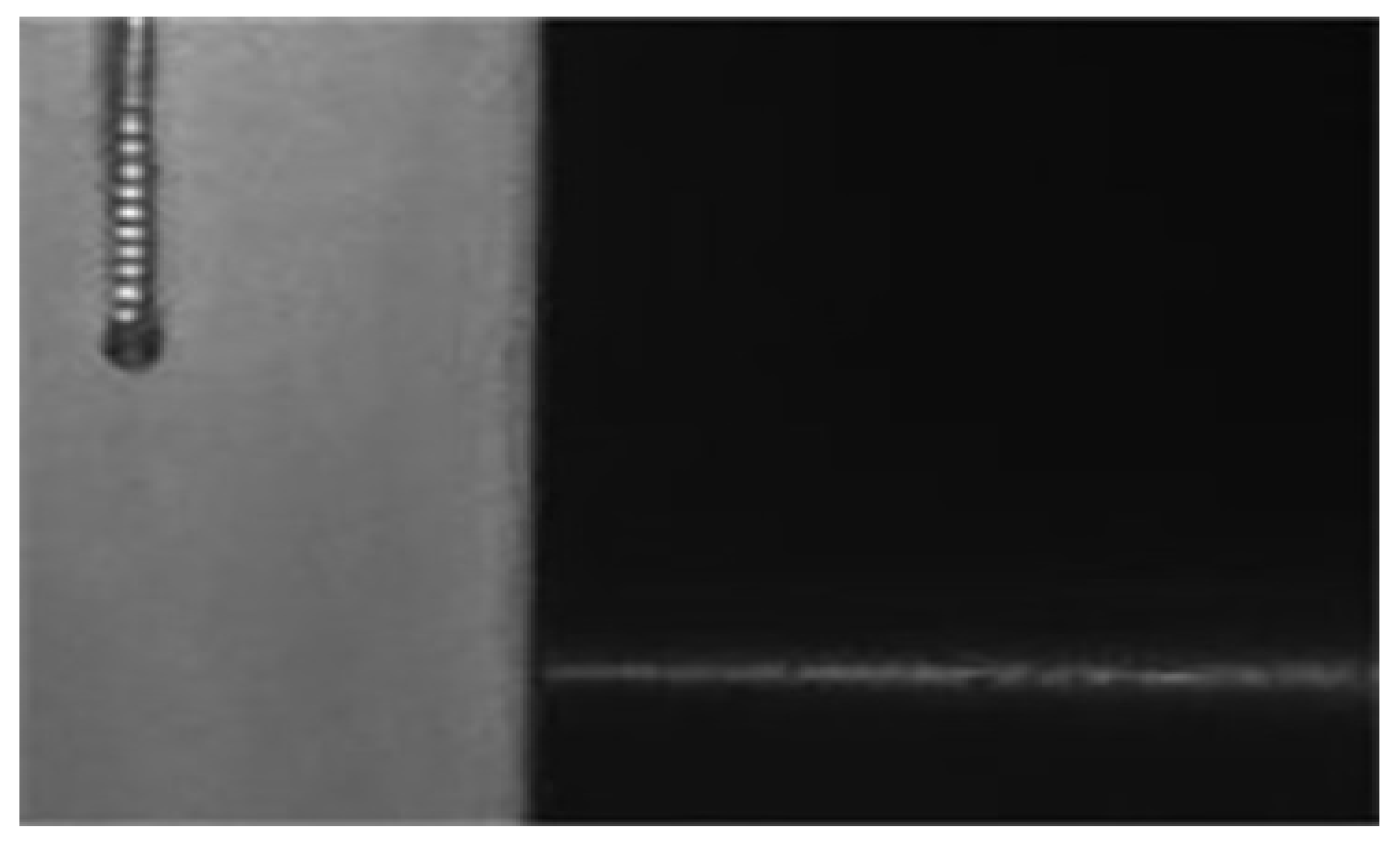
As shown in Figure 2, since there is no high reflectivity metal outside the strip steel edge region, the background is usually dark. In the background image, there is only a narrow strip steel conveying guide rail, with a relatively simple color and much lower gray-scale value than the strip steel surface. For image edge background screening questions, the average gray projection value concept was proposed. The average gray projection value is the average gray-scale value on the horizontal or vertical projection. If the image has an average gray-scale value on the horizontal or vertical projection that is too low and below a certain threshold, it is believed that this row or column is located in the background.
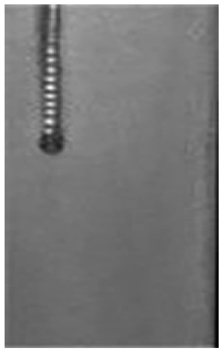
The threshold value of the average gray projection value can be pre-adjusted according to the scene illumination gradation and defect-free strip steel’s gray-scale value. The threshold value is set according to the lighting conditions of each experiment and defect-free strip steel images; it is an empirical value from a large number of comparative tests. After a simple calculation of the average gray projection value and gray-scale value comparison, the strip steel edge region and background can be substantially divided. Figure 3 shows a steel strip defect acquisition region.

3.3. An Improved Strip Steel Surface Rapid Quality Screening and Defect Feature Extraction Algorithm Based on Gray-Scale Projection

In actual production, not all images captured by CCD cameras contain a defect. In general, the defect region ratio is 5% or less (Steel Acceptance Criteria: GB.1965/1978). Therefore, rapid screening of defect-free surfaces can not only greatly decrease the amount of calculation required, but also improved detection efficiency. Influenced by scene illumination gradation and hardware devices, images captured by CCD camera will generate blurred edges or the strip steel edge may not be detected. This can contribute to an edge false defect, where the defect does not exist in practice. As shown in Figure 4, in the steel strip defect acquisition region, processed by the Canny edge detection operator, there is a significant break elongated fold line between the strip steel edge and background intersection region. If using the background subtraction method to detect the fold line, it will be misidentified as a strip steel surface defect. A large number of edge false defects pose a challenge to rapid quality screening of strip steel surfaces and defect feature extraction.
Through a lot of experiments, it has been found that false defects on the edge of strip steel have a common characteristic: the false defect edge is no longer a straight line, but a bent or broken fold line. The fold line is very narrow and close to the transform region between the strip steel edge and background. In view of the above characteristics of edge false defects, an improved strip steel surface rapid quality screening and defect feature extraction algorithm based on gray-scale projection is proposed in this paper on the basis of the background subtraction method. Considering that there are many transverse and longitudinal stripes of strip steel defects, and the system speed requirements for detection on-line, this paper only calculated the gray-scale value on horizontal and vertical projection. Firstly, the algorithm projected images horizontally and vertically. Corresponding to gray-scale value of each row and column, the algorithm calculated the maximum gray-scale values (RMax, CMax), minimum gray-scale values (RMin, CMin) and average gray-scale values (RAvg, CAvg) for each row and column, where GlobalAvg is the global average gray-scale value of the image and µ is the threshold coefficient of the defect (µ ranging from 20% to 30%). In this paper, µ was set at 30%.
(1) If the difference [CMax–CMin] between the maximum gray-scale value and minimum gray-scale value on the vertical projection is not within (1 ± μ) GlobalAvg, the column of the image is defect-free.
(2) If the [CMax–CMin] and CAvg on the vertical projection is in the range of (1 ± μ) GlobalAvg, the column of the image is a defective image.
(3) If the [CMax–CMin] in (1 ± μ) GlobalAvg, but CAvg < (1 − 2μ) GlobalAvg, the average gray projection value in this column is too low. This means the column of the image is the transform region between the strip steel edge and background.
(4) If extended two times the length of the transform region across columns, it is the false defect region.
(5) If the [CMax–CMin] is not within (1 ± μ) GlobalAvg and CAvg are much smaller (over 10 times) than the value of GlobalAvg. This means the average gray projection value of the column is too low and the column is background.
(6) If the [CMax–CMin] is not within (1 ± μ) GlobalAvg, but CAvg is 1.5 times to 2 times as much as GlobalAvg, the column of the image is a highlighted defective.
Before image pre-processing, the strip steel image should be digitally transformed into a gray-scale image. Firstly, define two one-dimensional matricews R[M] and C[N], where M, N is the number of rows and columns of the image. With the help of two arrays to store the image’s average gray-scale values on horizontal and vertical projections, the paper used the following algorithm to detect images. The pseudo-code of strip steel surface rapid quality screening and the defect feature extraction algorithm based on gray-scale projection are shown below in Algorithm 1:
Algorithm 1 Rapid Quality Screening and Defect Feature Extraction Algorithm
Input: original image matrix f(i, j), Size = M × N, iϵ[0, M − 1], jϵ [0, N − 1]
Output: ROI Defect Region
matrix R[M], Size = M × 1; empty matrix C[N], Size = 1 × N
 
Step 1. Calculate Initial Values
for int R = 0, R ≦ i, R++;   △Calculate the matrix by rows, fixed the rows first
for int j = 0; j ≦ N − 1, j++;   △Iterate through the columns of the matrix
  f(R, j), Size = M × 1
  RMax = Max(f(R, j)), Size = 1 × 1
  RMin = Min(f(R, j)), Size = 1 × 1
  RAvg = Sum(f(R, j))/M, Size = 1 × 1
  Add RAvg into R[M],
Return R[M], Size = M × 1
△The same principle is used to calculate the matrix by column to obtain C[N], Size = 1 × N
GlobalAvg[M, N] = Sum(R[M])/M  Or  Sum(C[N])/N, Size = 1 × 1
 
Step 2. Confirm Detection Region
if RAvg Or CAvg << GlobalAvg[M, N];   △The row or column is the background area
 Delect the Row or Column with low projection value
Add rest of area into Confirm Detection Region
 
Step 3. Suspected Defect Region
△region with Defect Region; Transform Region; False Defects Region
if (1 − µ) GlobalAvg[M, N] ≦ RMax − RMin ≦ (1 + µ) GlobalAvg[M, N]
Or
 (1 − µ) GlobalAvg[M, N] ≦ CMax − CMin ≦ (1 + µ) GlobalAvg[M, N]
Else if 1.5*GlobalAvg ≦ CAvg Or RAvg ≦ 2*GlobalAvg
  Find Highlighted Defective ROI Region
Add rest of area into Suspected Defect Region
 
Step 4. Detection Transform Region
if RAvg Or CAvg < (1 − 2µ)GlobalAvg[M, N];
 Find Transform Region T- Region, △region between strip steel edge and background
 Delete T- Region
 
Step 5. False Defects Region
Find the position of T- Region,
 Extend T- Region’s length twice by horizontal and vertical coordinates
 Delete False Defects Region
 
Step 6. Output
ROI Defect Region = The final remaining area + Highlighted Defective ROI Region
Get ROI Defect Region

3.4. Strip Steel Surface Rapid Quality Screening and Defect Feature Extraction Experiment

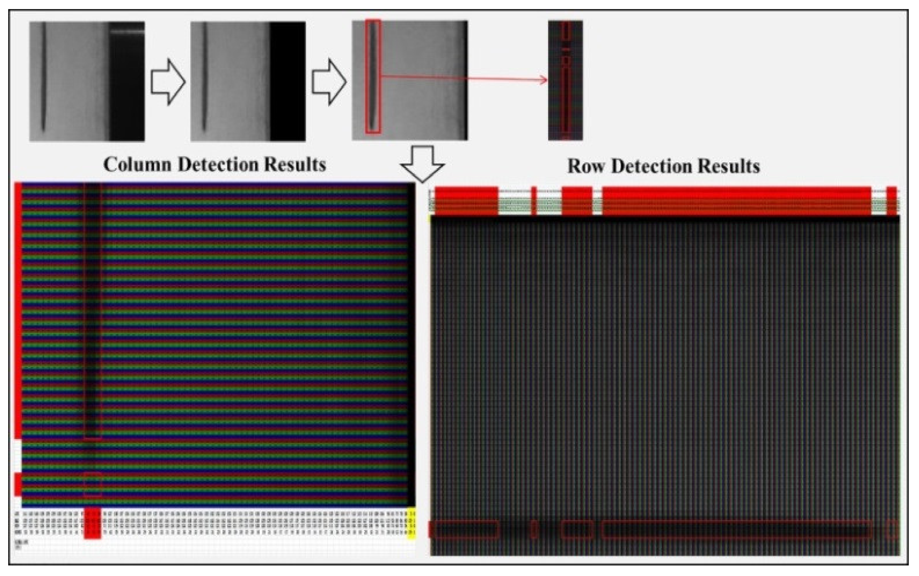
As shown in Figure 5, the strip steel defect acquisition region image in Figure 3 was transformed into a corresponding gray-scale matrix. With the help of the gray-scale projection algorithm proposed in this paper, various kinds of defect regions can be rapidly screened. The gray-scale matrix’s GlobalAvg = 111.3083, threshold value (1 ± μ) GlobalAvg is from 77.9 to 144.7.
In the yellow region, CMax–CMin = 41, CAvg = 2, the column of the image is background.
In the green region, CMax–CMin = 101, CAvg = 28.8, the column of the image is the transform region between the strip steel edge and background.
On the basis of the green region and length of the transform region across columns, extended two times the blue region is the false defect region.
In the red region, CMax–CMin = 119, 126, 111, CAvg = 103, 116, 105. Therefore, these three columns of the image are defective images.
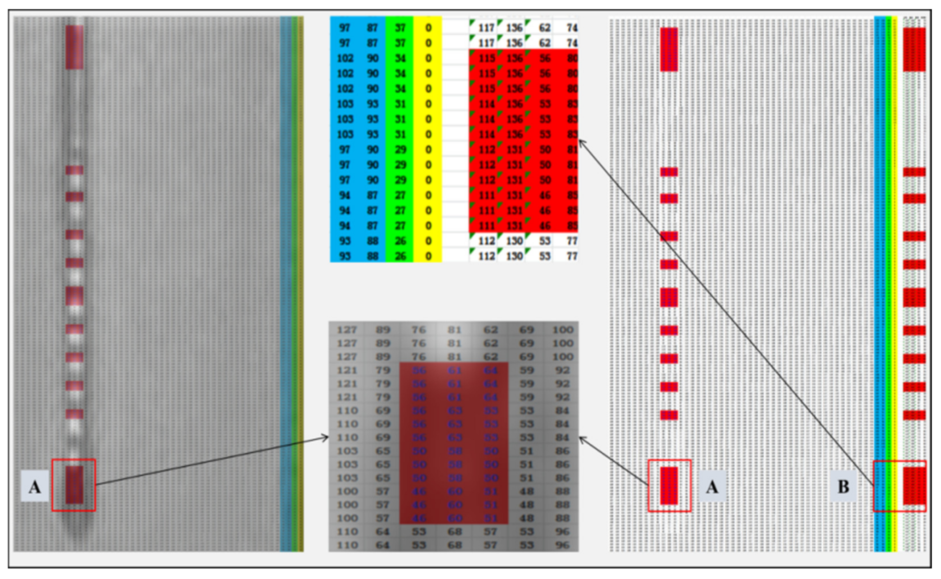
Figure 6 shows the detection result for the steel strip. Since the picture of row analysis results is too large, we enlarged the detection area A and area B to display results more vividly. In this figure, the effect of overlapping the original image and ROI area is shown on the left. The right side shows the effect of the original image analysis. In area A, the red area is the ROI area, which is exactly on the defective position of the original image. Area B is the row analysis results of the image, where RMax–RMin = 80, 80, 80, 83, 83, 83…, RAvg = 115, 115, 115, 114, 114, 114…, threshold value (1 ± μ) GlobalAvg from 77.9 to 144.7. Therefore, these 12 rows of the image are defective rows.
Similarly shown in Figure 7, our algorithm detected a longitudinal flaw image. It can be seen that our algorithm detected the defect area perfectly.
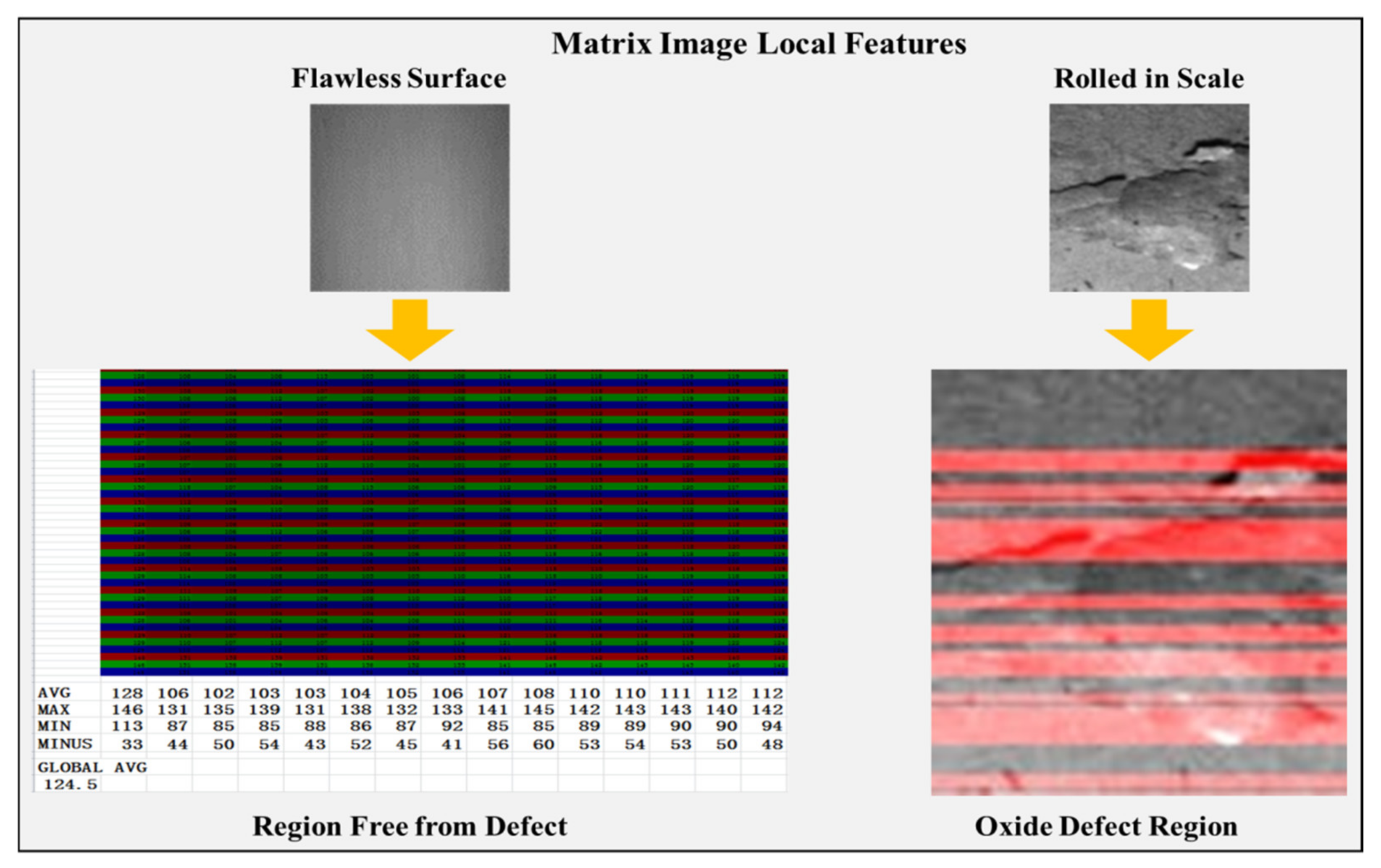
To further verify the validity of our defect detection algorithm, the algorithm was tested in an experiment comparing a flawless surface and oxide defect surface. Figure 8 shows the contrast of the improved gray-scale projection algorithm’s performance on the defect-free and defect surface. Due to the large region of the defect-free image on the left in Figure 8, only part of the calculation results are shown in this paper, while the defect region on the right image is marked in red. It can be seen that our improved gray projection algorithm can quickly screen defect and defect-free surfaces, and extract defect features.
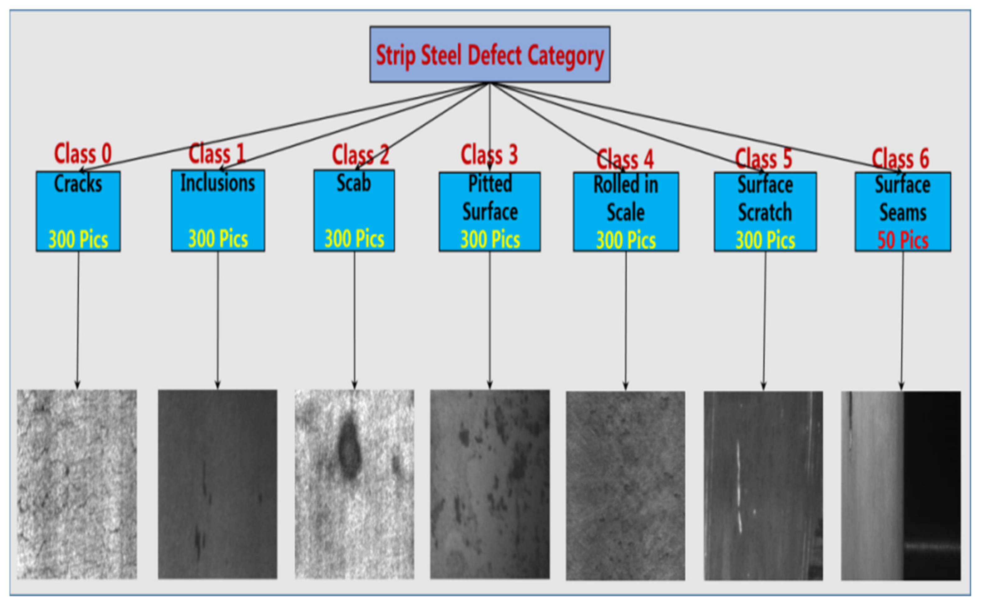
The object of study in this paper was a mixed image dataset, consisting of the NEU Surface Dataset [40] and our strip steel defect images. The NEU surface dataset contains six major types of strip defects: cracks, inclusions, scabs, pitted surfaces, rolled in scales, and surface scratches. Each category contains 300 pieces of images, for a total of 1800 pieces of images, each of which is 200 × 200 pixels. The images in the dataset are BMP format and each image is a 40.1 KB gray-scale image. On the other hand, our experimental dataset has only one category of strip steel defect called seams. This category contains 50 pieces of images and each image is a 30KB gray-scale image. As shown in Figure 9, from class 0 to class 5 is the NEU surface dataset, and class 6 is our experimental dataset.
We randomly selected 80% of the mixed dataset to test our feature extraction algorithm, and the remaining 20% of the data was used as the test data in Section 5. The defect feature extraction algorithm was implemented by using Python 3.6 and OpenCV 4.4.0. The detection time of each image was 3.5 ms (287.5FPS).
As shown in Table 1, our feature extraction algorithm is more effective for large area defects, such as longitudinal cracks, transverse cracks, surface seams, etc. However, the algorithm cannot effectively detect small area defects such as inclusions, rolled in scale, or a pitted surface.
For the defect images with high brightness background or high reflective surface, the algorithm will have some degradation in detection accuracy. For those types of defects, it is recommended to use our algorithm in a dark field lighting system.
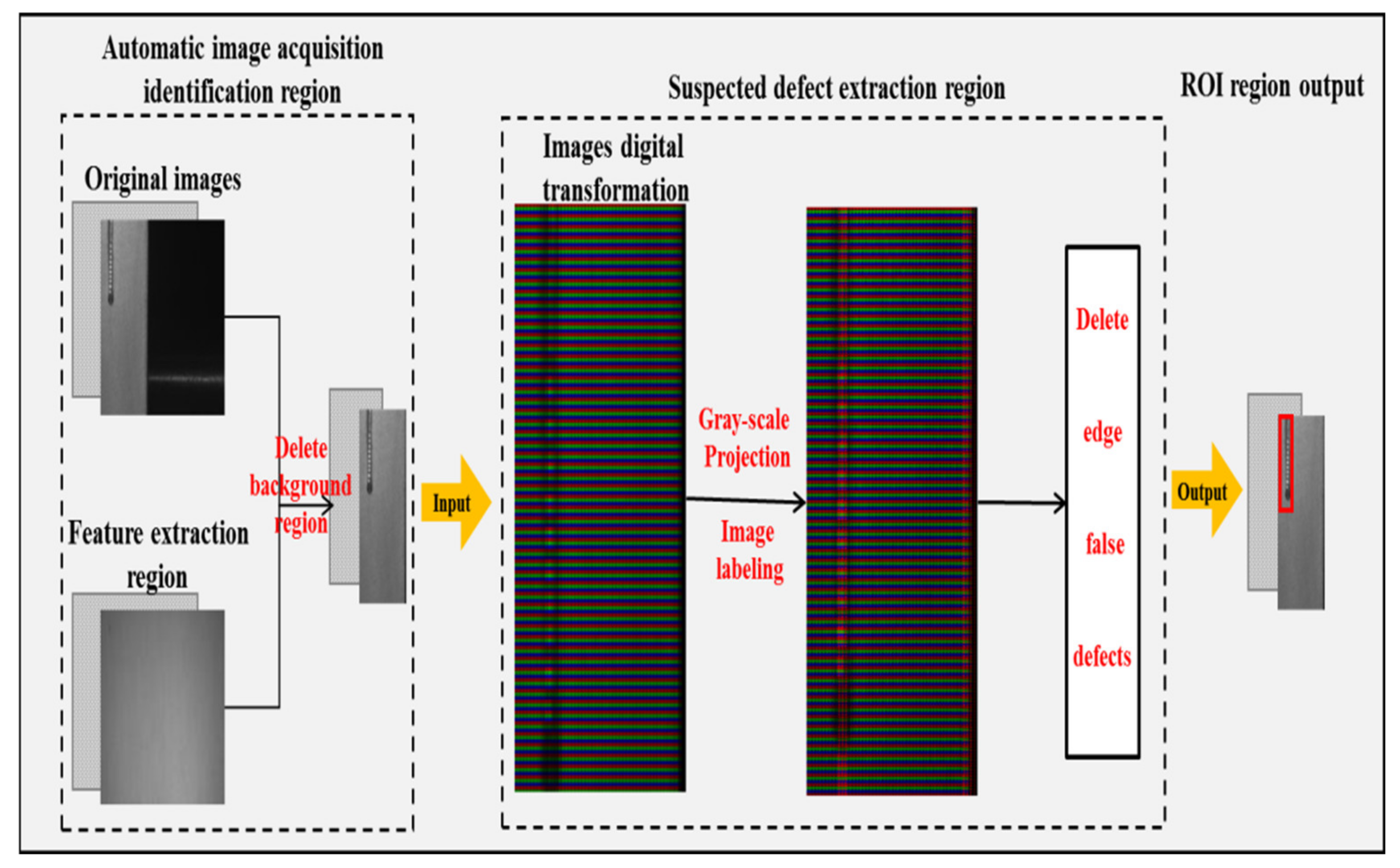
Figure 10 is the process of improved strip steel surface rapid quality screening and the defects feature extraction algorithm based on gray-scale projection. Firstly, the algorithm takes advantage of the clear distinction between the background and strip steel surface to identify images acquisition regions and automatic crop the background region. The algorithm rapidly screened the rest of strip steel surface, then extracted suspected defect region and deleted edge false defects. This stage can significantly improve the detection efficiency and reduce the required calculations. Finally, the ROI region with defects was outputted by the algorithm. The algorithm can save time on manual image labeling, and provide high-quality defect data for the subsequent ROI image augmentation algorithm.

4. ROI Image Augmentation Algorithm for Strip Steel Defects

4.1. Category Imbalance Problem for Strip Steel Surface Defects

The category imbalance problem is mainly reflected in two aspects: positive and negative samples imbalance (the positive and negative samples ratio reached 1:100) and uneven difficulty samples (simple samples leading to loss function). For the classifier, the number of simple samples is very large; those simple samples’ cumulative contribution results in a dominant role in the model update. However, these simple samples can be perfectly classified. Therefore, this part of parameter updating cannot improve the model’s performance; it will cause the training process to become inefficient instead. An imbalanced sample problem will lead the training model to focus on large numbers of simple samples, while difficult samples with a smaller dataset will be ignored. This kind of model generalization on the testing dataset is poor, it can lead the model to prefer a dataset with more samples or samples with a low identification degree [41].
For industrial images acquisition, because of the high speed of production lines and many disturbance factors, they are typically few samples and imbalanced datasets with complex backgrounds, low-resolution pixels, and rare qualified images. Traditional image data augmented techniques such as horizontally or vertically flipped, scaled random, random sampling and crop, and various kinds of algorithms add noise data to the original images, which is mainly based on the assumption that images in the ROI region have semantic relevance and geometric correlation. However, various types of industrial image defects do not meet all the above assumptions [42,43]. Image data augmented techniques based on Generative Adversarial Networks (GANs) use specific areas’ prior knowledge and distribution functions to generate virtual samples. These kinds of algorithms are mainly used for relatively few samples datasets with high-resolution, but they are not applied to few samples datasets images with low-resolution on an industrial scale [44]. For the category imbalance problem, starting from the data level approach method, the paper proposed a data augmentation algorithm for uneven images’ datasets, to achieve samples balance in the categories again.

4.2. Industrial Image Data Augmentation Algorithm Based on ROI Region Random Cropping
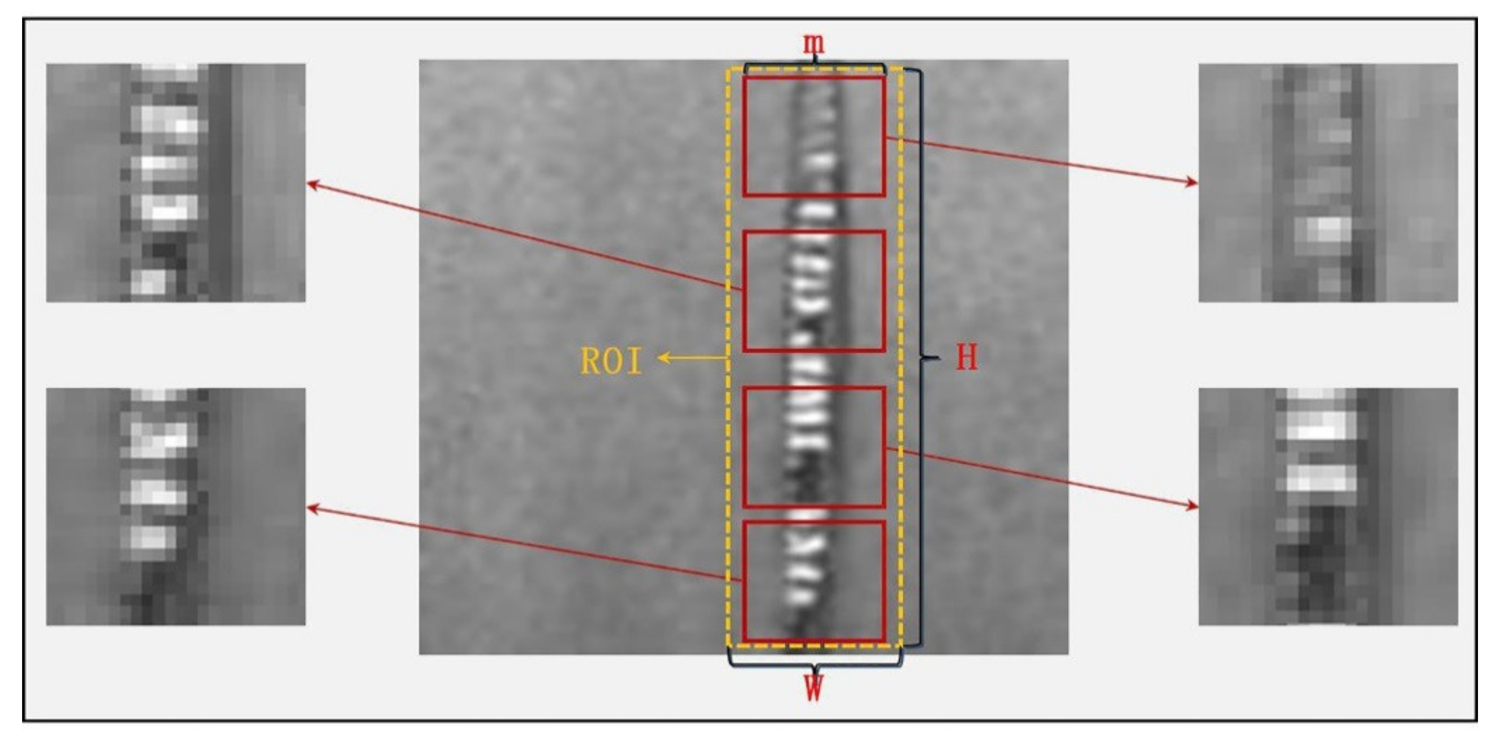
Based on the limitations of existing image data augmentation techniques, this paper proposed an industrial image data augmentation algorithm based on ROI region random cropping. Figure 11 is a strip steel surface image captured by CCD camera, and ROI region labeled with the approximate location of the defect. The rectangle side length of each side is W, H. The defect area is denoted as g. To ensure the defect area is larger than a quarter of the ROI region (25% ≦ area(g)), the formula can be defined as follows:
25 % a r e a ( g )   a r e a ( R O I ) a r e a ( g )   a r e a ( R O I )
This generates a square crop box in the ROI region randomly. Where the boxes’ side length is m, it is required that m at least be equal to or greater than 2/3 of the ROI rectangle’s minimum side length. The formula can be defined as follows:
2 3 [ min W , H ] m
Figure 11. Image data augmentation algorithm based on ROI region random crop.
Applsci 11 02606 g011
This algorithm can generate high-quality industrial images from original image datasets on the actual images demanded. It can not only solve the category imbalance problem using the data level approach method but also can be combined with traditional image data augmentation techniques to ease the problems of few samples datasets to a certain extent.
For the uneven difficulty samples (simple samples leading to loss function) problems, the key to solving them is the algorithm level approach method [35,36,37,38,39]. The industrial image data augmentation algorithm based on ROI region random crop in this paper can extract details of samples’ characteristics and enlarge images’ edge and other fine trivial details in the ROI region. This is a data level approach method to ease the uneven difficulty samples problem to a certain extent, and allow difficult samples to be identified by local details.

5. Strip Steel Surface Defect Recognition Deep Neural Network Based on Transfer Learning

5.1. Image Detection Problem on Low-Resolution and Few Samples

In traditional machine learning algorithms, a more complex model is more able to fit training data. However, a complex training model requires a large amount of data; if the training dataset is too small, the model will become over-fitted. This means the model fitting is perfect for the training dataset, but has poor generalization ability to testing data. This phenomenon is more obvious in deep learning neural networks [45]. Taking the ImageNet project as an example, it is a large image vision database for research, including more than 20,000 categories of images and more than 14 million manually annotated images. With the support of the ImageNet project’s database, deep learning develops rapidly.
According to image recognition contest experience of ImageNet, re-training an effective neural network convolution needs at least 1000 high-quality images of the same category. It can be seen in Figure 9 that the dataset in this paper is a typical few samples and imbalanced dataset. The dataset unable to enough to support deep learning network training. For this type of dataset, an improved VGG19 transfer learning network was proposed in this paper.

5.2. Transfer Learning Deep Neural Network Based on VGG19

The deep learning network requires a lot of high-quality annotated image data, but strip steel defects emerge randomly on the industrial production line. It takes a long time for strip steel production lines to collect enough defective samples, especially new strip steel production lines. To solve this problem, this paper chooses the VGG19 network [27] as the basic backbone and transfers its pre-trained parameters on ImageNet to our mixed image dataset. ImageNet dataset is mainly the data of life scenes (such as cats, bicycles, people), which has a big gap with the strip defect dataset in this paper. However, ImageNet dataset has a huge amount of data, and the VGG19 network model will not be overfitted on this dataset. Therefore, this paper fine-tune the VGG19 network pre-trained on ImageNet dataset to complete strip defect detection. With the help of transfer learning, our network achieved strip steel defect-recognition successfully.
A network trained with a transfer learning paradigm was designed to achieve automatic defect recognition. In the mixed dataset, we randomly selected 80% of the dataset to train the network classifier, and the remaining 20% of the dataset was used to test the network performance. The network’s input images were pre-processed by our improved gray-scale projection algorithm and ROI image augmentation algorithm. This is a strip steel defect dataset with full annotation and class balance. Model prediction accuracy and error are closely related. The mixed image dataset was pre-processed to create a new class balanced dataset; accuracy and categorical cross-entropy loss function are ideal indicators for evaluating the performance of various algorithms. In order to reflect the performance of the models, Formulas (3) and (4) were proposed.
Accuracy = Number   of   Correctly   Classified   Images Total   Number   of   Input   Images × 100 %
Loss ( P ,   Q )   =   i = 1 N P ( i ) log Q ( i )
where P (i) is the probability calculated after softmax activation, Q (i) is the prediction output of the model, and N is the number of categories.
The VGG19 network was designed as the basic backbone of our new network. The first 15 layers of the network were non-trainable frozen layers, while the four layers of the bottom network were used to conduct fine-tuning on the training dataset in the paper. Additionally, the loss function softmax cross-entropy classification was connected. Finally, matching with output classes, the strip steel defect-recognition transfer learning network based on VGG19 was construction. The initial learning rate was set as lr = 10−6, the attenuation rate was set as decay = 10−6, the attenuation momentum moment at 0.9, and the training step was 500 steps. The model was designed using Python 3.6 programming language, with Keras and TensorFlow libraries. The experimental equipment in this paper was a desktop personal computer with a I5-8500 processor, NVIDIA GTX 1050 graphics card, 32G RAM and hard disk capacity of 1T.
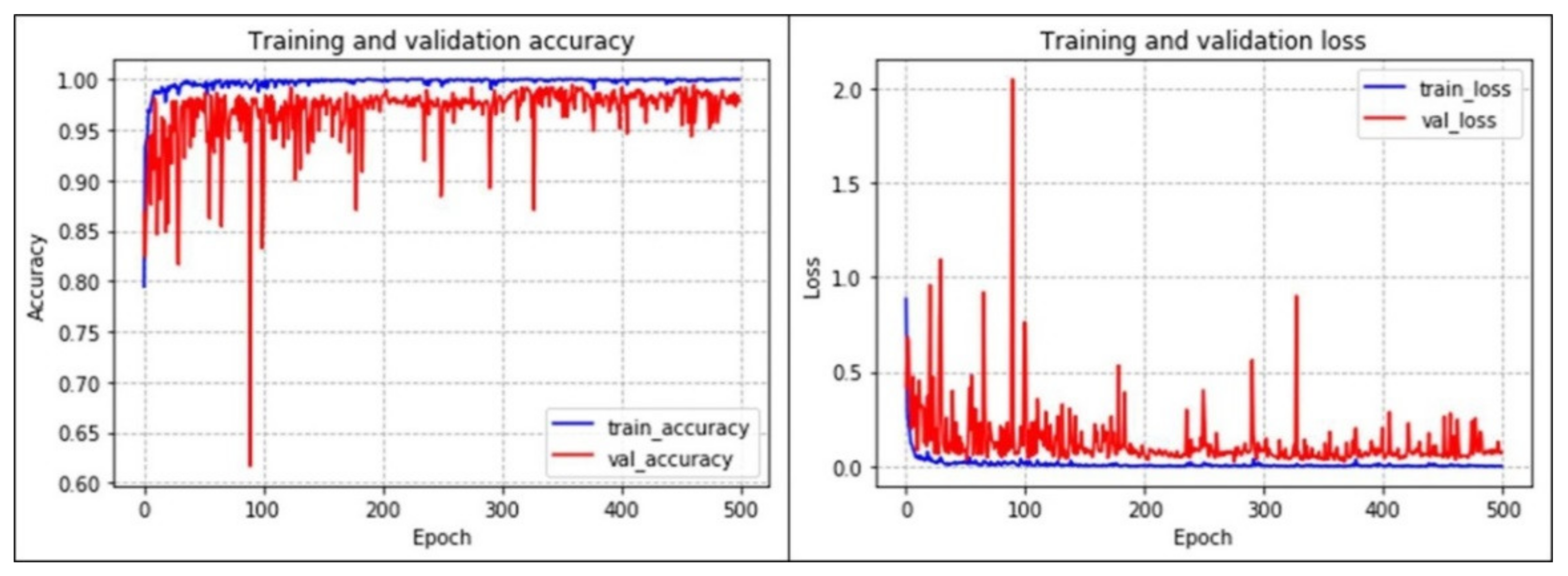
Figure 12 shows the accuracy and loss error of the network. The network has a poor convergence performance on the testing dataset. Checking the loss of error curve of the training process carefully, it was found that the verified loss of the dataset was quite turbulent in the early stage of training. In the medium term, there as occasional increases in loss. Although the loss converges after training, the unstable loss curve obviously has some unreasonable network design and network structure, needing further improvement.

5.3. A Transfer Learning Deep Neural Network Based on Improved VGG19

The current VGG19 network’s learning rate was a training step method based on the learning rate decay. Since the underlying textures of strip steel are relatively fine, in order to obtain detailed defect information, the network’s learning rate was set quite low. This resulted in slow convergence and falling to the local optimal value of the network, while the loss curve shocked greatly on the testing dataset, and achieved poor generalization.
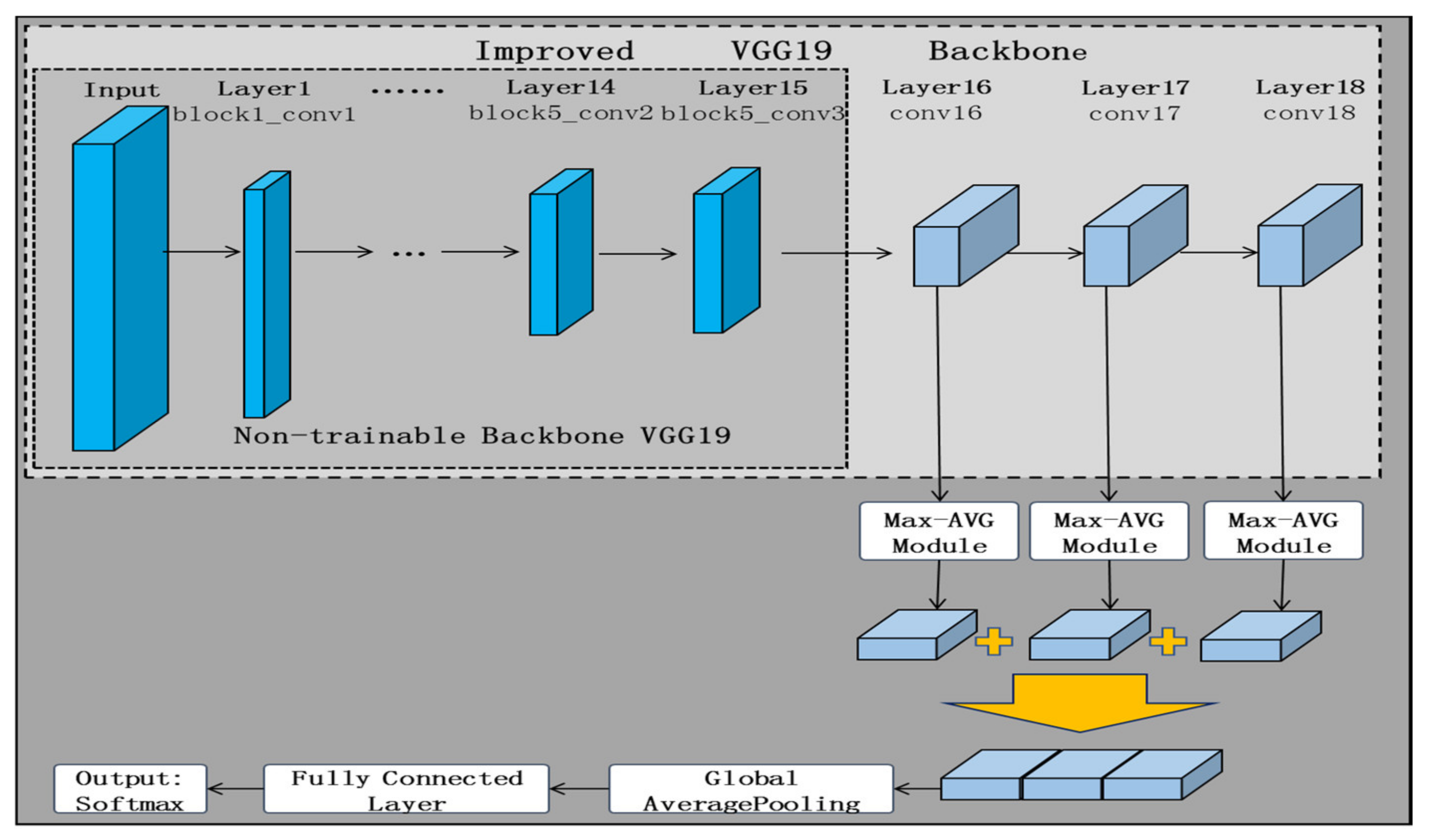
For the low learning rate problem, this paper proposed a hierarchical difference learning rate method. This means that underlying layers’ learning rates were set low, so that edges and other fine geometry features can be carefully learned and responded to, while the layers’ learning rates were set higher to ensure the network learned the images’ high-level features faster and to solve the problem of slow convergence on the network. In view of the above difficulties, this paper still used the VGG19 transfer learning network as a backbone in Section 5.2. The first 15 frozen layers are still non-trainable, but the remaining convolution layer and three full connection layers of the original network were discarded. These four network layers were replaced by three convolution network layers. Therefore, the improved VGG19 backbone neural network had 18 layers in total; the network layers set their learning rates as 10−6, 10−4 and 10−2 for different layer areas by the rule of 2:2:6.
By observing images of strip steel surface, we found whether the surface defect area had a higher brightness or a darker brightness than the defect-free area. In Section 3.4, the defect feature extraction algorithm proposed in this paper showed poor recognition of high brightness defects. Based on the above problems, a maximum and average feature extraction module was designed in this paper. As shown in Figure 13, this module has three branches, where the original features are processed in different convolutional layers, and finally connected by the concate layer.
Branch 1: The original features are sequentially passed through a convolution layer of size 1 × 1 and a convolution layer of size 2 × 2. This branch is not specially processed so that branch 1 can save the features in the original image as much as possible.
Branch 2: The original features are sequentially passed through a convolution layer of size 1 × 1 and an average pooling layer of size 2 × 2, and finally a ReLU activation layer is connected. Branch 2 uses the averaging pooling layer mainly to filter out the interference information in the original features.
Branch 3: The original features are sequentially passed through a convolution layer of size 1 × 1 and a maximum pooling layer of size 2 × 2, and finally a ReLU activation layer is connected. Branch 3 adopts the maximum pooling layer mainly to extract the features with higher brightness from the original features, so as to better find the defect area.
In order to allow the improved VGG19 backbone neural network to extract multi-level feature information, the 17th, 18th and 19th layers were connected with a maximum and average feature extraction module and a convolution layer, respectively. Then, the multi-level features extracted from the three branch layers were combined to connect a global pooling layer and a full connection layer. Finally, the network was connected to the softmax classifier. As shown in Figure 14, the improved transfer learning network was constructed.
In the optimization process of the network it is easy for it to drop into the local optimal problem. We referenced Author’s work [46], and from this the RAdam (Rectified Adam) optimizer was introduced to avoid the VGG19 network dropping into the local optimal. RAdam has the advantages of both Adam and SGD, which can not only ensure fast convergence speed but also avoid dropping into the local optimal, as the convergence result is insensitive to the network’s initial value learning rate. RAdam has a better performance than SGD in the case of a network having a large learning rate and limited training dataset.
Figure 15 shows that the convergence and accuracy of the network was greatly improved on the basic network. The model occasionally had a sudden increase in loss during the training period, but the verification function’s loss decreased and tended to converge as the training progressed. After the test, the final accuracy of the model converged to 97.8% and the generalization and robustness had been greatly improved, which had a certain practical value.
Figure 16 shows the comparison of the performance of the two algorithms, baseline VGG19 and improved VGG19, more intuitively, with the accuracy and loss curves of these two algorithms put into a unified ordinate system.
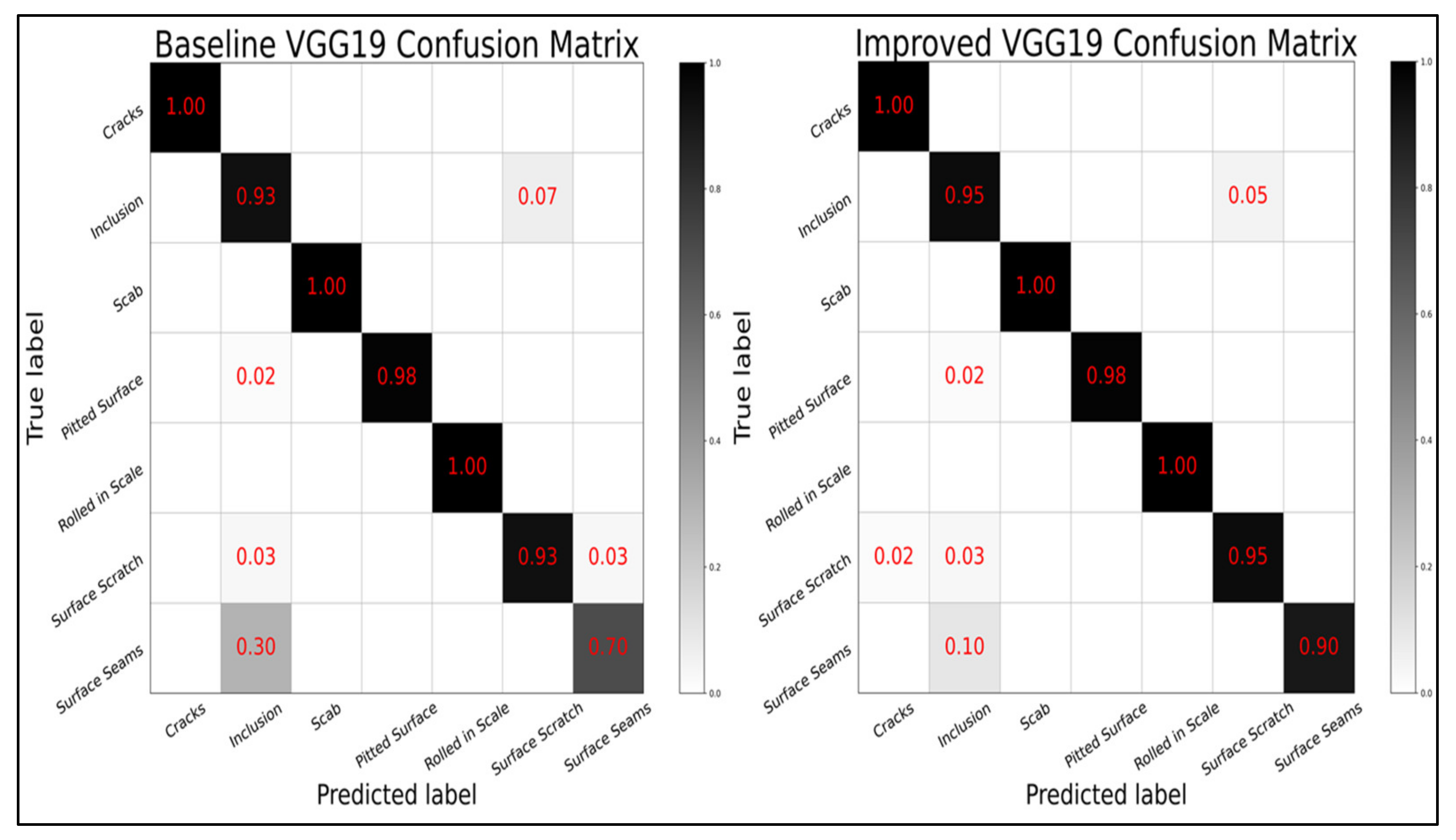
Figure 17 shows the baseline VGG19 and improved VGG19 network models’ confusion matrix on the test dataset. In order to be closer to actual production, the ROI region image augmentation algorithm in this paper was not augmented to achieve sample balance in categories on the testing dataset. It can be seen that both the baseline VGG19 and the improved VGG19 model can fully identify categories of cracks, scabs, and rolled in scales. These three types of defects have obvious features and are easy for the model to recognize. For the defect categories of inclusions, the baseline VGG19 misidentified four pieces of pictures and the improved VGG19 model misidentified three pieces of pictures. For the defect of pitted surfaces, both the baseline VGG19 and the improved VGG19 model misidentified one piece of picture. For the defect categories of surface scratch, the baseline VGG19 misidentified four pieces of pictures and the improved VGG19 model misidentified three pieces of pictures.
The improved VGG19 network performs slightly better than the baseline VGG19 in these six types of defects, but the improved VGG19 performs significantly better in the surface seams defects. However, the surface seams dataset has only 40 pieces of pictures and only 10 pieces of pictures for the testing dataset. Therefore, the accuracy of the baseline VGG19 and the improved VGG19 model on surface seams dataset are 70% and 90%, respectively. These indicators can be seen in the classification test report in Table 2.

6. Discussion

As can be seen from Table 3, traditional detection algorithms can achieve high detection accuracy with fewer images, but their real-time performance is poor. These algorithms include the HSVM-MC [15], HCGA [11], and CAE-SGAN [47]. For deep learning detection algorithms (such as M-Pooling CNN [17], Improved YOLO [19]), their detection accuracy increases with data volume and their real-time performance is better than that of the traditional algorithms. In this paper and references, “average detection time” refers to the sum of the time from data input to their models to get results. This time does not include the delay in image acquisition and data transmission between systems. This time is only a theoretical detection time. In the actual production line, the actual time is slightly larger than this value due to data transfer between different task modules.
Our network’s average detection time for a single image was 0.0183 s, and it can detect about 54 images per second. Considering that the speed of a steel rolling production line is 10–30 m/s and the view field of a single camera is 50–100 cm, it requires a detection speed of detection system to be 10–60 FPS. Compared with the M-pooling CNN algorithm and improved YOLO algorithm, our algorithm used the least amount of data. Its real-time performance was weaker than those two algorithms, but the detection speed of our network was 54.6 FPS, which means it meets the basic requirements of online real-time detection.
To further verify the performances of our algorithm in this paper, we tested and compared various algorithms on the Northeastern University (NEU) surface defect database. As can be seen from Table 4, a very deep network is not really required for the online real-time defect classification task; the detection accuracy, speed and complexity of the network need to be balanced.
Although the model in Author’s work [48] achieved an accuracy of 98.1% and a recognition speed of 476.2 FPS (2.1 ms), a NVIDIA GeForce GTX 1080Ti was used to train and test the neural network. Although the model is simple in structure and easy to build, the original data were pre-processed by the normalization Z-Score function. It is not an end-to-end model, and the time to pre-process the original data was much greater than the time for the network to recognize defects.
It is clear that a model with a certain complexity can not only achieve high accuracy and recognition speed, but also prevent the problem of non-convergence and over-fitting.
In order to improve the real-time performance of our network, the accuracy of network recognition could be improved by increasing the amount of training data, so as to further simplify the network structure to achieve higher accuracy and faster real-time detection (above 60 FPS).

7. Conclusions

The paper presents the processes of rapid screening surface, defect feature extraction, class balance, sample data augmentation, defect detection and classification. This is a set of processes required to complete strip steel defect detection. With these, we can meet the basic requirements of online real-time detection.
However, there are still some limitations in this paper. With continued production line developments, various kinds of new defect types will be created. When there is a similarity between a new defect form and a known defect form, the model will make a misjudgment, which will greatly reduce the accuracy of defect recognition. To address this problem, solution in this paper is continuing to collect new defect images to update the database and retrain the model offline. Regularly updating the model deployment to the production line will ensure the model is accurate on new types of defects.
In summary, this paper proposed An Improved VGG19 Transfer Learning Strip Steel Surface Defect Recognition Deep Neural Network Based on Few Samples and Imbalanced Datasets, which has a strong generalization and good convergence. It is a non-contact and non-destructive machine vision detection method that has the advantages of a high detection rate, strong real-time performance, and perfect anti-interference.
For the differences between the baseline VGG19 and the improved VGG19, we compared their confusion matrix, precision, recall, and F1-score of the two models in Figure 17 and Table 2. The improved VGG19 network performs slightly better than the baseline VGG19 in six types of defects, but the improved VGG19 performs significantly better in the surface seams defects. The experimental results show that the improved VGG19 network proposed in this paper has high practicability and reliability; it has a certain practical value for strip steel defects detection. In view of the limitations of research content, it is hoped that machine vision can be combined with various sensor technologies to achieve the comprehensive evaluation of multi-modal data fusion for defect detection and grading of strip steel, so as to improve the accuracy and real-time performance of this model, and allow it to better adapt to actual strip steel production in the future.

Author Contributions

X.W. conceived and drafted the original manuscript. X.Z. collected original data and computing. L.L. approved the final version of the paper and funding acquisition. All authors have read and agreed to the published version of the manuscript.

Funding

This research was funded by “The construction of professional CPS test and verification bed for the application of steel rolling process, grant number TC17085JH”.

Institutional Review Board Statement

Not applicable.

Informed Consent Statement

Not applicable.

Data Availability Statement

Publicly available datasets were analyzed in this study. This data can be found here: http://faculty.neu.edu.cn/yunhyan/NEU_surface_defect_database.html, accessed on 15 March 2021.

Acknowledgments

We would like to thank the Shanghai Key Laboratory of Intelligent Manufacturing & Robotics and all members of the CIMS laboratory for their support.

Conflicts of Interest

The authors declare no conflict of interest.

Abbreviations

A-Fast-RCNNAdversarial Fast Region-based Convolutional Neural Network
BMPBitmap
CCDCharge Coupled Device
CNNConvolution Neural Network
CAE-SGANConvolutional Autoencoder Extract and Semi-supervised
Generative Adversarial Networks
DNNDeep Neural Network
FCNFully Convolutional Network
FPSFrames Per Second
GANsGenerative Adversarial Networks
GHMGradient Harmonizing Mechanis
HSVM-MCMulti-label Classifier with Hyper-sphere Support
Vector Machine
HCGAHybrid Chromosome Genetic Algorithm
MFNMultilevel Feature Fusion Network
NEUNortheastern University
M-Pooling CNNMax-Pooling Convolution Neural Network
OHEMOnline Hard Example Mining
PLCNNConvolution Neural Network based on Pseudo-Label
ROIRegion of Interest
ResNetResidual Network
RAdamRectified Adam
S-OHEMStratified Online Hard Example Mining
SVMSupport Vector Machines
SGDStochastic Gradient Descent
VGGVery Deep Convolutional Networks designed by Visual
Geometry Group
YOLOYou Only Look Once

References

  1. Wu, P.; Lu, T.; Wang, Y. Nondestructive testing technique for strip surface defects and its applications. Nondestruct. Test. 2000, 22, 312–315. [Google Scholar]
  2. Tian, S.; Xu, K. An Algorithm for Surface Defect Identification of Steel Plates Based on Genetic Algorithm and Extreme Learning Machine. Metals 2017, 7, 311. [Google Scholar] [CrossRef]
  3. Srinivasan, K.; Dastoor, P.H.; Radhakrishnaiah, P.; Jayaraman, S. FDAS: A Knowledge-based Framework for Analysis of Defects in Woven Textile Structures. J. Text. Inst. 1992, 83, 431–448. [Google Scholar] [CrossRef]
  4. Yin, X.; Yu, X.; Sohn, K.; Liu, X.; Chandraker, M. Feature Transfer Learning for Face Recognition with Under-Represented Data. In Proceedings of the 2019 IEEE Conference on Computer Vision and Pattern Recognition (CVPR), Long Beach, CA, USA, 15–20 June 2019; pp. 5697–5706. [Google Scholar]
  5. Cui, Y.; Jia, M.; Lin, T.Y.; Song, Y.; Belongie, S. Class-Balanced Loss Based on Effective Number of Samples. In Proceedings of the 2019 IEEE Conference on Computer Vision and Pattern Recognition (CVPR), Long Beach, CA, USA, 15–20 June 2019; pp. 9260–9269. [Google Scholar]
  6. Fang, X.; Luo, Q.; Zhou, B.; Li, C.; Tian, L. Research Progress of Automated Visual Surface Defect Detection for Industrial Metal Planar Materials. Sensors 2020, 20, 5136. [Google Scholar] [CrossRef] [PubMed]
  7. Shi, T.; Kong, J.; Wang, X.; Liu, Z.; Zheng, G. Improved sobel algorithm for defect detection of rail surfaces with enhanced efficiency and accuracy. J. Cent. South. Univ. 2016, 23, 2867–2875. [Google Scholar] [CrossRef]
  8. Ma, Y.; Li, Q.; Zhou, Y.; He, F.; Xi, S. A surface defects inspection method based on multidirectional gray-level fluctuation. Int. J. Adv. Robot. Syst. 2017, 14, 1–17. [Google Scholar] [CrossRef] [Green Version]
  9. Ojala, T.; Pietikainen, M.; Harwood, D. A comparative study of texture measures with classification based on feature distributions. Pattern Recognit. 1996, 29, 51–59. [Google Scholar] [CrossRef]
  10. Jeon, Y.; Yun, J.; Choi, D.; Kim, S.W. Defect detection algorithm for corner cracks in steel billet using discrete wavelet transform. In Proceedings of the ICROS-SICE International Joint Conference, Fukuoka, Japan, 18–21 August 2009; pp. 2769–2773. [Google Scholar]
  11. Hu, H.; Liu, Y.; Liu, M.; Nie, L. Surface Defect Classification in Large-scale Strip Steel Image Collection via Hybrid Chromosome Genetic Algorithm. Neurocomputing 2016, 181, 86–95. [Google Scholar] [CrossRef]
  12. Yazdchi, M.; Yazdi, M.; Mahyari, A.G. Steel surface defect detection using texture segmentation based on multifractal dimension. In Proceedings of the International Conference on Digital Image Processing (ICDIP), Bangkok, Thailand, 7–9 March 2009; pp. 346–350. [Google Scholar]
  13. Mandriota, C.; Nitti, M.; Ancona, N.; Stella, E.; Distante, A. Filter-based feature selection for rail defect detection. Mach. Vis. Appl. 2004, 15, 179–185. [Google Scholar] [CrossRef]
  14. Tang, B. Steel Surface Defect Recognition Based on Support Vector Machine and Image Processing. China Mech. Eng. 2011, 22, 1402–1405. [Google Scholar]
  15. Chu, M.; Zhao, J.; Gong, R.; Liu, L. Steel surface defects recognition based on multi-label classifier with hyper-sphere support vector machine. In Proceedings of the Control and Decision Conference (CCDC), Chongqing, China, 28–30 May 2017; pp. 3276–3281. [Google Scholar]
  16. Kwon, B.K.; Won, J.S.; Kang, D.J. Fast defect detection for various types of surfaces using random forest with VOV features. Int. J. Precis. Eng. Manuf. 2015, 16, 965–970. [Google Scholar] [CrossRef]
  17. Masci, J.; Meier, U.; Ciresan, D.; Schmidhuber, J.; Fricout, G. Steel defect classification with Max-Pooling Convolutional Neural Networks. In Proceedings of the 2012 International Joint Conference on Neural Networks (IJCNN), Brisbane, QLD, Australia, 10–15 June 2012; pp. 1–6. [Google Scholar]
  18. Gao, Y.; Gao, L.; Li, X.; Yan, X. A semi-supervised convolutional neural network-based method for steel surface defect recognition. Robot. Comput. Integr. Manuf. 2020, 61, 101825. [Google Scholar] [CrossRef]
  19. Li, J.; Su, Z.; Geng, J.; Yin, Y. Real-time Detection of Steel Strip Surface Defects Based on Improved YOLO Detection Network. IFAC-Pap. 2018, 51, 76–81. [Google Scholar] [CrossRef]
  20. Geirhos, R.; Rubisch, P.; Michaelis, C.; Bethge, M.; Wichmann, F.A.; Brendel, W. ImageNet-trained CNNs are biased towards texture; increasing shape bias improves accuracy and robustness. In Proceedings of the International Conference on Learning Representations (ICLR 2019), New Orleans, LA, USA, 6–9 May 2019. [Google Scholar]
  21. Kim, S.; Kim, W.; Noh, Y.K.; Park, F.C. Transfer learning for automated optical inspection. In Proceedings of the International Joint Conference on Neural Networks, Anchorage, AK, USA, 14–19 May 2017; pp. 2517–2524. [Google Scholar]
  22. He, Y.; Song, K.; Meng, Q.; Yan, Y. An End-to-End Steel Surface Defect Detection Approach via Fusing Multiple Hierarchical Features. IEEE Trans. Instrum. Meas. 2020, 69, 1493–1504. [Google Scholar] [CrossRef]
  23. Dung, C.V.; Anh, L.D. Autonomous concrete crack detection using deep fully convolutional neural network. Autom. Constr. 2018, 99, 52–58. [Google Scholar] [CrossRef]
  24. Han, T.; Liu, C.; Yang, W.; Jiang, D. Deep transfer network with joint distribution adaptation: A new intelligent fault diagnosis framework for industry application. ISA Trans. 2020, 97, 269–281. [Google Scholar] [CrossRef] [Green Version]
  25. Mun, S.; Shin, M.; Shon, S.; Kim, W.; Han, D.K.; Ko, H. DNN Transfer learning based non-linear feature extraction for acoustic event classification. IEICE Trans. Inf. Syst. 2017, 100, 2249–2252. [Google Scholar] [CrossRef] [Green Version]
  26. Qureshi, A.S.; Khan, A.; Zameer, A.; Usman, A. Wind power prediction using deep neural network based meta regression and transfer learning. Appl. Soft Comput. 2017, 58, 742–755. [Google Scholar] [CrossRef]
  27. Simonyan, K.; Zisserman, A. Very deep convolutional networks for large-scale image recognition. In Proceedings of the 3rd International Conference on Learning Representations (ICLR 2015), San Diego, CA, USA, 7–9 May 2015. [Google Scholar]
  28. Zhang, J.; Mani, I. KNN Approach to Unbalanced Data Distributions: A Case Study Involving Information Extraction. In Proceedings of the ICML’2003 Workshop on Learning from Imbalanced Datasets, Washington, DC, USA, 21 August 2003. [Google Scholar]
  29. He, H.; Bai, Y.; Garcia, E.A.; Li, S. ADASYN: Adaptive Synthetic Sampling Approach for Imbalanced Learning. In Proceedings of the 2008 IEEE International Joint Conference on Neural Networks (IEEE World Congress on Computational Intelligence), Hong Kong, China, 1–8 June 2008; pp. 1322–1328. [Google Scholar]
  30. Batista, G.E.; Prati, R.C.; Monard, M.C. A study of the behavior of several methods for balancing machine learning training data. ACM Sigkdd Explor. Newsl. 2004, 6, 20. [Google Scholar] [CrossRef]
  31. Elkan, C. The foundations of cost-sensitive learning. In Proceedings of the Seventeenth International Conference on Artificial Intelligence, Seattle, USA, 4–10 August 2001; pp. 973–978. [Google Scholar]
  32. Liu, X.Y.; Zhou, Z.H. The Influence of Class Imbalance on Cost-Sensitive Learning: An Empirical Study. In Proceedings of the 6th IEEE International Conference on Data Mining (ICDM 2006), Hong Kong, China, 18–22 December 2006. [Google Scholar]
  33. Wang, S.; Yao, X. Diversity Analysis on Imbalanced Data Sets by Using Ensemble Models. In Proceedings of the IEEE Symposium on Computational Intelligence and Data Mining, CIDM 2009, part of the IEEE Symposium Series on Computational Intelligence 2009, Nashville, TN, USA, 30 March–2 April 2009. [Google Scholar]
  34. Liu, X.Y.; Wu, J.; Zhou, Z.H. Exploratory Undersampling for Class-Imbalance Learning. IEEE Trans. Cybern. 2009, 39, 539–550. [Google Scholar]
  35. Shrivastava, A.; Gupta, A.; Girshick, R. Training Region-Based Object Detectors with Online Hard Example Mining. In Proceedings of the 2016 IEEE Conference on Computer Vision and Pattern Recognition (CVPR), Las Vegas, NV, USA, 27–30 June 2016; pp. 761–769. [Google Scholar]
  36. Li, M.; Zhang, Z.; Yu, H.; Chen, X.; Li, D. S-OHEM: Stratified Online Hard Example Mining for Object Detection. In Proceedings of the Chinese Conference on Computer Vision, Tianjin, China, 11–14 October 2017. [Google Scholar]
  37. Wang, X.; Shrivastava, A.; Gupta, A. A-Fast-RCNN: Hard Positive Generation via Adversary for Object Detection. In Proceedings of the 2017 IEEE Conference on Computer Vision and Pattern Recognition (CVPR), Honolulu, HI, USA, 21–26 July 2017; pp. 3039–3048. [Google Scholar]
  38. Lin, T.Y.; Goyal, P.; Girshick, R.; He, K.; Dollár, P. Focal Loss for Dense Object Detection. In Proceedings of the IEEE International Conference on Computer Vision, Venice, Italy, 22–29 October 2017; pp. 2999–3007. [Google Scholar]
  39. Li, B.; Liu, Y.; Wang, X. Gradient Harmonized Single-stage Detector. In Proceedings of the Thirty-Third AAAI Conference on Artificial Intelligence (AAAI2019), Hilton Hawaiian Village, Honolulu, HI, USA, 27 January–1 February 2019. [Google Scholar]
  40. NEU Surface Defect Database. Available online: http://faculty.neu.edu.cn/yunhyan/NEU_surface_defect_database.html (accessed on 8 January 2021).
  41. Springer Nature Editorial. More accountability for big-data algorithms. Nature 2016, 537, 449. [Google Scholar] [CrossRef] [PubMed] [Green Version]
  42. Ghiasi, G.; Lin, T.Y.; Le, Q.V. DropBlock: A regularization method for convolutional networks. In Proceedings of the 32nd Conference on Neural Information Processing Systems (NIPS), Montreal, QC, Canada, 2–8 December 2018. [Google Scholar]
  43. Singh, K.K.; Lee, Y.J. Hide-and-Seek: Forcing a Network to be Meticulous for Weakly-supervised Object and Action Localization. In Proceedings of the 16th IEEE International Conference on Computer Vision (ICCV), Venice, Italy, 22–29 October 2017. [Google Scholar]
  44. Zhao, Z.; Li, B.; Dong, R. A Surface Defect Detection Method Based on Positive Samples. In Proceedings of the 5th Pacific Rim International Conference on Artificial Intelligence (PRICAI), Nanjing, China, 28–31 August 2018. [Google Scholar]
  45. Sun, C.; Shrivastava, A.; Singh, S.; Gupta, A. Revisiting Unreasonable Effectiveness of Data in Deep Learning Era. In Proceedings of the 16th IEEE International Conference on Computer Vision (ICCV), Venice, Italy, 22–29 October 2017. [Google Scholar]
  46. Liu, L.; Jiang, H.; He, P.; Chen, W.; Liu, X.; Gao, J.; Han, J. On the Variance of the Adaptive Learning Rate and Beyond. In Proceedings of the International Conference on Learning Representations (ICLR 2020), Addis Ababa, Ethiopia, 26–30 April 2020. [Google Scholar]
  47. Di, H.; Ke, X.; Peng, Z.; Dongdong, Z. Surface defect classification of steels with a new semi-supervised learning method. Opt. Lasers Eng. 2019, 117, 40–48. [Google Scholar] [CrossRef]
  48. Kostenetskiy, P.; Alkapov, R.; Vetoshkin, N.; Chulkevich, R.; Napolskikh, I.; Poponin, O. Real-time system for automatic cold strip surface defect detection. FME Trans. 2019, 47, 765–774. [Google Scholar] [CrossRef] [Green Version]
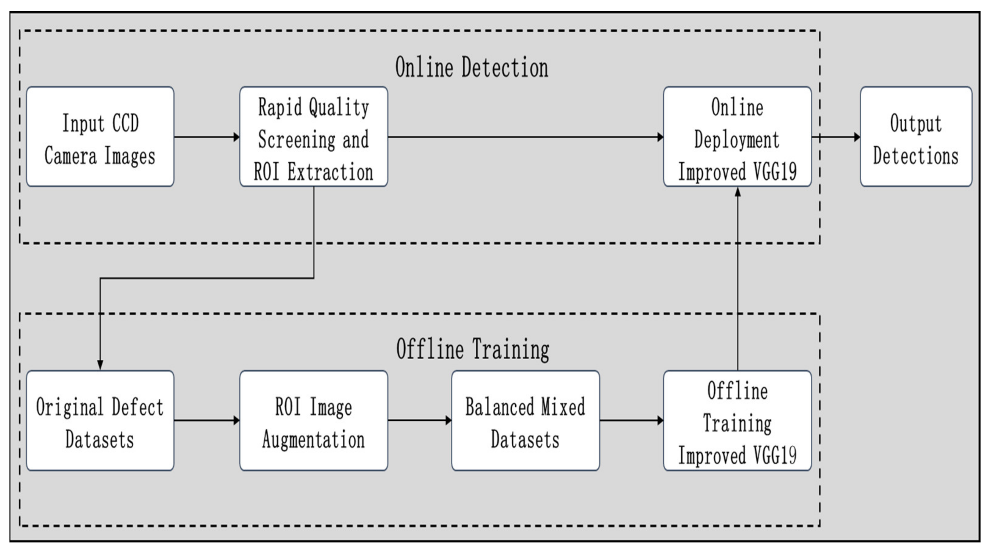
Figure 1. Overview of the strip steel defect detection method.
Applsci 11 02606 g001
Figure 2. Image of the strip steel edge region and background region.
Applsci 11 02606 g002
Figure 3. Image of a strip steel defect acquisition region.
Applsci 11 02606 g003
Figure 4. Strip steel defect acquisition region processed by the Canny edge detection operator.
Applsci 11 02606 g004
Figure 5. Column detection results of the steel strip.
Applsci 11 02606 g005
Figure 6. Detection results of the steel strip.
Applsci 11 02606 g006
Figure 7. Detection results of a longitudinal flaw image.
Applsci 11 02606 g007
Figure 8. The contrast of our algorithm’s performance on defect-free and defect surfaces.
Applsci 11 02606 g008
Figure 9. Strip steel defect categories.
Applsci 11 02606 g009
Figure 10. Process of strip steel surface rapidly quality screening and defect feature extraction.
Applsci 11 02606 g010
Figure 12. The accuracy and loss error of the baseline VGG19 network.
Applsci 11 02606 g012
Figure 13. Maximum and Average feature extraction module.
Applsci 11 02606 g013
Figure 14. Improved VGG19 with feature extraction modules.
Applsci 11 02606 g014
Figure 15. The accuracy and loss error of improved VGG19 network.
Applsci 11 02606 g015
Figure 16. The accuracy and loss error differences between the baseline VGG19 and improved VGG19 network.
Applsci 11 02606 g016
Figure 17. Confusion matrix of the test dataset.
Applsci 11 02606 g017
Table 1. Testing of Our Defect Feature Extraction Algorithm.
Samples24024024024024024040
Defectscracksinclusionsscabpitted surfacerolled in scalesurface scratchsurface seams
Accurate83.8%0.83%2.5%1.7%1.3%87.5%90.0%
Table 2. Report on the test dataset.
TargetsPrecisionRecallf1-ScoreSamples
Defects
Baseline VGG19 Network
Cracks1.00001.00001.00060
Inclusion0.90320.93330.918060
Scab1.00001.00001.000060
Pitted Surface1.00000.98330.991660
Rolled in Scale1.00001.00001.000060
Surface Scratch0.93330.93330.933360
Surface Seams0.77780.70000.736810
Weighted Avg0.96750.96760.9674370
Improved VGG19 Network
Cracks0.98361.00000.991760
Inclusion0.9344 0.95000.942160
Scab1.00001.00001.000060
Pitted Surface1.00000.98330.991660
Rolled in Scale1.00001.00001.000060
Surface Scratch0.95000.95000.950060
Surface Seams 1.00000.90000.947410
Weighted Avg0.97860.97840.9784370
Table 3. Performance comparison between traditional algorithms and DNN algorithms.
AlgorithmTaskAccuracyAverage Detection per ImageSamples
M-Pooling CNN [17]
Masci et al., 2012
DNN
Classification
93.03%0.0062 s
161.3 FPS
2927
HCGA [11]
Hu et al., 2015
Traditional
Classification
95.04%0.158 s
6.3 FPS
351
HSVM-MC [15]
(Chu et al., 2017)
Traditional Classification95.18%1.1044 s
0.9 FPS
900
Improved YOLO [19]
Jiangyun LI et al., 2018
DNN
Classification and location
97.55%0.012 s
83.3 FPS
4655
CAE-SGAN [47]
Di HE et al., 2019
Traditional
Classification
98.20%unknown10,800
OursDNN
Classification
97.75%0.0183 s
54.6 FPS
1850
Table 4. DNN Algorithms tested on NEU database.
AlgorithmAccuracyTime per Image
M-Pooling CNN [17]
Masci et al., 2012
93.37%0.007s
142.9FPS
CNN [48]
Kostenetskiy, P. et al., 2019
98.10%0.0021 s
476.2 FPS
PLCNN [18]
Yiping GAO et al., 2020
94.74%0.00865 s
115.6 FPS
ResNet50+MFN [22]
ResNet34+MFN
Yu HE et al., 2020
99.70%
99.20%
0.165 s/6.1 FPS
0.115 s/8.7 FPS
Ours97.62%0.0192 s/52.1 FPS
Publisher’s Note: MDPI stays neutral with regard to jurisdictional claims in published maps and institutional affiliations.