A Green’s Function for Acoustic Problems in Pekeris Waveguide Using a Rigorous Image Source Method

Abstract

The Green’s function (GF) directly eases the efficient computation for acoustic radiation problems in shallow water with the use of the Helmholtz integral equation. The difficulty in solving the GF in shallow water lies in the need to consider the boundary effects. In this paper, a rigorous theoretical model of interactions between the spherical wave and the liquid boundary is established by Fourier transform. The accurate and adaptive GF for the acoustic problems in the Pekeris waveguide with lossy seabed is derived, which is based on the image source method (ISM) and wave acoustics. First, the spherical wave is decomposed into plane waves in different incident angles. Second, each plane wave is multiplied by the corresponding reflection coefficient to obtain the reflected sound field, and the field is superposed to obtain the reflected sound field of the spherical wave. Then, the sound field of all image sources and the physical source are summed to obtain the GF in the Pekeris waveguide. The results computed by this method are compared with the standard wavenumber integration method, which verifies the accuracy of the GF for the near- and far-field acoustic problems. The influence of seabed attenuation on modal interference patterns is analyzed.

1. Introduction

The Green’s function (GF) is the fundamental element in the acoustic calculation, which describes the sound field generated by a point source under certain boundary conditions or initial conditions, that is, the acoustic transfer relationship between the vibration source and the receiver is established. Therefore, the GF is widely used in the acoustic computational method, such as the Helmholtz integral method, which is generally a concise formulation of the partial differential equation for acoustic problems by using the Gaussian theory and automatically meeting the boundary conditions, the radiated sound field in different fluid environments (infinity field, half space, closed space, etc.) can be investigated efficiently by adjusting the GF of the Helmholtz integral method [1,2,3]. Additionally, the GF provides us with a lot of convenience of an acoustic problem where we can not only inverse the vibration characteristics of the source through the identified acoustic characteristics but can also easily calculate the pressure level at any point according to the configured radiator in the corresponding fluid [4]. Due to the GF having these advantages in acoustic computation, it is very significant for acoustic holography [5,6,7], beamforming [8], acoustic radiation and scattering [9,10,11], acoustic measurement [12], etc. By introducing the GF into the Helmholtz integral equation, acoustic calculations become simpler and more flexible. In the equation, boundary conditions on the surface of the source, such as the sound pressure (Dirichlet condition), the normal velocity (Neumann condition), and the boundary normal conductance (Robin condition), can be selectively given in the integral equation to match the elastic radiator for the acoustic radiation calculation [10], and a suitable GF can be chosen to establish the transfer relationship between the source on the structure surface and the sound field in the fluid environment. Thus, we can solve the radiated sound field or invert the vibration characteristics of the radiator via the scheme of combining the Helmholtz integral equation and the GF. Subsequently, computational methods such as boundary elements [13], equivalent sources [14], and hydroelasticity theory [15] have been extended to promote further developments in the fields of acoustic cloaking design, near-field acoustic field measurements, and target identification for underwater vehicles. However, when the integral method is utilized for the structural radiation in shallow water, the universal acoustic problems of the near and far field are inevitable. Consequently, the GF must be adjusted and adapt to such problems [16].

Different from the GF in infinity field or half space, the solution of the GF in shallow water involves different mathematical treatment and the corresponding applicable conditions. Physically, the GF in shallow water is the solution to the inhomogeneous Helmholtz equation for a point source, which satisfies the sound conditions of the upper and lower boundaries, which leads to the fact that the difficulty in deriving the GF in shallow water lies in establishing the interaction between the sound field and the boundaries, especially for seabeds with different types. Currently, the most prominent models for solving the GF in shallow water are the ray method [17], the normal mode (NM) method [18], the wavenumber integration (WI) method [19], and the parabolic equation (PE) method [20]. The theoretical foundation of all sound propagation models is the acoustic wave equation; it is only that the mathematical processing strategies used for nonhomogeneous wave equations are different, in addition to the form of the solution [21]. Therefore, each model has the applicable conditions that make it suitable for a practical problem.

To meet the requirements of studying the structural acoustic radiations in shallow water, in which the near- and far-field problem will be involved, a common strategy is to apply a combination of the near- and far-field GFs to ensure high computational efficiency and accuracy (e.g., the image source method (ISM) and the NM for the far- and near-field sound fields, respectively) [15,16]. However, there are some limitations to such a strategy. First, it will involve a distance connection problem of the near and far fields, which is inconvenient to execute in the calculation program. Additionally, the near-field ISM involves the problem of the difference between the symmetry of the incident spherical wave and the form of the fluid–fluid interface. The classical ISM, in which a process that uses the incident spherical wave multiplied directly by the constant reflection coefficient of the plane wave to represent the reflected sound field is feasible for an ideal seabed since the reflection coefficient is always constant (i.e., 1) at any angle, where each order of plane wave in a spherical wave multiplied by a constant is equal to a spherical wave multiplied directly by a constant. However, for the liquid seabed, for example, the Pekeris waveguide, the reflection coefficient of a plane wave at the liquid–liquid interface is not always constant, and when there is sound absorption in the seabed medium, there can be no total reflection. It is inaccurate to represent the reflected sound field by the spherical wave directly multiplied by a certain reflection coefficient. Therefore, the strategy of using a combination of the ISM and NM cannot accurately solve the far- and near-field acoustic problem, and a more adaptable GF needs to be explored.

In this paper, a rigorous ISM model of the interaction between the spherical wave and the plane interface on the liquid–liquid boundary is established by combining classical ISM with the wave acoustics, an accurate GF is derived for the near and far fields in the Pekeris waveguide, and the sound attenuation in a homogeneous liquid seabed is introduced. This theoretical model mainly consists of three parts. First, the spherical wave of a point source is decomposed into plane waves in different directions based on the Fourier transform. Then, we need to make the symmetry of the sound field waves unified with the form of the plane interface, as we are more familiar with the theory of reflection and transmission of plane waves. Thus, it is necessary to convert the spherical coordinates to Cartesian coordinates, then each plane wave is multiplied by the corresponding reflection coefficient to obtain the reflected sound field. Finally, all of the plane wave components of the reflected sound field are superimposed to obtain the spherical wave reflected by the liquid–liquid interface. The results calculated by this rigorous ISM are compared with the standard WI to verify the accuracy for the near- and far-field acoustic problem in the Pekeris waveguide.

2. Theoretical Model of the Rigorous ISM

The theoretical foundation of the classical ISM for deriving the GF in the Pekeris waveguide is ray acoustics, where the sound field at any field point can be expressed as a superposition summation of the direct wave radiated by the sound source and the sound field reflected by the fluid–fluid interface [22]. As shown in Figure 1a, the point source emits sound waves represented by the radiation rays, and then each ray follows the Snell theorem of reflection and transmission on the upper and lower interfaces (i.e., each ray is multiplied by the reflection coefficient of the corresponding incident angle, and the reflected sound field can be obtained at the certain field point, where the effects of the upper and lower boundaries on the physical source are considered by the image sources).

However, the traditional ISM is generally applied when the distance between the source and the receiver to the field is much larger than the wavelength (or far field), and the reflection problem of spherical waves on the interface can be approximated by the ISM. However, when the distance is comparable to the wavelength (i.e., the near field), the results of the traditional ISM have some deviations from the practical sound field, and then it is necessary to strictly observe the wave acoustics method to establish the interaction mechanism of the near-field spherical wave and the interface. As shown in Figure 1b, when the spherical wave radiated from the point source interacts with the liquid–liquid interface, the spherical wave needs to be decomposed into plane waves in different directions, and then the reflection theory of plane waves on the interface is used to obtain the reflected sound field of plane waves. Finally, these reflected sound fields are superimposed to derive the reflected sound field of the spherical wave on the plane liquid–liquid interface; these describe the rigorous ISM.

The traditional ISM of the propagation model is based on the ray theory, and the upper and lower boundaries in the homogeneous waveguide are considered by the image sources. Figure 1a shows a schematic diagram of the contributions from the physical source and the first three image sources; the remaining terms are obtained by successive imaging of these sources to yield the ray expansion for the total field [23]

$$\begin{array}{c}G(r,z)={\left(V_1{V}_2({\vartheta }_i)\right)}^m{\displaystyle \sum _{m=0}^{\infty }\left[\frac{e^{j{k}_a{R}_{m1}}}{R_{m1}}+\right.}{V}_2({\vartheta }_i)\frac{e^{j{k}_a{R}_{m2}}}{R_{m2}}+\\ \begin{array}{c}\left.V_1\frac{e^{j{k}_a{R}_{m3}}}{R_{m3}}+V_1{V}_2({\vartheta }_i)\frac{e^{j{k}_a{R}_{m4}}}{R_{m4}}\right]\end{array},\end{array}$$

(1)

where $V_1$ and $V_2$ are the reflection coefficients of the plane wave for upper and lower boundaries, respectively. It should be noted that $V_1=-1$ for the pressure-release surface, however, the bottom of the Pekeris waveguide is not an ideal rigid surface; the reflection coefficient $V_2$ does not remain constant but relates to the angle ${\vartheta }_i$, which is the incident angle of each term plane wave decomposed by the spherical wave on the seabed surface. $k_a$ is the sound wavenumber in the water, $R_{mn}=\sqrt{r^2+z_{mn}^2}$ and m is the number of mirrored sources, and the value is$m=0,1,2,3\dots ,\infty$, $n=1,2,3,4$, $z_{m1}=2Hm+z-z_s$, $z_{m2}=2Hm+z+z_s$, $z_{m3}=2H\left(m+1\right)-z-z_s$, $z_{m4}=2H\left(m+1\right)-z+z_s$. Generally, when m reaches tens of terms, the total sound field will quickly stabilize at a certain value.

Equation (1) is fulfilled by the Helmholtz wave equation because it is composed of multiple spherical waves, each of which satisfies the equation. Different from the processing method in ideal shallow water conditions with a rigid seabed (i.e., the $V_2$ is always 1), the reflection coefficient $V_2$ in the Pekeris waveguide depends on the incident angle and incident waveform (i.e., plane wave), and it is more similar to the reflection coefficient of the plane wave in the theoretical calculation. However, the sound field in Equation (1) is the sound superposition of spherical waves reflected by physical source and the image sources—it is essential to make the waveform and reflection coefficient consistent. In this rigorous ISM, the solution to this problem requires the decomposition of spherical waves into plane waves with various angles.

In the plane at z = 0, the sound field of a spherical wave can be expanded into a double Fourier integral with x and y [24], as follows:

$$\frac{e^{ik\mathrm{r}}}{\mathrm{r}}={\displaystyle \underset{-}{\overset{+}{\int }}{\displaystyle \underset{\infty }{\overset{\infty }{\int }}A(k_x,k_y)}}{e}^{i(k_{x}x+k_{y}y)}d{k}_{x}d{k}_y,$$

(2)

where r is the distance vector from the point source to the receiver, i is the imaginary part of the complex number, and the integral variables $k_x$ and $k_y$ are the vector projections of the wavenumber k in the direction of the x and y axes, respectively, and the spectral density of the wave, which is obtained by the inverse Fourier transform, as follows:

$$A(k_x,k_y)=\frac{1}{{(2\pi )}^2}{\displaystyle \underset{-}{\overset{+}{\int }}{\displaystyle \underset{\infty }{\overset{\infty }{\int }}\frac{e^{ikr}}{r}{e}^{-i(k_{x}x+k_{y}y)}d{k}_{x}d{k}_y}},$$

(3)

To obtain the value of $\left.A(k_x,k_y\right)$, we now establish the transformation between polar and Cartesian coordinates such that

$$x=r\cos \psi , y=r\sin \psi ,dxdy=rdrd\psi ,$$

(4)

$$k_x=l\cos \phi ,k_y=l\sin \phi ,l=\sqrt{k_x^2+k_y^2},$$

(5)

where l is the projection of the wave vector k on the xoy plane.

By substituting Equation (4) and Equation (5) into Equation (3), we find

$$A(k_x,k_y)=\frac{1}{{(2\pi )}^2}{\displaystyle {\int }_0^{2\pi }d\psi {\displaystyle {\int }_0^{\infty }{e}^{ir\left[k-l\cos (\phi -\psi )\right]}dr}}$$

(6)

The integral over r is elementary. Moreover, if we assume that there is some absorption in the medium, no matter how small (i.e., that k has a positive imaginary part), then the substitution of the upper limit yields zero, and finally, $\left.A(k_x,k_y\right)$is solved by integration operations and can be expressed as follows:

$$\begin{array}{l}A(k_x,k_y)=\frac{i}{{(2\pi )}^2}{\displaystyle {\int }_0^{2\pi }\frac{1}{k-l\cos (\phi -\psi )}d\psi }\\ \begin{array}{cc}& \end{array}\begin{array}{cc}& \end{array}=\frac{i}{2\pi }\frac{1}{\sqrt{k^2-l_{}^2}}\\ \begin{array}{cc}& \end{array}\begin{array}{cc}& \end{array}=\frac{i}{2\pi }\frac{1}{\sqrt{k^2-k_x^2-k_y^2}},\end{array}$$

(7)

Thus

$$\frac{e^{ikr}}{r}=\frac{i}{2\pi }{\displaystyle \underset{-}{\overset{+}{\int }}{\displaystyle \underset{\infty }{\overset{\infty }{\int }}\frac{e^{i(k_{x}x+k_{y}y)}}{\sqrt{k^2-k_x^2-k_y^2}}}}d{k}_{x}d{k}_y,$$

(8)

Here, we extend the sound field describing the xoy plane to the entire three-dimensional (3D) space and with a general focus on the sound field in water (i.e., z ≥ 0). As a result, Equation (8) can also be written in the following form:

$$\frac{e^{ikR}}{R}=\frac{i}{2\pi }{\displaystyle \underset{-}{\overset{+}{\int }}{\displaystyle \underset{\infty }{\overset{\infty }{\int }}\frac{e^{i(k_{x}x+k_{y}y+k_{z}z)}}{k_z}}}d{k}_{x}d{k}_y,$$

(9)

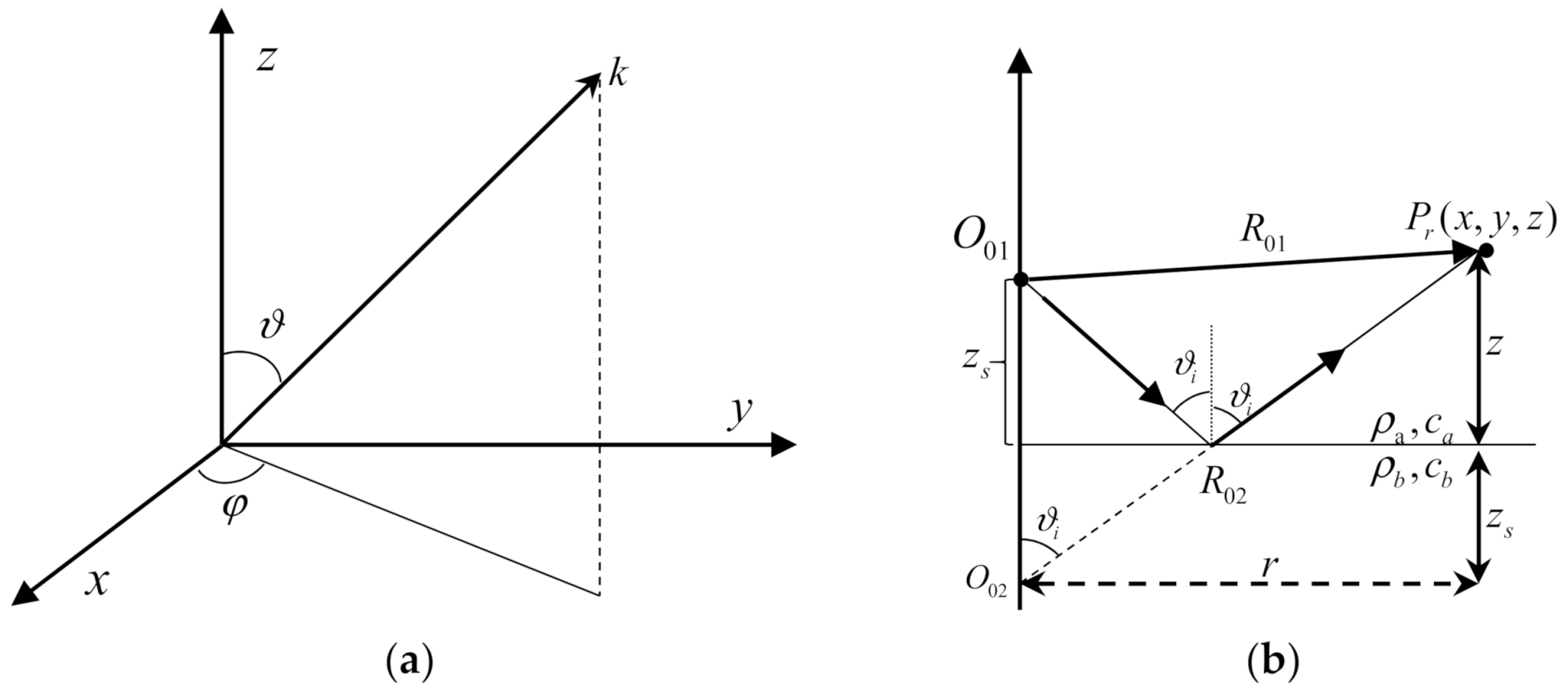
As shown in Figure 2a, we perform the wavenumber domain conversion in this 3D space and the components $k_x$ and $k_y$ of the wave vector k can be replaced by integration over the angles $\vartheta$ and φ as follows:

$$k_x=k\sin \vartheta \cos \phi ,k_y=k\sin \vartheta \sin \phi ,k_z=k\cos \vartheta =\sqrt{k^2-k_x^2-k_y^2},$$

(10)

The angle range of φ is (0, 2π). According to Equation (10), when$k_x=k_y=0$, $k_z=k$ is obtained. Additionally, ${\mathrm{k}}_{\mathrm{z}}=\mathrm{i}\infty$ when ${\mathrm{k}}_{\mathrm{y}}\to \pm \infty$, so that the angle range of $\vartheta$ can be expressed as (0, π/2−i∞). With the use of the variable transformation formula $\frac{d{k}_{x}d{k}_y}{k_z}=ksin\vartheta d\vartheta d\phi$, Equation (9) can also be written in the following form:

$$\frac{e^{ikR}}{R}=\frac{ik}{2\pi }{\displaystyle {\int }_0^{(\pi /2)-i\infty }{\displaystyle {\int }_0^{2\pi }{e}^{i(k_{x}x+k_{y}y+k_{z}z)}}}\sin \vartheta d\vartheta d\phi ,$$

(11)

Up to this point, we know that different orders of plane waves are decomposed from the spherical wave and reflecting at the fluid–fluid interface with different incident angles. Each order of plane wave on the interface satisfies the Snell law for reflection and should be multiplied by the corresponding reflection coefficient $\mathrm{V}(\vartheta )$.

Assuming m = 0, as shown in Figure 2b, for the first time the spherical wave of the sound source interacts with the interface, the physical source $O_{01}$ is mirrored by the interface to the first image source $O_{02}$. In this case, the path of the sound field of the source $O_{02}$ is $R_{02}=\sqrt{r^2+z_{02}^2}$.

Based on Equations (10) and (11), the sound field of the spherical wave radiated by the image source $O_{02}$ on the fluid–fluid interface can be found from the following equation

$${\mathrm{V}}_2\left(\vartheta \right)\frac{e^{ik{R}_{02}}}{R_{02}}=\frac{ik}{2\pi }{\displaystyle {\int }_0^{(\pi /2)-i\infty }{\displaystyle {\int }_0^{2\pi }{e}^{ik(x\sin \vartheta \cos \phi +y\sin \vartheta \sin \phi +z_{02}\cos \vartheta )}}}{\mathrm{V}}_2\left(\vartheta \right)\sin \vartheta d\vartheta d\phi ,$$

(12)

On the xoy plane, let $x=rcos{\phi }_1$, $y=rsin{\phi }_1$, which results in the following:

$$\begin{array}{l}{\displaystyle {\int }_0^{2\pi }{e}^{ik\sin \phi (x\cos \phi +y\sin \vartheta )}d\phi }={\displaystyle {\int }_0^{2\pi }{e}^{ikr\sin \phi (\cos {\phi }_1\cos \phi +\sin {\phi }_1\sin \phi )}}d\phi \\ \begin{array}{cccc}\begin{array}{ccc}& & \end{array}& & & \end{array}={\displaystyle {\int }_0^{2\pi }{e}^{ikr\sin \phi \cos (\phi -{\phi }_1)}}d\phi ,\end{array}$$

(13)

According to the definition of the nth order Bessel function

$$J_n(x)=\frac{1}{2\pi i^n}{\displaystyle {\int }_0^{2\pi }{e}^{ix\cos \theta }}\cos (n\theta )d\theta ,$$

(14)

Here, we take n = 0, and the above equation can be rewritten as follows:

$${\displaystyle {\int }_0^{2\pi }{e}^{ik\sin \phi (x\cos \phi +y\sin \vartheta )}d\phi }=2\pi J_0(kr\sin \phi ),$$

(15)

According to Equation (15), Equation (12) can be expressed as follows:

$${\mathrm{V}}_2\left(\vartheta \right)\frac{e^{ik{R}_{02}}}{R_{02}}=ik{\displaystyle {\int }_0^{(\pi /2)-i\infty }{e}^{ik{z}_{02}\cos \vartheta }{J}_0}\left(kr\sin \vartheta {)\mathrm{V}}_2\right(\vartheta )\sin \vartheta d\vartheta ,$$

(16)

Similarly, we can obtain the reflected sound field of other image sources. The expression is also conveniently transformed by changing the limits of integration and replacing the Bessel function by Hankel functions. For this, we note that

$$\begin{array}{l}{J}_0(x)=(1/2)\left[H_0^{(1)}(x)+H_0^{(2)}(x)\right]\\ \begin{array}{cc}& \end{array}=(1/2)\left[H_0^{(1)}(x)-H_0^{(1)}(-x)\right],\end{array}$$

(17)

We apply the relation to each image source. The spherical waves are decomposed into plane waves with various orders by using the double Fourier integration as follows:

$$\frac{e^{jk{R}_{mn}}}{R_{mn}}{V}_2(\vartheta )=\frac{ik}{2}{\displaystyle {\int }_{-(\pi /2)+i\infty }^{(\pi /2)-i\infty }{H}_0^{(1)}(kr\sin \vartheta )}{e}^{ik{z}_{mn}\cos \vartheta }{V}_2(\vartheta )\sin \vartheta d\vartheta$$

(18)

The reflected sound field of the spherical wave is decomposed into the plane wave by Equation (18). We consider the reflection at an interface separating two homogeneous fluid media with the reflection coefficients, which can be written in the form:

$$V_2(\vartheta )=\left\{\begin{array}{l}\frac{\mathcal{l}\cos \vartheta -\sqrt{{\beta }^2-{\sin }^2\vartheta }}{\mathcal{l}\cos \vartheta +\sqrt{{\beta }^2-{\sin }^2\vartheta }},\left|\sin \vartheta \right|\le \beta \\ 1\begin{array}{cc}& ,\left|\sin \vartheta \right|>\beta \end{array}\end{array}\right.,$$

(19)

where $\mathcal{l}={\rho }_b/{\rho }_a$, $\beta =c_a/c_b$, $\vartheta$ represent the incident angle of the plane wave.

The seabed surface of shallow water is covered with a layer of non-condensable solid material, which is deposited by several rivers, so it is reasonable to simulate the seabed sediment as a liquid. Further, the attenuation also becomes a significant loss factor for waterborne energy. Hence, in this case, it is crucial for realistic modeling of the propagation characteristics that bottom attenuation is taken into account to improve the accuracy of the sound propagation model. Here, we describe the sound attenuation effect with the complex sound speed as follow:

$$\widetilde{c_b}=\frac{c_b}{1+\mathrm{j}\frac{{\alpha }_b}{2}}$$

(20)

where ${\alpha }_b$ is the absorption coefficient in the fluid seabed. The absorption coefficient of sound in the seabed is measured in a wavelength, which is given by the expression ${\alpha }_{\lambda }\left(\mathrm{dB}/\mathsf{\lambda }\right)=27.3{\alpha }_b$ [25].

By substituting Equation (18) into Equation (1), we can obtain the GF in an explicit form

$$\begin{array}{l}G(r,z)=\frac{ik}{2}{\displaystyle {\int }_{-(\pi /2)+i\infty }^{(\pi /2)-i\infty }{H}_0^{(1)}(kr\sin \vartheta )}\cdot \left[e^{ik\cos \vartheta (z-z_s)}+V_2({\vartheta }_i)e^{ik\cos \vartheta (z+z_s)}\right.+V_1{e}^{ik\cos \vartheta (2H-z-z_s)}\\ \begin{array}{ccc}& & \end{array}\left.+V_1{V}_2({\vartheta }_i)e^{ik\cos \vartheta (2H-z+z_s)}\right]{\displaystyle \sum _{m=0}^{\infty }{\left(V_1{V}_2({\vartheta }_i)\right)}^m}{e}^{2m\cdot ik\cos \vartheta \cdot H}\sin \vartheta d\vartheta ,\end{array}$$

(21)

By combining with the Simpson algorithm for complex integrals [26], the GF can be solved efficiently. Additionally, the sound field of the radiator generally focuses on the sound pressure level (SPL), which is defined as follows:

$$SPL=20\times \log 10\frac{p}{p_{ref}}(\mathrm{dB})$$

(22)

where $= 1\times {10}^{-6}$ Pa is the reference sound pressure in water.

3. Theoretical Model Verification

A typical sound propagation model in the Pekeris waveguide is established to verify the Green functions described by the ISM, as shown in Figure 3, which consists of a point source that is 30 m in depth, where the upper surface is the pressure released, the depth of homogeneous water is 100 m, and the density and the sound speed are ${\rho }_a$= 1024 kg/m³ and $c_a$ = 1500 m/s, respectively. The seabed in the Pekeris waveguide is regarded as an infinite half-space liquid with the density and the sound speed of ${\rho }_b$ = 2000 kg/m3 and $c_b$= 1800 m/s, respectively, and the sound absorption in the seabed is also considered. The depth of each receiver is $z_i$ and the horizontal interval is 1 m.

From the configuration of the Pekeris waveguide shown in Figure 3, it is clear that the upper boundary is the Dirichlet boundary (i.e., the reflection coefficient is ${\mathrm{V}}_1=-1$). The seabed is an infinite liquid half space, and the interaction between the sound field and the fluid–fluid interface can be described by using the reflection coefficient. As shown in Figure 4, Equation (19) is utilized to calculate the reflection coefficient of the plane wave at the interface versus the incident angle for different absorption coefficients of the seabed.

It can be observed that the reflection coefficient is positively related to the incident angle $\vartheta$. When the liquid seabed does not contain sound absorption, there is an incident angle (i.e., the critical angle) so that the sound field on the interface appears to be a total reflection, the reflection coefficient is constant at 1, and the critical angle is $\vartheta =\mathrm{arc}\sin \left({\mathrm{c}}_{\mathrm{a}}/{\mathrm{c}}_{\mathrm{b}}\right)\approx {56}^{\circ }$. In contrast, when the medium contains acoustic absorption with ${\alpha }_{\lambda }=0.5\mathrm{dB}$/$\mathsf{\lambda }$, ${\alpha }_{\lambda }=1.0\mathrm{dB}$/$\mathsf{\lambda }$, and ${\alpha }_{\lambda }=2.0\mathrm{dB}$/$\mathsf{\lambda }$, the reflection coefficient is a value that varies with the angle of incidence, and total reflection no longer occurs. The reflection coefficients are approximately the same for angles less than the critical angle (i.e., 56°). For angles above the critical angle, the reflection coefficients corresponding to different absorptions vary considerably. Therefore, the spherical waves carry plane waves in different directions and incident angles on the fluid–fluid interface with the sound absorption. The reflection coefficients of the plane waves are different in each direction. Although in the range of 0–10° the reflection coefficient can all be approximated as 0.41 (i.e., it is reasonable that the reflected sound field at the receiver in the range of $\left.r\le 0.18(z_s+z\right)$ can be calculated using Equation (1)), the distance of the receiver is too close to be used to accurately describe the reflected sound field in the Pekeris waveguide. Therefore, to make the ISM more accurate for sound field calculations over the whole distance, it is necessary to decompose the spherical wave into plane waves with different incident angles. The reflected sound field of the spherical wave from the point source is solved according to Equation (18), and finally, the reflected sound field of a physical source and image sources are summed by Equation (1). Thus, the sound field of a point source (i.e., the GF) in the Pekeris waveguide at any field point is obtained by this rigorous ISM.

The cutoff effect will occur in the sound propagation due to the limitation of the upper and lower boundaries of the shallow water (i.e., the sound field below the cutoff frequency cannot propagate in long distances), and the sound propagation frequencies of the order normal modes in the Pekeris waveguide can be above the cutoff frequency $f_n$ given by [22]

$$f_n=\frac{\left(2n-1\right)c_a{c}_b}{4H\sqrt{c_b^2-c_a^2}},$$

(23)

The propagation frequencies corresponding to the first 6-order normal modes are presented in

Table 1. The propagation frequencies of first 6-order normal modes.

n	1	2	3	4	5	6
$f_n$/Hz	6.78	20.35	33.92	47.49	61.06	74.62

. When the propagation frequency is lower than the first-order propagation frequency (e.g.,$f_1=6.78\mathrm{Hz}$) the sound field will decay rapidly with the propagation distance and cannot travel far away. To fully compare the calculation accuracy of the ISM for the sound field in the near and far fields, the selected frequencies are 25 Hz, 50 Hz, 100 Hz, and 200 Hz, and the ${\alpha }_{\lambda }=0.5\mathrm{dB}/\mathsf{\lambda }$.

As shown in Figure 5, the SPLs of the point source in this waveguide are calculated by adopting the rigorous ISM, and these results are compared with the theoretical solutions calculated accurately by the mature Scooter calculation program based on WI techniques; the depth of each receiver is half of the water depth (i.e., $z_i=50\mathrm{m}$). It can be seen that the results between the ISM and theoretical solutions are in good agreement in the near and far fields. The ISM considers the upper and lower boundaries through the image sources generated by mirror reflection, and the total sound field is expressed by the physical source and the various image sources. Further, on the fluid–fluid interaction surface, the spherical wave is decomposed into plane waves with various orders through Equation (18), and then the identified reflection coefficient of the plane wave is used to describe the reflection effect on the sound field. Thus, the ISM is an exact solution and simpler than WI, which can handle the near-to-far field problem well.

As shown in Figure 6, where the SPL in the xor plane is provided as a comparison value for the results calculated by the presented method and WI, the frequencies are chosen to be 25 Hz and 100 Hz. The modal interference patterns of the sound field calculated by the two methods are identical over the entire calculated distance. For example, when the frequency is 25 Hz, which is more than the cutoff frequency, there are two modes, as shown in Table 1. Thus, two normal modes appear in the depth direction of the radiated sound field in Figure 6a,b. Additionally, there are more orders of modal interference patterns when the frequency increases to 200 Hz, as shown in Figure 6c,d.

Sound propagation in the Pekeris waveguide is generally concerned with the far field, where the sound field will interact with the seabed tens to thousands of times, and the sound losses of multiple sound paths will sum to significant levels, so the effect of seabed absorption on sound field propagation must be taken into account. As shown in Figure 7, the SPL is calculated using this method for different cases with three absorption coefficients, where all receivers are 50 m and the selected frequency is 20 Hz. It can be seen that at a short distance, for example, in the 0–700 m range, the variation in SPL for different absorption coefficients is minor. Because there are a small number of interactions between the sound field and the lossy seabed, there is not a significant effect on the whole sound propagation, which is dominated by geometrical spreading loss. However, the sound propagation loss from multiple contacts with the seabed accumulates to a considerable level as the propagation distance increases, resulting in differences in the SPL curves with different coefficients becoming gradually visible. Thus, it is concluded that the sound loss increases more rapidly with increased ranges for the lossy seabed, and the modal interference length is slightly different for the different seabed absorption coefficients.

4. Conclusions and Future Work

The sound field of a point source (i.e., GF) directly satisfies the boundary conditions on the free surface and the horizontal parts of the seabed boundary and establishes the sound transfer relationship between the vibration source and the receiver, which can be utilized to provide a concise mathematical expression and eases the efficient computation for acoustic radiation problems in shallow water with the aid of the Helmholtz integral equation.

In this paper, an efficient GF for acoustic problems in shallow water was developed by the rigorous ISM model, in which the interaction between the spherical wave sound field and the liquid seabed of the Pekeris waveguide was established based on the classical ray theory and wave acoustics, and the sound loss due to multiple interactions with a lossy seabed was also taken into account. Taking the source field of a point source in the Pekeris waveguide as an example, the SPL and the sound modal interference calculated by this method were compared with those presented by the standard WI. After verifying the accuracy of the GF for calculating the sound field over the whole distance, the influence of lossy seabed on the sound field of a point source was investigated, and it was found that sound loss increased more rapidly with an increase in range for the lossy seabed, due to the sound absorption of the seabed, and the modal interference length was slightly different for the lossy seabed.

This paper proposes a GF that is more adaptable to near- and far-field acoustic problems. In the future, on one hand, for a simple point source, investigations on sound propagation, long-range localization, and geoacoustic inversion in shallow water can be conducted efficiently. On the other hand, for large elastic radiators, computational methods such as the Helmholtz integral equation, the boundary element method, the equivalent source method, and the hydroelasticity theory can be combined to further promote the development of acoustic cloaking design, near-field acoustic field measurement, and target identification for underwater vehicles.