Tool Health Monitoring Using Airborne Acoustic Emission and Convolutional Neural Networks: A Deep Learning Approach

Abstract

Tool health monitoring (THM) is in great focus nowadays from the perspective of predictive maintenance. It prevents the increased downtime due to breakdown maintenance, resulting in reduced production cost. The paper provides a novel approach to monitoring the tool health of a computer numeric control (CNC) machine for a turning process using airborne acoustic emission (AE) and convolutional neural networks (CNN). Three different work-pieces of aluminum, mild steel, and Teflon are used in experimentation to classify the health of carbide and high-speed steel (HSS) tools into three categories of new, average (used), and worn-out tool. Acoustic signals from the machining process are used to produce time–frequency spectrograms and then fed to a tri-layered CNN architecture that has been carefully crafted for high accuracies and faster trainings. Different sizes and numbers of convolutional filters, in different combinations, are used for multiple trainings to compare the classification accuracy. A CNN architecture with four filters, each of size 5 × 5, gives best results for all cases with a classification average accuracy of 99.2%. The proposed approach provides promising results for tool health monitoring of a turning process using airborne acoustic emission.

1. Introduction

According to the World Bank statistics, the manufacturing industry of the world had 13.945 trillion U.S dollars’ worth in 2018 with a 2.708% annual growth potential [1,2]. Cutting-edge manufacturing industries like computer numeric control (CNC) machines play a major role toward faster and more efficient manufacturing processes. Component degradation of a machine has a significant effect on the performance of the machine, whereas its tool is the direct affecter of the performance of the machining quality, yield, and time factors. Bad tool health makes the machine or workpiece chatter and overheat, which are highly undesirable induced malfunctioning phenomena for the machining processes. Tool wear has numerous types that result in poor machining finishes and adverse machining outcomes. Abrasive wear in tools occurs due to periodic degradation, resulting in blunt tool edges. Thermal cracking is another problem that occurs in CNC tools as a result of temperature flux, and is very harmful to the undergoing process. Tool fracture is the type of tool wear that is caused by sudden breakage of the tool. There are multiple reasons for tool fractures such as inappropriate machining speed, feed, or improper work-piece or tool handling. Moreover, due to excessive vibrations or shock-loadings in the machining process, chipping occurs, which adversely affects the workpiece finish. These tool degradations should be monitored actively to avoid adverse consequences. In common practice, the tool health monitoring is done in the machine offline state, eventually increasing the machine downtime along with the increased risk of unpredicted sudden tool damages that could result in serious human injuries, work-piece, or machine damage. The CNC machining operation could significantly be increased using the robust online tool health monitoring system that would ensure real-time tool condition monitoring yielding toward minimal machine downtime or breakdown time. Whereas the utilization of CNC tools can be assessed through the worldwide CNC tool production industry profit figures for the year of 2016 to be around 67.6 billion Euros, the compound annual growth rate (CAGR) of this industry is predicted to be 9% [3].

Ray et al. [4] proposed the hybrid technique that uses acoustic emission and the hidden Markov model (HMM) for tool wear prediction in titanium alloy (Ti-5553) during the milling process. Acoustic emission (AE) data of the milling process was acquired using an AE sensor that was installed at the back of the workpiece fixture. Machining parameters involving the axial depth of cut, radial depth of cut, spindle speed, and feed rate were set at 0.03 mm, 0.7 mm, 5082 rpm, and 4.268 m/min, respectively. After machining for a pre-determined time, tools were measured using an Alicona 3D optical microscope to classify various levels of wear, and once the state of the tools was confirmed, these tools were used to cut a material specimen while collecting monitoring signals from the process. Time-domain features like root mean square (RMS), mean, skewness, kurtosis, and peak signal values were extracted from AE recordings of the milling process and were presented to principal component analysis (PCA) for dimensionality reduction of the features. Four training states, new, used, worn-out, and damaged, were obtained by using multi-class support vector machines (SVM) on recorded data. The hidden Markov model was trained using a transition matrix and showed an accuracy of 98% for tool wear prediction. Cunji et al. [5] proposed a wireless sensor-based technique for tool condition monitoring in dry milling operations. The proposed technique uses a triaxial accelerometer to capture vibration signals that were further de-noised by wavelet analysis, followed by the extraction of time domain, frequency domain, and time–frequency domain features. Optimal feature selection was made based on Pearson’s correlation coefficient (PCC), and these optimal features were used to train the Back-Propagation Neural Network (BPNN), Radial Basis Function Neural Network (RFNN), and Neuro Fuzzy Network (NFN) to predict tool wear. The NFN showed the best performance for the prediction of tool wear with a mean squared error (MSE) of 3.25 × 10⁻⁴ and mean absolute percentage error (MAPE) of 0.0224. The experimental setup involved a mini-CNC milling machine, tempered steel (HRC52) workpiece, micro-grain carbide two-flute end milling cutter coated with multilayer coatings of titanium aluminum nitride (TiAlN), a wireless triaxial accelerometer mounted on the workpiece to measure the vibration, and a wireless base station to process the vibration signal and transmit these signals to a computer through the local area network (LAN).

Xiaozhi et al. [6] proposed the use of acoustic emission for tool condition monitoring in the turning process. The proposed technique makes use of acoustic emission and wavelet analysis to monitor tool wear during turning operations. Machining tests were carried out using an NC turning center, mild steel workpiece, and tungsten carbide finishing tool. Experiments were performed using sharp and worn-out tools with different machining conditions. A piezoelectric AE sensor was mounted on the tool holder with a light coating of petroleum jelly to ensure good acoustic emission coupling. A high-pass filter was applied to the acquired AE signals to wipe out the low-frequency noise components. Time-domain and frequency-domain plots for the acquired AE signals of the sharp tool were distinguishable from the plots of the worn-out tool. The sixth-scale wavelet resolution coefficient norm was extracted for the sharp and worn-out tool separately using wavelet analysis. The coefficient norm of the signals from the sharp tool was much more stable than that of the worn-out tool. Dimla et al. [7] proposed a sensor fusion and artificial neural network (ANN)-based approach for tool condition monitoring (TCM) in metal cutting operations. The proposed technique uses the Kistler triaxial accelerometer and Kistler charge amplifier to record the static cutting force, dynamic cutting force, and vibration signals during turning operation on new and worn-out tools. The obtained data were used to investigate the classification capability of simple Multi-Layer Perceptron (MLP) neural network architectures to the detection of tool wear. Obtained results showed that a classification accuracy of well over 90% was attainable.

A major advantage of using acoustic emission (AE) as a tool condition monitoring technique is that the frequency of AE signals is much more dominant than those of machine vibrations and environmental noise. Back-Propagation Neural Networks (BPNNs) have been extensively used to model relations between tool states and signal features extracted from the acoustic emission sensor, vibration sensor, and dynamometer [8,9,10]. However, industrial tool condition monitoring cannot be performed via BPNN, due to its slow computing speed in online modelling applications. Due to their improved on-line computing speed, Hongli et al. [8] proposed the use of a Localized Fuzzy Neural Network (LFNN) for tool condition monitoring in turning operations. Experiments were conducted on a conventional lathe to acquire force signals with a dynamometer and AE signals with an AE transducer. Time domain, frequency domain, and frequency–time domain features were extracted from both force and AE signals. Twelve relevant features were selected using the synthesis coefficient approach as a feature selection technique. Adaptive learning was used to train an LFNN to model the relationship between extracted features and tool wear amount with high precision and good on-line computing speed.

Several time-domain and frequency-domain features of acoustic emission released during machining have been used with conventional neural networks for tool health monitoring applications. The proposed approach uses time and frequency domain-fused spectrographs with deep learning-based convolutional neural networks for tool health monitoring applications. This research presents a novel and low-cost technique for the tool health monitoring with an efficient data acquisition process. The proposed method uses a typical microphone as an airborne acoustic emission sensor to acquire the CNC turning operation signals and employs deep learning techniques to predict tool condition. Multiple types of materials and tools are used for machining purposes in order to predict the tool health and validate the deep learning algorithm. It is for the first time that convolutional neural networks (CNN) are being used along with the visual spectrum of an acoustic signal to categorize tool health. Different types of performance evaluations with accuracy comparisons on a fairly high variety of materials and tools are discussed. The methodology and proposed technique are being discussed in detail in the next section.

2. Proposed Technique

Figure 1 illustrates the comprehensive flow chart of the proposed technique. At first, the machining process AE signal is acquired using a standard microphone. Then, the raw AE signals are preprocessed to convert it into two-dimensional images. Later, CNN architecture is designed with different layers. After setting up the parameters and hyper-parameters according to the proposed design requirement, the images are fed to the architecture, to begin with the training. Finally, the classification results are validated after each training and the performance of the algorithm is evaluated.

3. Background Theory

3.1. Convolutional Neural Network (CNN)

A convolutional neural network (CNN) is a type of neural network that is more specialized for the training of visual or image type data sets. Like an ordinary neural network, the CNN has an input layer, numerous hidden layers, and an output layer. The major differences of CNNs from the rest of the neural networks reside in the technique to have optimized the minimal number of weights to reduce the training time, while these weights are connected in the local spatial domain, and secondly, it smartly selects the features for training on its own from the input images [11], which are the abstract representation of input data at various stages and structuration. Figure 2 shows the difference between a typical neural network and a CNN neural network framework.

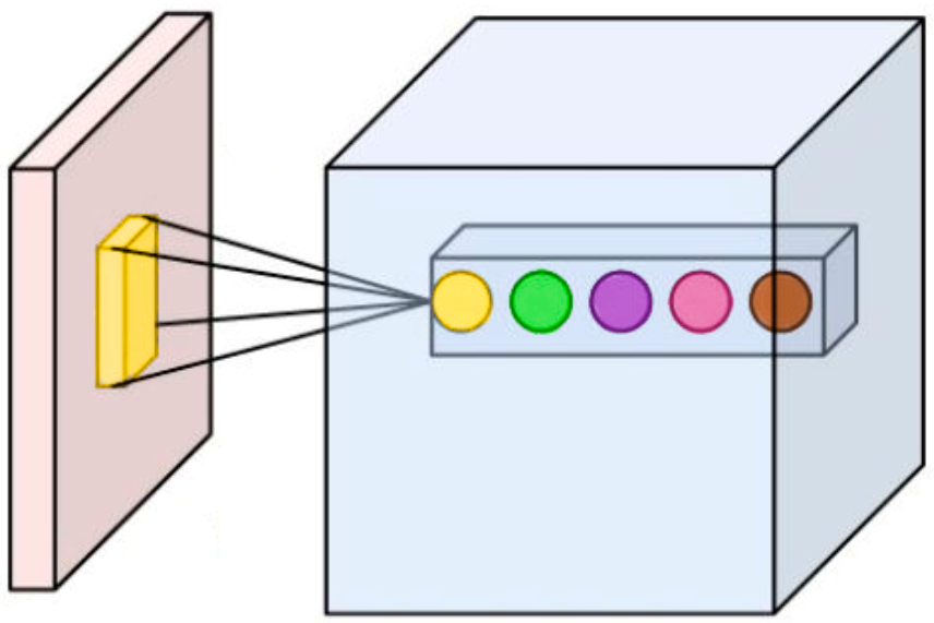
There are several layers of CNN among which some are commonly used layers. The convolutional layer is the main and foremost layer of the CNN architecture. The integral part of this layer is the small patches known as filters or kernels. These filters have a certain length and height, but the depth for a color image is threefold due to three channels; red, green, and blue. The parameters such as the number and size of filters rely on the forward-fed layer parameters such as width, height, and depth of the structure taken as input to the particular layer and intuitive selection [13]. Smaller filter size helps in retaining the critical information [14,15]. On the input layer or the previous layer of the convolutional layer, each filter convolves through the width and height of the previous input structure, and then computes a dot product between filter numeric entries and current common regional values on the input, resulting in the formation of an activation map in two-dimensional spatial domains. The activation maps generated are equal to the number of filters used. Figure 3 shows the activation maps that are stacked in depth to produce the resulting output of the layer. The activation unit can be represented by the equation below.

$$x_u^{k+1}={\displaystyle \sum }_i{w}_{k,u}^{k+1}{x}_u^k+b_k$$

(1)

where $x_u^k$ are the activations, $w_{k,u}^{k+1}$ is the weight of the entity of activations, b is the bias of the layer, k is the layer, and u is the individual entity.

The resulting output of the single convolutional layer depends upon hyper-parameters such as stride, zero padding, and depth. Stride represents the number of pixels the filter jumps after every convolution step on the input. The smaller the stride, the greater the dimension of the output. Zero padding is used to pad the boundary of the input with zeros in order to preserve the output area the same as the input area, whereas depth is controlled by the number of filters being convolved with the input volume. For the square-shaped input layer and filter, the area of the output could be found using the following equation:

$$L_o=\frac{L_i-F+2Z}{S}+1$$

(2)

where $L_i$ and $L_o$ are the input and output lengths for the square $L_i^2$ and $L_o^2$ areas, respectively, $F$ is the filter length for the $F^2$ area, $Z$ is the zero padding, and $S$ is the stride. The number of neurons of the corresponding layer connected to the input layer could be found using the following equation:

$$N_n=L_o^2\times N_F$$

(3)

where $N_n$ and $N_F$ are the number of neurons and filters, respectively. The number of weights for each neuron in the convolutional layer can be found using the following equation:

$$N_w=L_F^2\times D_i$$

(4)

where $N_w$ is the number of weights, $L_F^2$ is the filter area, and $D_i$ is the depth of the input layer. The ReLU Layer brings nonlinearity to the linear structure after convolutional layer computations. The ReLU activation function proved to be more efficient than the traditional activation functions [16], to be less prone to decrease the accuracy, and to improve the gradient fall due to which the lower layers of the system perform slow computations. The ReLU function zeroes the negative activations in the input layer with the following function:

$$f\left(x\right) =\max \left(0,x\right)$$

(5)

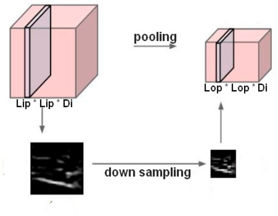
The pooling layer is used after the ReLU layer to down-sample the fed input layer, thus having the role of controlling the overfitting and reducing the parameters in the CNN architecture. The downsampled output of the pooling layer could be found using the following equation:

$$L_{op}= \left(L_{ip}-L_{PF}\right)/S+1$$

(6)

where $L_{op}$ and $L_{ip}$ are the length of the square-shaped output and input area, respectively, and $L_{PF}$ is the pooling filter length. $L_{PF}$ is chosen to be minimal to avoid too much deterioration of input layer details. The depth, being the third constituent of input and output with the area, remains constant in the volumetric details of the layer. Figure 4 shows the pooling layer structure of the CNN.

The fully connected layer is the final layer of the CNN architecture that performs the task of forming the vector of probabilities for the input image, showing how likely the input falls among all classes. It is called fully connected due to the neurons of this layer being fully connected to the activations of the fed input layer. Generally, the fully connected layer is followed by the softmax function that is the unit activation function for the output. It is considered as the generalization of the logistic sigmoidal function for the multiple classes [17,18].

$$P\left(C_r|x,\theta \right) =\frac{P\left(x,\theta |C_r\right)P\left(C_r\right)}{{{\displaystyle \sum }}_{j=1}^{g}P\left(x,\theta |C_j\right)P\left(C_j\right)}=\frac{\exp \left(a_r\left(x,\theta \right)\right)}{{{\displaystyle \sum }}_{j=1}^g\exp \left(a_j\left(x,\theta \right)\right)}$$

(7)

where ${\displaystyle \sum }_{j=1}^{g}P\left(C_j|x,\theta \right) =1$, $0\le P\left(C_r|x,\theta \right)\le 1$ and $a_r=\ln \left(P\left(x,\theta |C_r\right)P\left(C_r\right)\right),P\left(x,\theta |C_r\right)$ are the conditional probabilities of the known sample class r, and $P\left(C_r\right)$ is the prior probability of the class.

3.2. Spectrogram

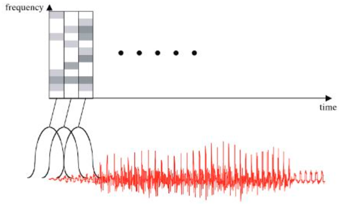
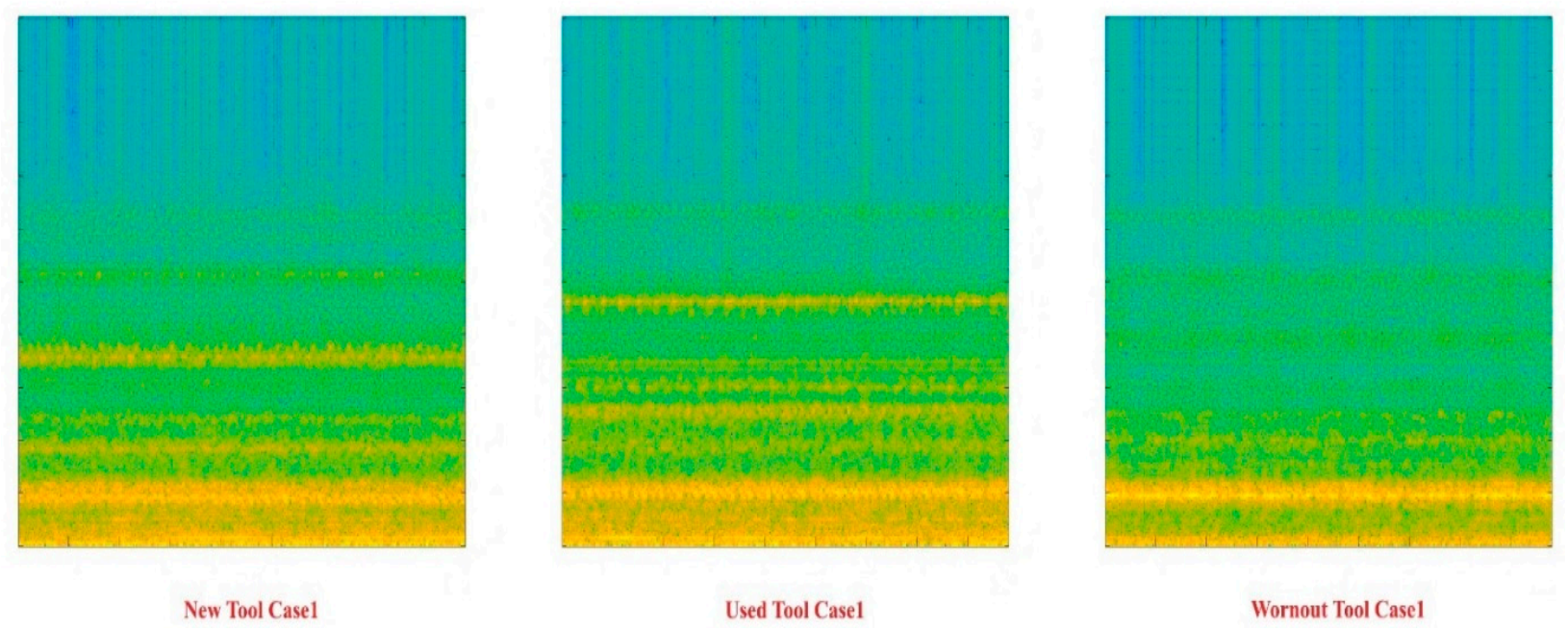
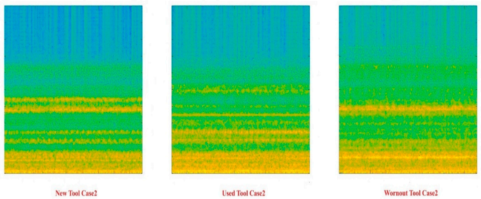
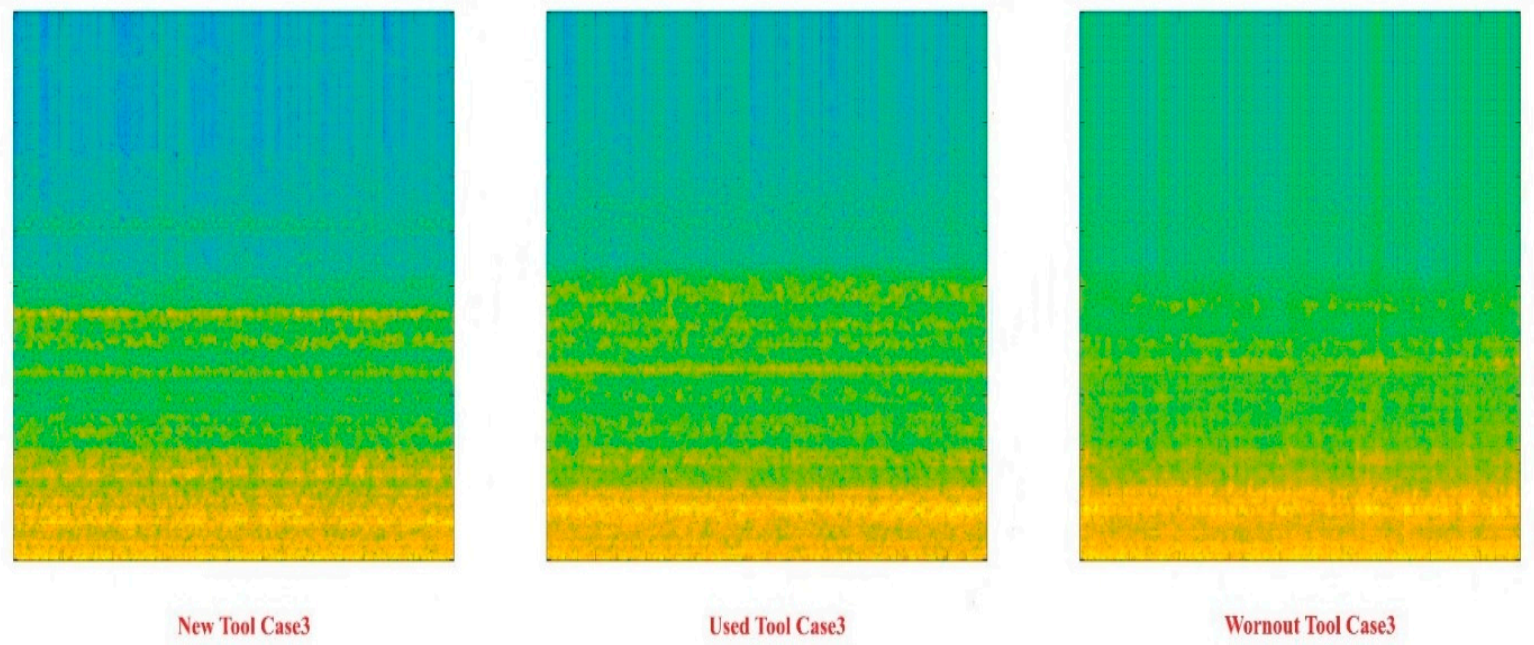
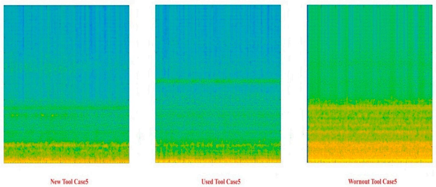
A spectrogram is originated by the sequential computations of short-time Fourier transforms (STFT) together with the time domain signal. The shades of colors in the spectrogram are the logarithmic energy representation of discrete Fourier transforms (DFT) windowed on a particular time and frequency of the signal [19]. In the representation of the spectrogram, the time is plotted on the horizontal axis and the frequency on the vertical axis, and the energy intensity is displayed using color representation. Higher energy levels are shown with yellow color saturation and lower energy levels are shown with blue color saturation. The greater the energy bands lying on the base of the frequency axis, the greater the energies at the lower frequencies. Figure 5 illustrates the construction of a spectrogram from a time-domain signal where small windows of the signal are being converted into color bands of the spectrogram. It becomes difficult to mathematically model the acquired AE signals; therefore, derived signal parameters become a good option. Spectrograms have recently been used by Ahmed et al. [20] to identify six different human activities using the measured Channel State Information (CSI).

4. Experimentation

4.1. Experimental Setup and Data Acquisition

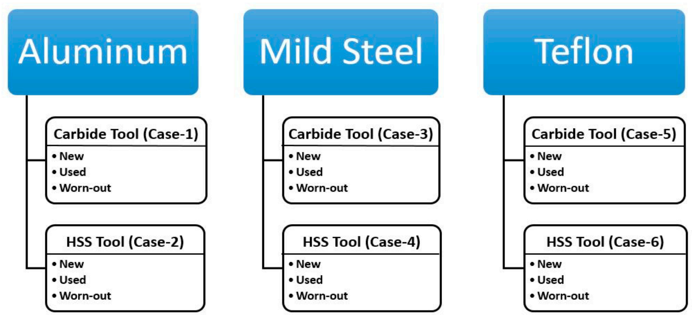
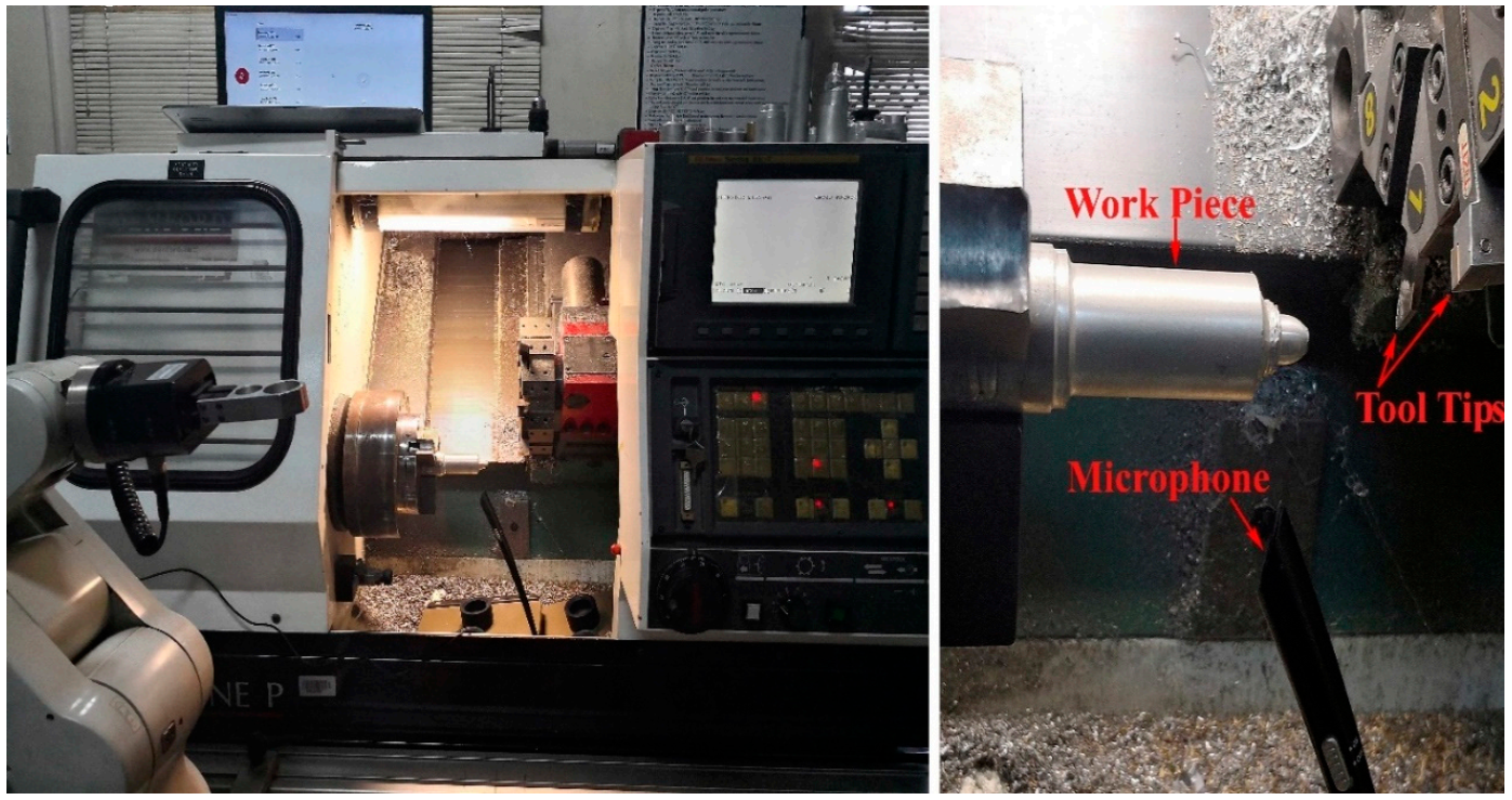
Experiments were performed in the Industrial Automation Lab of College of EME, National University of Sciences and Technology, Islamabad, Pakistan. A Denford Cyclone P with a built-in Fanuc 21i-TA control, Computer Numerical Control (CNC) lathe machine was used to perform the turning operation on three types of materials: Aluminum, mild steel and Teflon, with two types of tooltips: Carbide and high-speed steel (HSS). Figure 6 shows the complete experiment categorization. In total, six cases were formed with all the combinations of tools and workpieces used during experimentation. For classification purposes, the acoustic emission signals of the new, used, and worn-out tool were recorded using a standard microphone with a sampling frequency of 44,100 Hz. The turning operation parameters are shown in

Table 1. Turning operation parameters.

Feed Rate	RPM	Depth of Cut
200 mm/min	1500 rev/min	1 mm

.

Figure 7 shows the complete machining and data acquisition process where a workpiece is gripped by a chuck of the CNC machine for turning operation, and the tool holder with different tool types for the selection of tool material and shape can be observed. The typical microphone used as an airborne acoustic emission sensor is placed between the workpiece and tool with a minimal distance between machining location and microphone, in order to acquire the AE signal with the least background noise. The signal is being recorded with a built-in Windows^® 10 voice recording application through a laptop having a 3.5 mm audio jack.

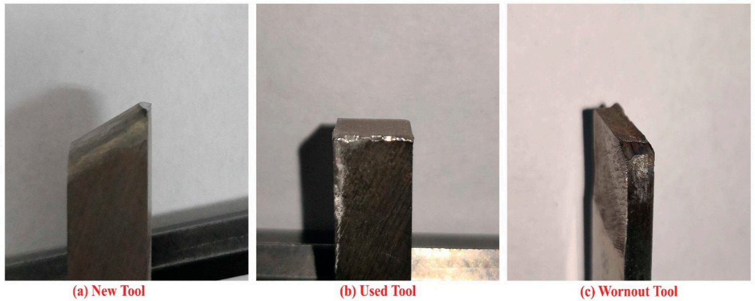
Figure 8 shows all three types of workpieces on which the turning operation has been performed with two different types of tools. Figure 9 and Figure 10 show all the categories of the carbide and HSS tool utilized as new, used, and worn-out tool conditions. In the literature, flank and carter wear of the tools are mostly discussed, as they occur most during the machining processes and are major factors leading to workpiece surface roughness. The cutting force of a tool affects the tool wear, while interestingly, cutting force itself is dependent on tool condition. The greater the flank wear, the greater the tool and workpiece inter-friction would be, eventually increasing the thermal signature of both surfaces, resulting in higher cutting forces [21]. Cutting force also greatly relies on machining parameters. Higher feed rates and deeper depths of cuts generate a greater cutting force [22], tool wear and workpiece surface roughness [23]. A carbide tool is harder while a HSS tool is tougher; a carbide tool has more abrasion resistance while the HSS tool has more local deformation resistance [24]. On the other hand, workpiece material also greatly affects the tool life [25]. In this experiment, the hardest workpiece material used is mild steel, aluminum being moderate and Teflon being the softest. The worn-out tool category has had artificially induced mechanical fractures through a hammer, while used tool category tools have been in use at the Lab of College before the experimentation performed with considerable usage cycles.

4.2. Acoustic Emission Signals Preprocessing

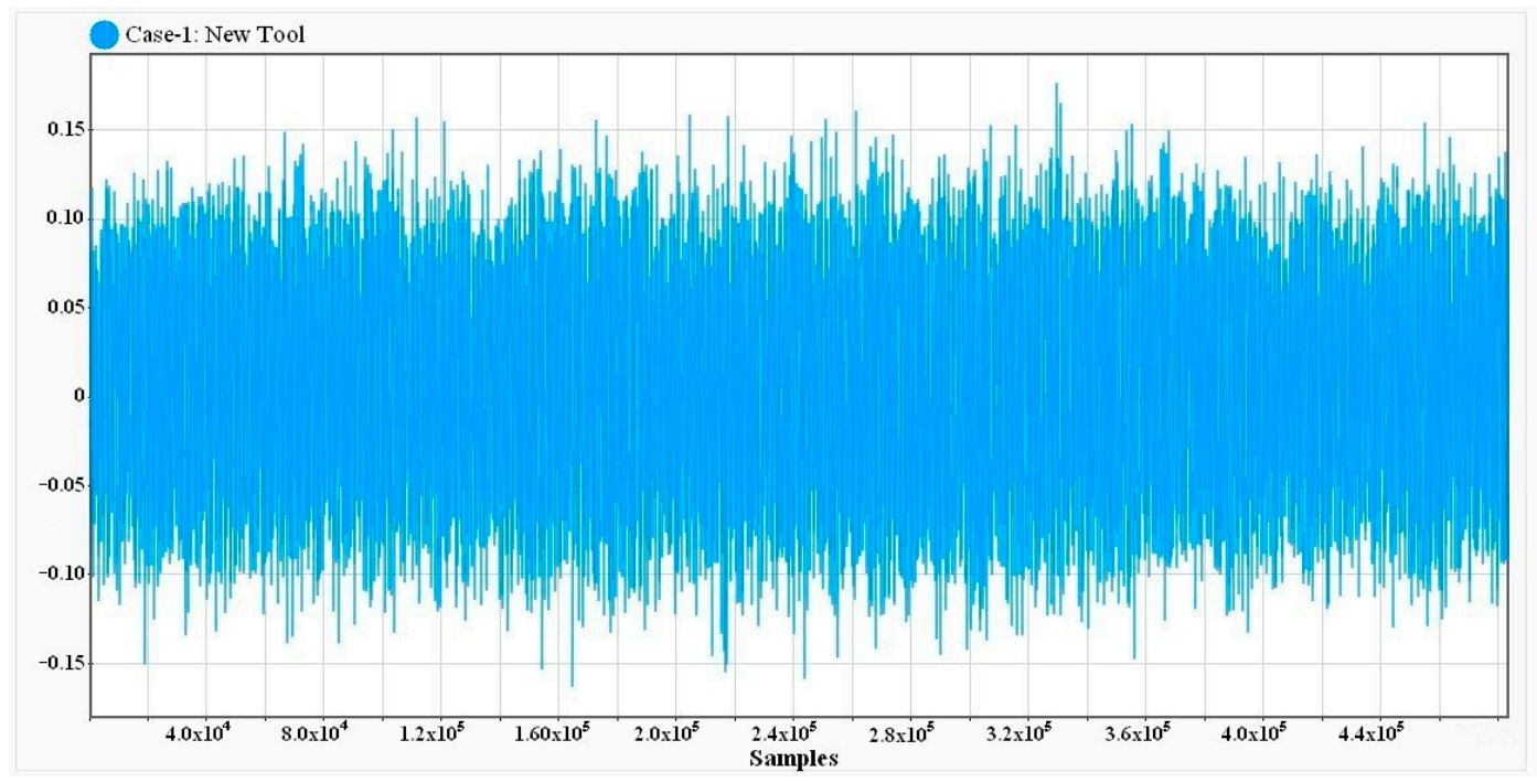
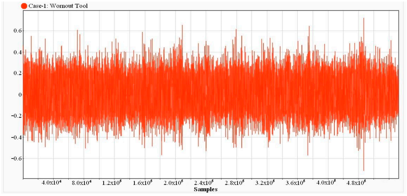
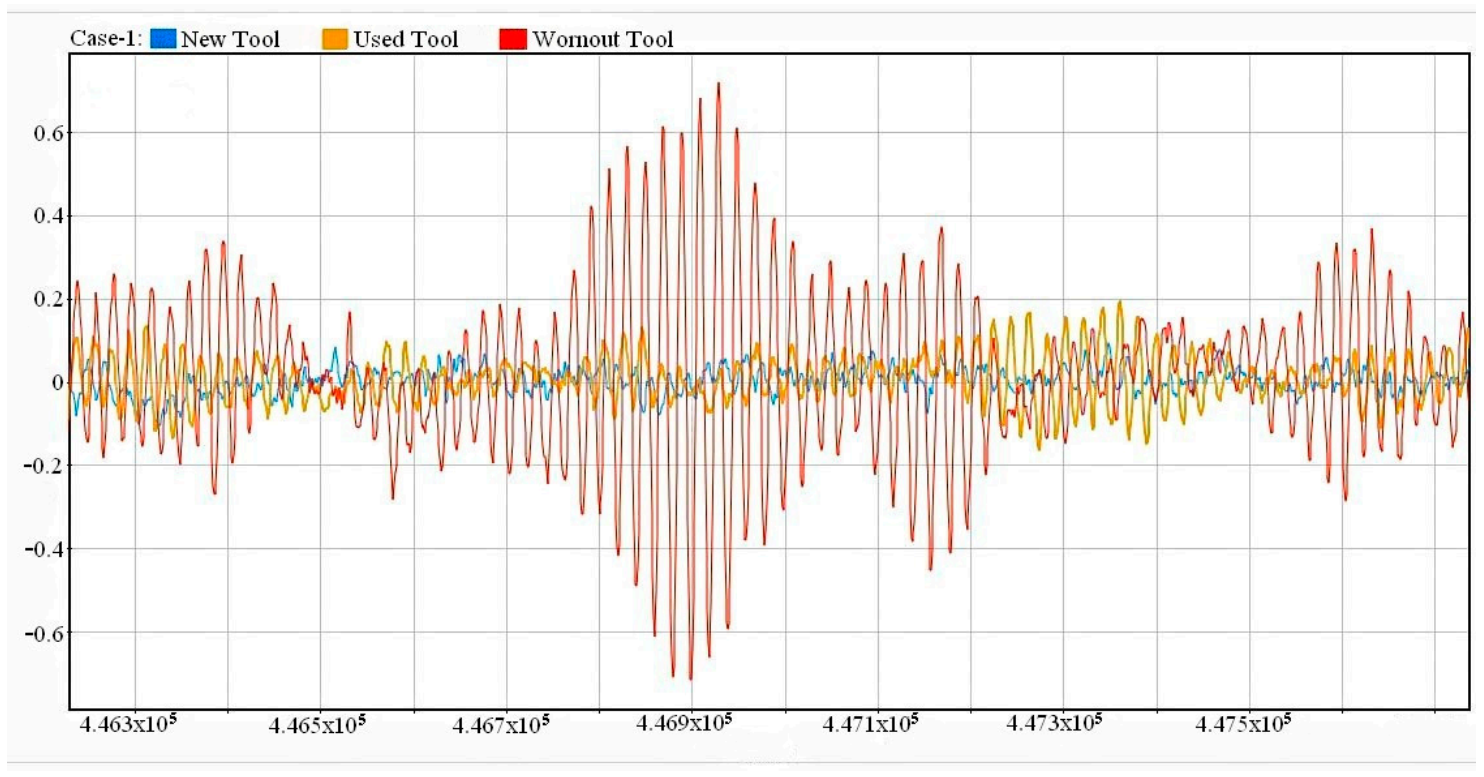
Airborne acoustic emission signals were acquired due to them lying in the audible frequency range of 20 Hz to 20 kHz [26]. The advantage of the air-borne AE signal acquisition is that the experimental setup used was rich in relevant information yet economically cheap. The whole machining process was acquired on a single ordinary microphone with a sampling frequency of 44.1 kHz to meet the Nyquist criteria. Figure 11 illustrates the flow diagram of the preprocessing of the AE signal. Thirty recordings were taken for each class of new, used, and worn-out for all tools and materials, as discussed in the experimentation section. Each recording was of 10 s duration and was further segmented into 10 pieces using a MATLAB^® script. Furthermore, the segments were saved in a .mat file format containing the time-domain vector of 44,100 samples. In total, six cases were formed with all the combinations. Figure 12, Figure 13 and Figure 14 are the raw 10 s AE signal time-domain representations for new, used, and worn-out tool categories (without any preprocessing) for the aluminum job and carbide tool for Case-1, respectively. The amplitude difference could be observed in the figures. Figure 15 presents the amplitude contrast for Case-1. A short window comparison of a few milliseconds of 10 s signals is shown. The new tool with the blue wave has the minimum amplitude, yellow for the medium tool has moderate amplitude, and red has the highest amplitude, representing a worn-out tool signature.

4.3. Raw AE Signals Characteristics

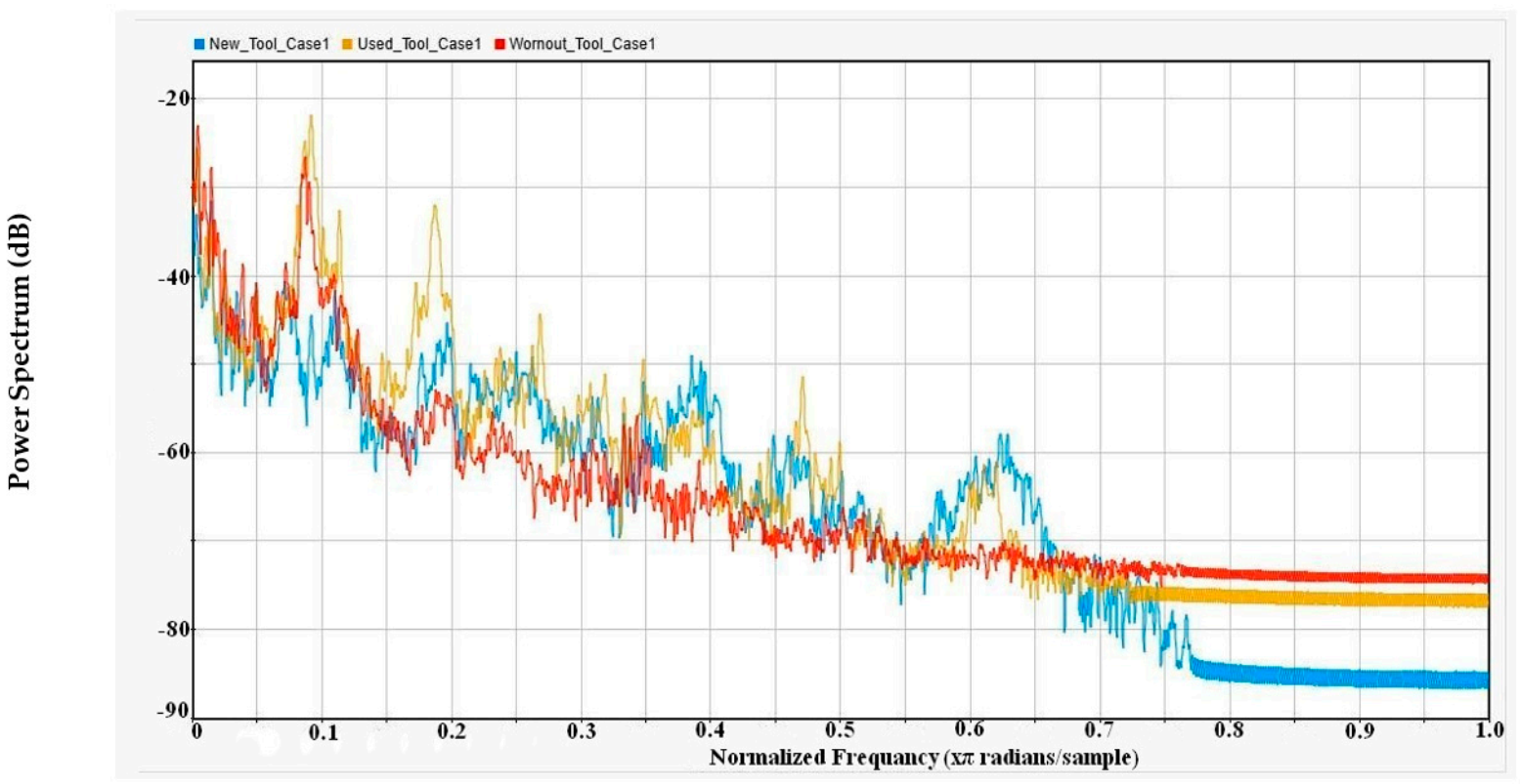
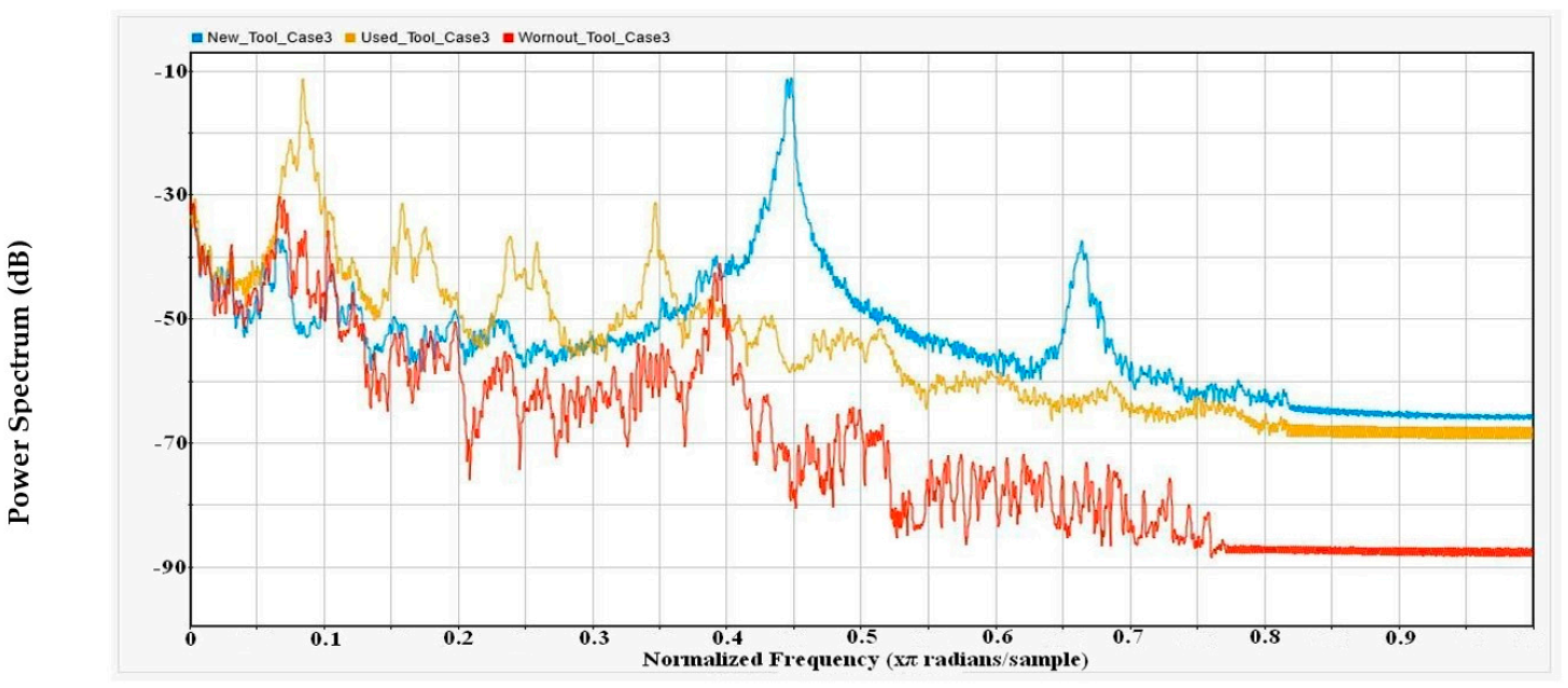
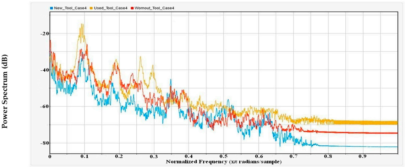
Power spectral density (PSD) is the averaged power of a signal in the frequency domain. PSD is a worthy illustrator of energy levels lying on the band of frequency showing which component of the frequency is outplaying in a particular signal. Figure 16, Figure 17, Figure 18, Figure 19, Figure 20 and Figure 21 are the normalized PSDs generated using the MATLAB^® Signal Analyzer application showing power levels on all frequency components for all cases. It is perceived that every case has a different PSD signature greatly dependent on the workpiece and tool type.

Raw acoustic signals in the time domain also contain useful statistical features that are distinct from each other, resulting in good classification practice [5,26,27]. Figure 22, Figure 23, Figure 24, Figure 25, Figure 26 and Figure 27 represent the six statistical features, RMS, mean, variance, skewness, kurtosis, and standard deviation, that have been calculated for the raw AE signal and are represented by bar graphs. Each figure represents the comparison of each statistical feature extracted for each case. Intuitively, frequency and time domain features failed to express promising trends or orders that are essential for attaining good training and classification for this experiment; there are no significant levels of unique or matching feature trend behaviors intra-categorically or inter-cases, respectively.

4.4. Visual Representation of Time–Frequency Domain: Spectrogram

In this research, a novel feature representation method is used that has never been addressed in the literature in this regard. A spectrogram is a visual demonstration of a signal that holds the capability of displaying three-dimensional information squeezed into a 2-dimensional data depiction such as time, frequency, and energy. In the experiment, after data acquisition and preprocessing steps, spectrograms have been acquired for all the AE data with the help of the MATLAB^® script, and then all the spectrogram images have been downsized to 500 × 500 size for standardization and faster algorithm processing speeds. Figure 22, Figure 23, Figure 24, Figure 25, Figure 26 and Figure 27 show the spectrograms for new, used, and worn-out tool categories for all six cases.

5. Classification Results

5.1. Convolutional Neural Network (CNN) Architecture

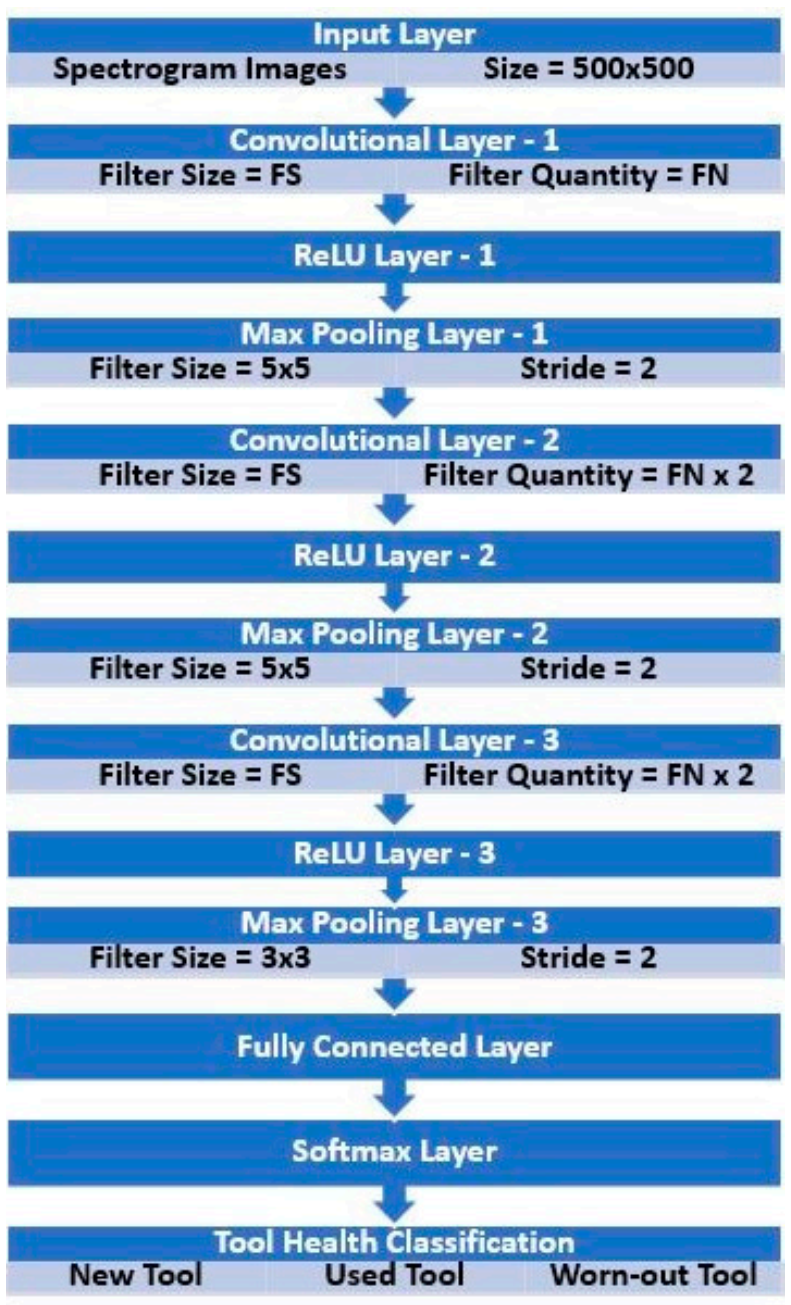
The convolutional neural network (CNN) technique is used for automatic feature extraction and classification using spectrogram images as input data. Figure 28 shows the complete single training scheme in which three layers of convolutions are used, followed by ReLU and pooling layers subsequently. A fully connected layer is used afterward to connect all the regions, as a result of the previous layers and finally after the softmax function implementation to attain the probabilities the classification results are attained in the classification layer.

5.2. Multiclass Quandary: Tool Health Classification

Tool health monitoring is realized as a three-class problem, which is also addressed as categories in this study, i.e., new, used, and worn-out tool categories. As discussed in the above sections, acoustic emissions for turning operation with six cases each containing these three categories were acquired at a 441,000 Hz sampling frequency of 10 s duration. These audio signals have been preprocessed on the later stage and window-sized at 44,100 to obtain a one-second duration AE signature. Three hundred single-second audio files were attained with this method for each category, and spectrograms were then developed from these AE signals. In total, 300 spectrogram images for each category have been made, forming 900 images for every case, and the whole experiment had 5400 spectrogram images in total including all six cases. Each case has been fed separately to the CNN classifier for the three-category-classification purpose. To attain the highest accuracies for all cases, the trained networks have been retrained on the trained weights, and then performance parameters were evaluated for both first-time-trained and retrained CNN networks. Performance parameters such as accuracy, specificity, sensitivity, and F1-score are standard and worthy performance evaluation criteria. The following performance parameters can be equated as:

$$Accuracy = \frac{TP+TN}{TP+TN+FP+FN}$$

(8)

$$Specificity = \frac{TN}{TN+FP}$$

(9)

$$Sensitivity = \frac{TP}{TP+FN}$$

(10)

$$F1-Score = 2\frac{\left(Precision\times Recall\right)}{\left(Precision+Recall\right)}$$

(11)

where TP and TN are true positive and true negative, respectively, while TN and FN are true negative and false negative, respectively. To access these parameters, a dataset has been prepared to be allocated into the training and testing dataset type. Seventy percent of the dataset is set for training and the remaining 30% dataset is subjected for testing and validation purposes. A promisingly consistent high-performance classification output for all cases is ensured after tuning the architecture through setting up different convolution filter sizes and the number of filters while the number of epochs were set to 10.

Table 2. Confusion matrix for case-1.

	Actual Class
	N = 900	New Tool	Used Tool	Worn-Out Tool
Predicted Class	New Tool	300	0	0
	Used Tool	0	300	0
	Worn-out Tool	0	0	300

shows the confusion matrix of the convolutional neural network applied on case-1, first training with four convolutional filters of 5 × 5 size. The matrix depicts that all three classes “new tool,” “used tool,” and “worn-out tool” have been learned and predicted correctly by the designed CNN architecture.

Table 3. Performance parameters for evaluation of CNN architecture for all cases of different number and sizes of filters including both trainings.

FS	FN		Case 1	Case 2	Case 3	Case 4	Case 5	Case 6	Average
5 × 5	4	Accuracy	1.000	0.980	0.998	0.988	0.988	0.998	0.992
		Precision	1.000	0.971	0.996	0.982	0.982	0.996	0.988
		Recall	1.000	0.970	0.996	0.981	0.981	0.996	0.987
		F1 Score	1.000	0.970	0.996	0.982	0.981	0.996	0.988
3 × 3	4	Accuracy	0.744	0.583	0.970	0.570	0.973	0.985	0.804
		Precision	0.818	0.464	0.959	0.319	0.962	0.979	0.750
		Recall	0.616	0.374	0.956	0.356	0.959	0.978	0.707
		F1 Score	0.527	0.277	0.955	0.221	0.959	0.978	0.653
10 × 10	4	Accuracy	0.556	0.852	0.556	0.575	0.840	0.556	0.656
		Precision	0.111	0.777	0.111	0.395	0.807	0.111	0.385
		Recall	0.333	0.778	0.333	0.363	0.759	0.333	0.483
		F1 Score	0.167	0.765	0.167	0.359	0.749	0.167	0.396
5 × 5	2	Accuracy	0.990	0.652	0.657	0.728	0.852	0.960	0.807
		Precision	0.986	0.480	0.741	0.792	0.790	0.949	0.790
		Recall	0.986	0.478	0.485	0.593	0.778	0.941	0.710
		F1 Score	0.986	0.431	0.428	0.584	0.776	0.940	0.691
5 × 5	6	Accuracy	1.000	0.988	0.837	0.686	0.556	0.960	0.838
		Precision	1.000	0.983	0.771	0.524	0.111	0.950	0.723
		Recall	1.000	0.983	0.756	0.530	0.333	0.941	0.757
		F1 Score	1.000	0.983	0.756	0.510	0.167	0.941	0.726

FS = Convolutional Filter Size, FN = Convolutional Number of Filters.

shows the resulting normalized performance parameters like accuracy, precision, recall, and F1-Score for all six cases that are accessed by tweaking the CNN network architecture with different sizes and number of filters. Another assessment has been done on the whole data set by retraining the trained weights and observing whether there has been any significant improvement in performance score benchmarks.

Results of the proposed technique outperformed the recent advance techniques added to the literature. Yu et al. [28] proposed a weighted hidden Markov model for CNC Milling tool health prediction, attaining an 81.64% accuracy in the best case. Luo et al. [29] used a deep learning model on the impulse response of tool vibration data to predict tool health, achieving a 98.1% accuracy at most, while the proposed technique has been able to have a consistent accuracy lying in between the range of 99% to 100% for all six cases using acoustic emission and convolutional neural network for CNC milling tool health monitoring.

6. Conclusions

This research proposed an acoustic emission and deep neural network architecture-based technique to detect the tool condition and to predict the tool health in real-time with accuracy using just a single acoustic emission sensor. Industry-oriented CNC turning operations were performed in the machine workshop on three different types of commercially utilized materials to predict the tool health on three different degradation adversity levels: “New,” “used,” and “worn-out” tools. Elastic waves generated during machining of the workpiece, and the resulting airborne acoustic emissions were recorded using a standard microphone, at a typical sampling rate of 44,100 Hz on a laptop, without any special treatment or exclusive signal acquisition procedure. Frequency and temporal domain features were analyzed individually, concluding that there were no reliable and unique categorical characteristics on which a robust tool health predictor could be formed. These one-dimensional AE signals are then preprocessed to represent time, frequency, and energy attributes in two-dimensional visual illustrations called spectrograms, which contained rich information about the AE signal. Convolutional neural network (CNN) architecture was developed, aimed to provide highly accurate tri-categorical tool health prediction. The spectrograms images were fed to the CNN directly as input without undergoing any extensive feature selection method. Different sizes and quantities of convolutional filters were used to determine the best combination, and two trainings were done for all six cases. The second training was the retraining with the learned weights from the first training. Four filters of 5 × 5 size gave consistently best accuracies for all the six cases while it was also observed that the retraining of the CNN produced significantly improved accuracies of 99% to 100% in all cases. In this experiment, the machining operation parameters have been set as constant for all six cases for the purpose of benchmarking, whereas the results of the experiment could be further improved by realizing the industry-standard machining parameters settings for every work-piece individually.

References

1. Manufacturing, Value Added (Current US$). Available online: data.worldbank.org/indicator/NV.IND.MANF.CD (accessed on 9 November 2020).
2. Manufacturing, Value Added (Annual % Growth). Available online: data.worldbank.org/indicator/NV.IND.MANF.KD.ZG (accessed on 9 November 2020).
3. Global and China CNC Machine Tool Industry Report, 2017–2021. December 2017. Available online: www.reportbuyer.com/product/4126834/global-and-china-cnc-machine-tool-industry-report-2017-2021.html (accessed on 9 November 2020).
4. Ray, N.; Worden, K.; Turner, S.; Villain-Chastre, J.P.; Cross, E.J. Tool wear prediction and damage detection in milling using hidden Markov models. In Proceedings of the International Conference on Noise and Vibration Engineering (ISMA), Leuven, Belgium, 19–21 September 2016. [Google Scholar]
5. Zhang, C.; Yao, X.; Zhang, J.; Jin, H. Tool Condition Monitoring and Remaining Useful Life Prognostic Based on a Wireless Sensor in Dry Milling Operations. Sensors 2016, 16, 795. [Google Scholar] [CrossRef] [PubMed] [Green Version]
6. Chen, X.; Li, B. Acoustic emission method for tool condition monitoring based on wavelet analysis. Int. J. Adv. Manuf. Technol. 2007, 33, 968. [Google Scholar] [CrossRef]
7. Dimia, D.E.; Lister, P.M.; Leighton, N.J. A multi-sensor integration method of signals in a metal cutting operation via application of multi-layer perceptron neural networks. In Proceedings of the Fifth International Conference on Artificial Neural Networks, Cambridge, UK, 7–9 July 1997. [Google Scholar]
8. Gao, H.; Xu, M.; Shi, X.; Huang, H. Tool Wear Monitoring Based on Localized Fuzzy Neural Networks for Turning Operation. In Proceedings of the 2009 Sixth International Conference on Fuzzy Systems and Knowledge Discovery, Tianjin, China, 14–16 August 2009. [Google Scholar]
9. Snr, D.E. Sensor signals for tool-wear monitoring in metal cutting operations—A review of methods. Int. J. Mach. Tools Manuf. 2000, 40, 1073–1098. [Google Scholar]
10. Li, X.L. A brief review: Acoustic emission method for tool wear monitoring during turning. Int. J. Mach. Tools Manuf. 2002, 42, 157–165. [Google Scholar] [CrossRef] [Green Version]
11. LeCun, Y.; Bottou, L.; Bengio, Y.; Haffner, P. Gradient-Based Learning Applied to Document Recognition. Proc. IEEE 1998, 86, 2278–2324. [Google Scholar] [CrossRef] [Green Version]
12. Kondrich, A. CS231n Convolutional Neural Networks for Visual Recognition. Available online: http://cs231n.github.io/convolutional-networks/#conv (accessed on 5 June 2017).
13. Simard, P.Y.; Steinkraus, D.; Platt, J.C. Best Practices for Convolutional Neural Networks Applied to Visual Document Analysis. In Proceedings of the Seventh International Conference on Document Analysis and Recognition (ICDAR 2003), Edinburgh, UK, 3–6 August 2003. [Google Scholar]
14. Zeiler, M.D.; Fergus, R. Visualizing and understanding convolutional networks. In European Conference on Computer Vision; Springer: Cham, Switzerland, 2014. [Google Scholar]
15. Simonyan, K.; Zisserman, A. Very deep convolutional networks for large-scale image recognition. arXiv 2014, arXiv:1409.1556. [Google Scholar]
16. Nair, V.; Hinton, G.E. Rectified linear units improve restricted Boltzmann machines. In Proceedings of the 27th International Conference on Machine Learning (ICML-10), Haifa, Israel, 21–24 June 2010. [Google Scholar]
17. Bishop, C.M. Pattern Recognition and Machine Learning; Springer: New York, NY, USA, 2016. [Google Scholar]
18. Murphy, K.P. Machine Learning: A Probabilistic Perspective; Adaptive Computation and Machine Learning; MIT Press: Cambridge, MA, USA, 2012. [Google Scholar]
19. Havelock, D.; Kuwano, S.; Vorländer, M. (Eds.) Handbook of Signal Processing in Acoustics; Springer: Berlin, Germany, 2008. [Google Scholar]
20. Abdelgawwad, A.; Catala, A.; Pätzold, M. Doppler Power Characteristics Obtained from Calibrated Channel State Information for Human Activity Recognition. In Proceedings of the 2020 IEEE 91st Vehicular Technology Conference (VTC2020-Spring), Antwerp, Belgium, 25–28 May 2020. [Google Scholar]
21. Sikdar, S.K.; Chen, M. Relationship between tool flank wear area and component forces in single point turning. J. Mater. Process. Technol. 2002, 128, 210–215. [Google Scholar] [CrossRef]
22. Malagi, R.R.; Rajesh, B.C. Factors influencing cutting forces in turning and development of software to estimate cutting forces in turning. Int. J. Eng. Innov. Technol. 2012, 2, 14–30. [Google Scholar]
23. Ayodeji, O.O.; Abolarin, M.S.; Yisa, J.J.; Olaoluwa, P.S.; Kehinde, A.C. Effect of Cutting Speed and Feed Rate on Tool Wear Rate and Surface Roughness in Lathe Turning Process. Int. J. Eng. Trends Technol. 2015, 22, 173–175. [Google Scholar]
24. Astakhov, V.P.; Davim, J.P. Tools (geometry and material) and tool wear. In Machining; Springer: London, UK, 2008; pp. 29–57. [Google Scholar]
25. Kumar, M.P.; Ramakrishna, N.; Amarnath, K.; Kumar, M.S.; Kumar, M.P.; Ramakrishna, N. Study on tool life and its failure mechanisms. Int. J. Innov. Res. Sci. Technol. 2015, 2, 126–131. [Google Scholar]
26. Zafar, T.; Kamal, K.; Sheikh, Z.; Mathavan, S.; Jehanghir, A.; Ali, U. Tool health monitoring for wood milling process using airborne acoustic emission. In Proceedings of the 2015 IEEE International Conference on Automation Science and Engineering (CASE), Gothenburg, Sweden, 24–28 August 2015. [Google Scholar]
27. Arslan, H.; Er, A.O.; Orhan, S.; Aslan, E. Tool condition monitoring in turning using statistical parameters of vibration signal. Int. J. Acoust. Vib. 2016, 21, 371–378. [Google Scholar] [CrossRef]
28. Yu, J.; Liang, S.; Tang, D.; Liu, H. A weighted hidden Markov model approach for continuous-state tool wear monitoring and tool life prediction. Int. J. Adv. Manuf. Technol. 2017, 91, 201–211. [Google Scholar] [CrossRef]
29. Luo, B.; Wang, H.; Liu, H.; Li, B.; Peng, F. Early Fault Detection of Machine Tools Based on Deep Learning and Dynamic Identification. IEEE Trans. Ind. Electron. 2018, 66, 509–518. [Google Scholar] [CrossRef]
Figure 1. Flow chart of the proposed technique.
Applsci 11 02734 g001
Figure 2. (Left) A typical neural network showing the interconnection of weights among all layers. (Right) Convolutional neural network (CNN) architecture with different layers with locally interconnected 3-dimensional weights [12].
Applsci 11 02734 g002
Figure 3. The first layer of the CNN is shown with the 3-dimensional input image (red), filter (yellow), activation map (blue), and five neurons activation (stacked in-depth dimension for the same region of filter convolution (yellow) with the input image) resulting from five filters of the corresponding colors (yellow, green, pink, purple, and brown) [12].
Applsci 11 02734 g003
Figure 4. Input layer with several slices has been downsampled after pooling to reduce parameters and avoid overfitting [12].
Applsci 11 02734 g004
Figure 5. Spectrogram generation from time-domain signal [19].
Applsci 11 02734 g005
Figure 6. Visual description of experiment group showing all six cases with work-pieces represented by blue boxes and tooltips and their categorization by white boxes.
Applsci 11 02734 g006
Figure 7. (Left) View of the whole experimental setup for computer numeric control (CNC) turning operation and data acquisition. (Right) Zoomed view of the setup illustrating the details of orientations.
Applsci 11 02734 g007
Figure 8. Workpieces of all three types on which turning operations have been performed.
Applsci 11 02734 g008
Figure 9. All three categories of carbide tool are shown where the level of tool degradation can be observed on each tooltip.
Applsci 11 02734 g009
Figure 10. All three categories of high-speed steel (HSS) tool are shown where the level of tool degradation can be observed on each tooltip.
Applsci 11 02734 g010
Figure 11. Flow diagram of data acquisition and preprocessing.
Applsci 11 02734 g011
Figure 12. Plot of raw acoustic emission (AE) signal of 10 s duration for new carbide tool on aluminum work-piece (Case-1).
Applsci 11 02734 g012
Figure 13. Plot of raw AE signal of 10 s duration for used carbide tool on aluminum work-piece (Case-1).
Applsci 11 02734 g013
Figure 14. Plot of raw AE signal of 10 s duration for worn-out carbide tool on aluminum work-piece (Case-1).
Applsci 11 02734 g014
Figure 15. Amplitude comparison of all three categories for Case-1 with new (blue), used (yellow) and worn-out (red) tools are shown.
Applsci 11 02734 g015
Figure 16. Power spectral density (PSD) for Case-1 of new (blue), used (yellow), and worn-out (red) tool with maximum leakage settings.
Applsci 11 02734 g016
Figure 17. Power spectral density (PSD) for Case-2 of new (blue), used (yellow), and worn-out (red) tool with maximum leakage settings.
Applsci 11 02734 g017
Figure 18. Power spectral density (PSD) for Case-3 of new (blue), used (yellow), and worn-out (red) tool with maximum leakage settings.
Applsci 11 02734 g018
Figure 19. Power spectral density (PSD) for Case-4 of new (blue), used (yellow), and worn-out (red) tool with maximum leakage settings.
Applsci 11 02734 g019
Figure 20. Power spectral density (PSD) for Case-5 of new (blue), used (yellow), and worn-out (red) tool with maximum leakage settings.
Applsci 11 02734 g020
Figure 21. Power spectral density (PSD) for Case-6 of new (blue), used (yellow), and worn-out (red) tool with maximum leakage settings.
Applsci 11 02734 g021
Figure 22. Spectrograms (training samples) of new, used, and worn-out tool conditions for Case 1.
Applsci 11 02734 g022
Figure 23. Spectrograms (training samples) of new, used, and worn-out tool conditions for Case 2.
Applsci 11 02734 g023
Figure 24. Spectrograms (training samples) of new, used, and worn-out tool conditions for Case 3.
Applsci 11 02734 g024
Figure 25. Spectrograms (training samples) of new, used, and worn-out tool conditions for Case 4.
Applsci 11 02734 g025
Figure 26. Spectrograms (training samples) of new, used, and worn-out tool conditions for Case 5.
Applsci 11 02734 g026
Figure 27. Spectrograms (training samples) of new, used, and worn-out tool conditions for Case 6.
Applsci 11 02734 g027
Figure 28. CNN architecture with layers sequence where FS = convolutional filter size, FN = number of convolutional filters.
Applsci 11 02734 g028