Abstract
A global geodetic reference system (GGRS) is realized by physical points on the Earth’s surface and is referred to as a global geodetic reference frame (GGRF). The GGRF is derived by combining several space geodetic techniques, and the reference points of these techniques are the physical points of such a realization. Due to the weak physical connection between the space geodetic techniques, so-called local ties are introduced to the combination procedure. A local tie is the spatial vector defined between the reference points of two space geodetic techniques. It is derivable by local measurements at multitechnique stations, which operate more than one space geodetic technique. Local ties are a crucial component within the intertechnique combination; therefore, erroneous or outdated vectors affect the global results. In order to reach the ambitious accuracy goal of 1 mm for a global position, the global geodetic observing system (GGOS) aims for strategies to improve local ties, and, thus, the reference point determination procedures. In this contribution, close range photogrammetry is applied for the first time to determine the reference point of a laser telescope used for satellite laser ranging (SLR) at Geodetic Observatory Wettzell (GOW). A measurement campaign using various configurations was performed at the Satellite Observing System Wettzell (SOS-W) to evaluate the achievable accuracy and the measurement effort. The bias of the estimates were studied using an unscented transformation. Biases occur if nonlinear functions are replaced and are solved by linear substitute problems. Moreover, the influence of the chosen stochastic model onto the estimates is studied by means of various dispersion matrices of the observations. It is shown that the resulting standard deviations are two to three times overestimated if stochastic dependencies are neglected.
1. Introduction
To get a better understanding of the dynamic processes on Earth, the global geodetic observing system aims for a global geodetic reference frame, which yields an accuracy of 1 mm for positions and a temporal stability of mm [1]. These accuracy requirements are essential for the global analysis of sea level rise, which is a direct effect of global warming [2]. Current realizations of a GGRS do not meet these requirements and are worse by a factor of 5 to 10 [3]. A GGRF is derived by combining several space geodetic techniques such as very long baseline interferometry (VLBI), satellite laser ranging, Doppler orbitography and radiopositioning integrated by satellite (DORIS), and the global navigation satellite system (GNSS) [4]. The physical points at the Earth’s surface, which realize the frame, are the reference points of these techniques. The most accurate realization is known as the International Terrestrial Reference Frame (ITRF), where the latest realization is denoted by ITRF2014 [5].
Due to the weak physical connection between the space geodetic techniques, further information that ties these techniques is necessary to derive a reliable frame. In this respect, so-called local ties are introduced to the combination procedure [6]. A local tie is the spatial vector defined between the reference points of two space geodetic techniques. It can be derived by local measurements at multitechnique stations, which host at least two different space geodetic techniques. Local ties provide the crucial component to overcome the weak physical connection between the space geodetic techniques. The vectors integrate the space techniques to a uniform Earth observation sensor at multitechnique stations [7].
Local ties are identified as a critical component within the intertechnique combination [8]. For instance, Altamimi et al. [9] evaluated the local ties used for the ITRF2014 and identified discrepancies of more than 5 mm for about 50% of the local ties w.r.t. the global solution. Therefore, strategies must be developed to improve local ties and the reference point determination procedure to reach the 1 mm goal. The common procedure of local tie determination consists of three analysis steps: The determination of the reference points of the space geodetic techniques in a local reference frame, preparing the local ties and the related dispersion matrices, and the mandatory transformation of the local ties into the GGRF using, for instance, homologous points. The last two steps are independent of the measurement method used for reference point determination, and always have to be performed. Novel approaches are being developed in joint projects such as the current GeoMetre research project [10], to traceably transfer local ties to the global frame [11]. For that reason, we restrict ourselves to the important first analysis step in this investigation.
Satellite laser ranging is a space geodetic technique organized under the International Laser Ranging Service (ILRS), which contributes to the origin and the scale of the GGRF. This investigation focuses on the analysis procedure of the ILRS reference point determination in a local frame. By convention, this reference point is defined by the orthogonal projection of the elevation axis onto the azimuth axis [12]. Since close range photogrammetry has been verified to be a suitable method to detect changes of the reflector geometries of VLBI radio telescopes with submillimeter accuracy [13,14,15], close range photogrammetry is transferred to the ILRS reference point determination of an SLR telescope, in this contribution. To the best of our knowledge, this is the first time close range photogrammetry has been used to determine the ILRS reference point. For that reason, the possible benefit w.r.t. the achievable accuracy and the measurement effort is investigated. Moreover, the influence of the stochastic model onto the estimates is studied by means of various dispersion matrices of the observations. Since most of the functional relations of the analysis process are nonlinear, we also address the bias of the estimates, which arises if the nonlinear function is replaced and is solved by its linear substitute problem.
Section 2 concerns the mathematical approaches that are used for data analysis in Section 3. The bundle adjustment and the reference point determination model are described in detail in Section 2.1 and Section 2.2, respectively. Moreover, the spherical simplex unscented transformation (SSUT) is introduced in Section 2.3. The SSUT is designed to efficiently obtain an approximated second-order accuracy for the estimates and allows investigation of the bias. A measurement campaign was carried out at the Geodetic Observatory Wettzell in September 2020. Section 3 describes the measurements and the analysis procedure. In Section 3.1, the chosen measurement instrument and the measurement configuration at the SLR telescope, the Satellite Observing System Wettzell, is presented. The data analysis and the obtained results are discussed in Section 3.2. Finally, Section 4 concludes this investigation.
2. Mathematical Background
The analysis part can be subdivided into three parts, i.e., the bundle adjustment, the reference point determination, and the analysis of the bias of the estimates. Section 2.1 summarizes the adjustment process of the photogrammetric measurements concerning the bundle adjustment as the initializing analysis step. The bundle adjustment yields coordinates of the observed points and the related fully populated dispersion matrix. These adjustment results are treated as observations for the reference point determination, which is addressed in Section 2.2.
The collinearity equations of the bundle adjustment and the reference point determination model are nonlinear. By applying the first-order Taylor series approximation of the nonlinear problem, the results are generally biased, because the stochastic properties of the linear substitute problem cannot be passed to the nonlinear problem. In Section 2.3, the spherical simplex unscented transformation is introduced to evaluate if the truncated Taylor series expansion yields sufficient results.
2.1. Bundle Adjustment
The functional model of the bundle adjustment relates the planar image coordinates to the spatial object point coordinates using the well-known collinearity equations ([16] p. 354), i.e.,
where
The principal distance is c, and , are the coordinates of the principal point. The distortion parameters are denoted by , . This set of parameters is referred to as interior orientation parameters. The so-called exterior orientation parameters are the jth spatial position and orientation of the camera. The matrix
is an orthogonal rotation matrix, i.e., and , and describes the spatial rotational sequence from the image frame to the object frame ([16] p. 281).
The distortion parameters , compensate for the radial-symmetric lens distortion and the decentring distortion. Beside noncausality models, which compensate for the effects without specifying the physical causes, causal models are used in photogrammetric applications, which model effects due to physical interactions ([17] p. 505). The Brown [18,19] approach is a causal model frequently applied in close range photogrammetry and, therefore, is used in this investigation.
The radial-symmetric lens distortion is characterized by the polynomial function
which is proportionally applied to the coordinate components, i.e.,
where , , and are the polynomial coefficients, and denotes the ith radial distance [19]. The decentring distortion with parameters , is given by [18,19]
Moreover, further parameters and concerning the affinity and shear components of the image plane can be taken into account ([16] p. 179f), i.e.,
However, for modern cameras, such parameters are rarely significant and can be neglected without losing accuracy [20].
Substituting Equations (4)–(9) into Equation (1) yields the functional model of the bundle adjustment, where the total correction term reads ([16] p. 180)
The observations are the image coordinates, which are automatically detected and identified by modern software packages. The parameters to be estimated are the spatial coordinates of the object points and the exterior orientation parameters, i.e., the spatial coordinates and orientation parameters of each camera position. This set of parameters is enlarged, if the interior orientation parameters are not known sufficiently, and leads to a self-calibration model [19,21]. Since Equation (1) is nonlinear, appropriate approximation values are required to estimate the parameters in terms of a least-squares adjustment.
The observed image coordinates provide redundant information about the inner geometry of the spatial network but are insensitive in terms of the datum definition, i.e., the definition of the origin, the orientation and the scale of the frame of the object points to be estimated. The resulting normal equation matrix has a rank deficiency D; thus, further conditions are required. A common approach also used in this investigation is to introduce up to linearly independent condition equations, which do not affect the inner geometry of the network. As shown by Papo [22], such a condition is fulfilled if the estimated coordinates , , are aligned to their approximation values , , . The no-net-translation (NNT) conditions, which correspond to the origin of the frame, are obtained by
The no-net-rotation (NNR) conditions, which define the orientation of the frame, are given by
The no-net-scale (NNS) condition reads
These datum conditions have to be applied to at least three noncollinear object points, and a Gauß–Markov model (GMM) with constraints can be setup to estimate the unknown parameters ([17] p. 104f).
2.2. Reference Point Determination
Satellite laser ranging is a space geodetic technique organized under the International Laser Ranging Service [23]. An SLR telescope is swivel-mounted around two axes, the azimuth axis and the elevation axis, and measures the distances to satellites [4]. For this purpose, the telescope transmits a short laser pulse signal towards a satellite that is equipped with retro reflectors, cf. Figure 1. The reflected signal is received by the telescope. The distance d between the retro reflector and the reference point of the SLR telescope is derived by the observed traveling time and the speed of light , i.e.,
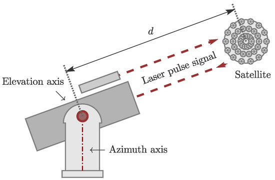
Figure 1.
Schematic representation of the satellite laser ranging (SLR) measurement principle.
For precise distance measurements, further corrections are applied to compensate for systematic errors, e.g., atmospheric errors or eccentricities of the telescope and satellite constructions ([24] p. 34ff).
The ILRS reference point of an SLR telescope is defined as the intersection point of the telescope axes. If both axes do not intersect, the point onto the azimuth axis, which is closest to the elevation axis, is the reference point [12]. Such a defined point is independent of the telescope orientation and is often referred to as invariant reference point (IRP). If this IRP is known w.r.t. to a reference point of a further space geodetic technique, both techniques become combinable within the intertechnique combination.
It is rather an exception that the IRP has been materialized and is observable by means of direct measurements. Usually, mounted markers at the turnable part of the telescope are observed in several telescope orientations. Based on the observed trajectories of these points, the IRP can be derived by means of geometric or transformation approaches. Geometric approaches derive the reference point by separating the trajectories into geometric primitives like spheres, circles, or tori. These approaches are simple and intuitive but have some disadvantages, e.g., a limited number of parameters or metrological restrictions. Transformation approaches overcome these disadvantages and determine the reference point by parameterizing the resulting trajectories of the mounted markers. The basic model reads [25]
and describes the functional relation of the point in a telescope fixed frame and its corresponding position in an Earth-fixed frame, e.g., the station network. Matrices are basic rotations around the subindexed coordinate axis using the braced angle. The index k denotes the orientation of the telescope at the measurement time. The angles and are the azimuth angle and the elevation angle, respectively. The axis offset is given by . The angles , parametrize the tilt of the azimuth axis w.r.t. the Z-axis of the Earth-fixed frame, and compensates for the deviation from the orthogonality of the two telescope axes. The translation vector corresponds to the IRP. Figure 2 depicts a schematic representation of the IRP transformation model.
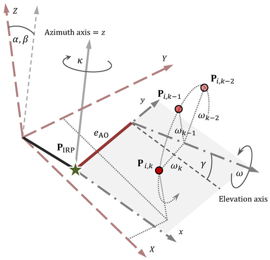
Figure 2.
Invariant reference point (IRP) transformation model that combines the grey dash-dotted depicted telescope fixed frame and the light red dashed depicted Earth-fixed reference frame. An arbitrary marker is shown in several k telescope orientations. The green star marks the reference point .
The observations in Equation (18) are the object coordinates that define the trajectories of . The parameters of the right-hand side are parameters to be estimated. Thus, the coordinates of are indicated as an explicit function of the unknowns, and a Gauß–Markov model can be used to estimate the parameters. However, as shown by Lösler et al. [26], the resulting normal equation matrix is rank-deficient, because the observed object coordinates are insensitive to define the orientation of the telescope frame. The rank deficiency becomes , if the trajectories of at least two markers are observed, and concerns the rotation around the elevation axis with angle . The problem is similar to the free adjustment discussed in Section 2.1, and the remaining rank deficiency can be solved by introducing the NNR condition
This condition is equivalent to Equation (14) and solves the rotation deficiency concerning the rotation around the x-axis of the telescope frame. Here, , are the approximation values of , and , are the estimated corrections. A detailed derivation of the reference point determination model and possible alternative datum conditions are discussed by Lösler et al. [26,27].
2.3. Spherical Simplex Unscented Transformation
Both the functional model of the bundle adjustment described in Section 2.1 and the functional model of the reference point determination model given in Section 2.2 are nonlinear. In these cases, the observations can be expressed as a function of the unknown parameters , which motivates the use of the nonlinear Gauß–Markov model.
Let the estimated correction of the unknown parameters w.r.t. the approximation values , the so-called reduced observation vector, the Jacobian matrix that contains the partial derivations of the linearized function w.r.t. , and vector be the normally distributed observational errors. Matrix is the known positive-definite dispersion matrix, also denoted as the stochastic model. The solution of the nonlinear problem is derived using the first-order truncated Taylor series of as a linear substitute problem within the GMM, i.e.,
Substituting and yields
and the well-known property of the expectation value of linear function is obtained, i.e.,
Here, tilde indicates true values.
However, introducing the second-order truncated Taylor series of as substitute problem yields
and the expectation value reads
where is the Hessian of the ith function in evaluated at [28,29,30]. For that reason, the linear substitute problem in Equation (20) is generally biased, if is nonlinear, and Equation (24) provides a second-order correction term. Analogically, one finds the expectation value for the dispersion [28,29,30], i.e.,
where the first term corresponds to the well-known linear propagation of errors, and the second term is the second-order correction of the dispersion.
The use of the second or higher-order Taylor series expansion becomes challenging, if the nonlinear function of the application results from a multidimensional and complex analysis procedure, such as for the bundle adjustment and the reference point determination. To evaluate the influence of the nonlinear function onto the estimates, usually a Monte Carlo simulation (MCS) is alternatively applied ([16] p. 654ff). In contrast to the truncated Taylor series, which approximates the nonlinear problem by a simplified substitute problem, the MCS approximates the probability distribution [31]. The MCS imitates a random experiment, e.g., a complex measurement process, using a large number of synthetically drawn pseudo-random numbers. The parameters and the dispersion are derived from numerical integration and, thus, are obtained by the equations for discrete random variables, i.e.,
The expectation values are asymptotically correct, if . Here, represents the ith randomly drawn sample, and , , denotes the corresponding weighting parameter, taken from the probability mass function ([32] p. 86ff). Since each randomly drawn experiment has the same probability, the weights are set to .
The disadvantage of the MCS is the large sample size, which is needed to approximate the probability distribution of the observations sufficiently. Especially in laser scanner applications, but also in close range photogrammetry projects, tens of thousands of observations are obtained, and the computational costs of the MCS increase dramatically, if the number of observations gets large.
As shown by Julier and Uhlmann [33] the number of synthetically drawn random samples can be reduced to a small set of deterministically derived neuralgic points, if a second-order bias corrected approximation is sufficient. The unscented transformation (UT) is such a method, and the standard UT is designed to obtain an approximated second-order accuracy for the parameters and the dispersion [34]. The neuralgic points , often referred to as -points, have the same first and second moment as the underlying sample and can be directly transformed using the nonlinear function [35], i.e.,
Inserting Equation (28) into Equations (26) and (27) yields a second-order approximation of the parameters and the dispersion, i.e.,
Meanwhile, there are several developed approaches within the UT framework. These approaches differ in the number of -points and in the procedure to generate the -points and the weights. A detailed survey of techniques is given by Menegaz et al. [36].
For real-time applications, Julier and Uhlmann [37] derive the minimal skew simplex unscented transformation (MSSUT), which only requires -points—the smallest possible number. However, this approach has a serious drawback, which limits the scope of applications. Due to the weights depending on via , these approach leads to numerical problems, even if the number of observations is moderate [38]. The spherical simplex unscented transformation (SSUT) avoids such numerical instabilities and is strongly recommended for large-scale problems ([39] p. 455f). According to Julier [38], the -points and the corresponding weights of the SSUT are derived by the following simple procedure ([40] p. 33):
- 1.
- Choose the weights as:
- 2.
- Set the vector sequence up according to:
- 3.
- Expand the vector sequence recursively for by:
- 4.
- Estimate the -points for as:
Here, is the square root of satisfying . The selected weight affects the fourth and higher-order moments of the -points [38]. For the number of -points is reduced to the minimum number of .
3. Satellite Observing System Wettzell
The Geodetic Observatory Wettzell is a GGOS core site and hosts instruments of all basic space geodetic techniques, including one DORIS beacon, three VLBI radio telescopes, two SLR laser telescopes, and several GNSS antennas [41]. Especially for this site, local tie vectors and reference point determination play an important role for the combination of space geodetic techniques to obtain a reliable and precise GGRF [42].
The use of alternative measurement techniques and analysis procedures is performed to figure out whether it improves the derived components or the measurement procedure. The following subsections describe the measurement configuration for the novel measurement approach using close range photogrammetry, and the key aspects of the analysis.
3.1. Measurements and Configurations
The measurement campaign for the evaluation of the potential of close range photogrammetry for reference point determination was carried out at GOW in September 2020. The investigations focus on the reference point determination of the Satellite Observing System Wettzell in a local frame. The SOS-W is the modern SLR laser telescope at GOW. It operates with a two-color laser for daytime and nighttime conditions to mainly reduce atmospheric refraction uncertainties [43]. The telescope is enclosed by a turnable protecting dome, comparable to a sphere with a diameter of about 5 and the telescope in its center, cf. Figure 3. A detailed description and the specifications of the laser telescope are given by Riepl et al. [44].
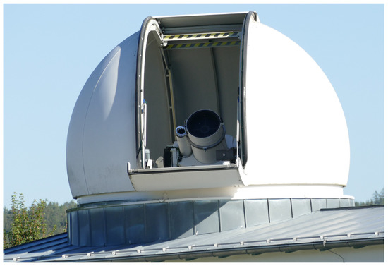
Figure 3.
Satellite Observing System Wettzell with turnable protecting dome at GOW.
Hexagon’s Aicon DPA Industrial measurement system is chosen for data acquisition and analysis, cf. Figure 4. The handheld digital camera-based photogrammetry system consists of the C1 camera, i.e., a Canon EOS 5D equipped with a 28 mm Aicon metric wide-angle lens that is protected by a robust and extremely stiff IP51-rated camera case, and the analysis software Aicon Studio 3D. The maximum permissible error (MPE) of a measured length, which is located between two signalized points, is specified by . The typical standard deviation of a position-based measurement obtained by a bundle adjustment, i.e., , is stated by [45]. Investigations on the geometric stability of the camera can be found in Rieke-Zapp et al. [46].
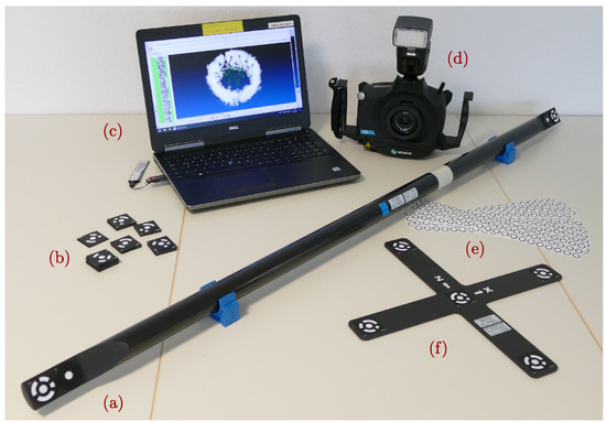
Figure 4.
Hexagon’s Aicon DPA Industrial measurement system consisting of the C1 camera (d) with a 28 mm metric lens, a coordinate-cross (f) for initial datum definition during the measurement process, scale bars (a) to trace to the SI meter, circular coded (b) and uncoded (e) photogrammetric markers, and the software package Aicon Studio 3D (c) for data analysis.
In this campaign, uncoded and 14-bit coded circular black-and-white markers are used. About 175 coded markers at the dome wall establish the photogrammetric reference frame. The frame is temporarily enlarged for the vertical component by further 50 coded markers beyond the wall of the dome. The scale information for the photogrammetric reference frame results from three calibrated scale bars, which are traced to the SI meter. The scale bars are located surrounding the telescope and contribute to all three coordinate components.
Nine interoperable drift nests (DN) are also mounted at the dome wall. They magnetically support reference markers for photogrammetric systems and corner cube reflectors for multilateration coordinate measurement systems [47] and for polar measurement systems such as laser trackers [26]. This interoperability of measurement systems is essential to combine different measurement techniques in a consistent reference frame, e.g., the station survey network. The drift nests can be embedded in the station survey network and ensure the integration of the results of the photogrammetric measurements. Thus, different measuring systems can be used for the reference point determination of each space geodetic technique and for the station survey network itself.
Kallio and Poutanen [48] evaluate the optimal position of mounted markers at the telescope structure by simulations and recommend marker positions close to the elevation axis. For that reason, uncoded photogrammetric markers are attached to the turnable part of the telescope. The maximum distance between the photogrammetric markers and the elevation axis is about 1 , and all markers are allocated at one side of the telescope balancing aspects of visibility, accessibility, and spatial coverage. Once the telescope is rotated to a different position, the markers are photogrammetrically observed. During the experiments, the telescope is rotated in equidistant steps for a homogeneous coverage of the working range of the SOS-W from 0° to 360° for the azimuth angle and 0° to 180° for the elevation angle. Figure 5 depicts the swivel-mounted laser telescope SOS-W in different elevation positions . The orange square symbolizes one of the photogrammetric markers , which is observed in several telescope orientations.
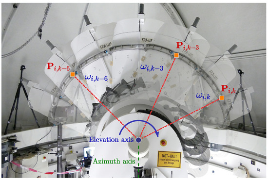
Figure 5.
Symbolic illustration of the swivel-mounted laser telescope SOS-W. The azimuth axis is represented by a green dotted line. The elevation axis is depicted by a blue dot. A mounted marker , symbolized by an orange square, is shown in several telescope orientations denoted by the elevation angle .
Table 1 summarizes the total number of analyzable images for the seven different experiments and the numbers of chosen azimuth and elevation positions. The number of images varies not only depending on the number of telescope positions, but also with the accessibility of favorable camera positions to achieve a wide range of different view angles. Each configuration is performed at least twice, so almost identical results can indicate their reliability. The horizontal distribution of the three different configurations is shown in Figure 6. The data presented in this study are available in the Supplementary Material.

Table 1.
Performed experiment configurations (Conf) w.r.t. to the number of telescope orientations in azimuth (Az) and elevation (El), the number of analyzable images (Img), and the effective number of marker positions n. The day of year (DOY) relates to 2020.
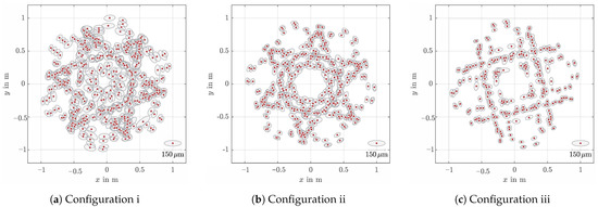
Figure 6.
Horizontal distribution of the resulting point clouds for the three measurement configurations having: (a) six
azimuths, seven elevations (i); (b) six azimuths, six elevations (ii); and (c) four azimuths, six elevations (iii). Grey ellipses
depict the 1s confidences derived by the fully populated dispersion of the bundle adjustment.
A single experiment takes between five and eight hours and is comparable to the common procedures for reference point determination using polar measurement instruments and only a few mounted markers [49,50]. In contrast to polar measurement systems, which sequentially observe the positions of mounted markers at the telescope, a single image of the photogrammetric measurement system captures several mounted markers simultaneously, and only a small number of images is needed to derive spatial coordinates. Thus, an increasing number of mounted markers does not significantly increase the number of images and the measurement effort.
3.2. Analysis and Results
The seven experiments of the measurement campaign given in Table 1 are individually analyzed to evaluate the influence of the different configurations onto the measurement results and to prove the repeatability of the estimates. The proprietary software package Aicon Studio 3D, which is part of the DPA measurement system, is used for preprocessing and analyzing the campaign. During a measurement experiment, the camera is connected to the software and transmits the captured images on the fly. Coded and uncoded black-and-white markers are automatically detected by pattern recognition ([16] p. 479ff) and image coordinates are derived. Moreover, approximation values of the exterior orientation parameters, i.e., the spatial coordinates and the orientation of each camera position, are estimated. Having the approximated exterior orientation parameters and the interior orientation parameters, which are approximately known from an external camera calibration, the image coordinates are transformed by Equation (1), and approximated spatial object point coordinates are obtained. As a result of these in-process preanalyses, approximation values for all required parameters are available.
Aicon Studio 3D package also provides a bundle adjustment module as described in Section 2.1. Beside the estimated parameters and the related standard deviations, parameters to evaluate the configuration and the reliability of the network are provided. However, the fully populated dispersion matrix of the estimated parameters, which is essential for a rigorous data analysis [51], is not provided [personal communication, Axel Kurze, 2018]. For that reason, the in-house software package JAiCov [52] was developed. The goal of the software is to readjust the final network based on the preanalysis results obtained by Aicon Studio 3D. JAiCov allows an independent verification of the adjustment results and provides the fully populated dispersion. Due to appropriate approximation values provided in a robust manner by Aicon Studio 3D, step-size control algorithms like damping, line search, or trust region approaches are currently not implemented. For numerical stabilization, the system of normal equations is preconditioned (cf. [53] p. 541ff).
3.2.1. Bundle Adjustment
The experiments of the measurement campaign are analysed individually as free-network adjustment, introducing NNT and NNR conditions to solve the rank deficiency of the normal equation matrix, cf. Equations (11)–(16). The NNS condition is omitted because three calibrated scale bars are observed, which are traced to the SI meter. The remaining datum conditions are exclusively applied to the nine DN points because these points are permanently marked, are interoperable with other measurement systems, and ensure the connection to the existing station network, cf. Section 3.1. According to Brown [19,21], distortion parameters of the camera are estimated within the bundle adjustment, which leads to the self-calibration approach described in Section 2.1.
Figure 6 depicts the horizontal distribution of the observed markers at the telescope for the three measurement configurations. Ellipses indicate the confidence level of the points obtained by the fully populated dispersion matrix of the bundle adjustment. Further global adjustment results are summarized in Table 2. The mounted markers have unique positions in the telescope fixed frame (object frame) but in the frame of the measurement instrument (reference frame) these markers yield trajectories. The number of observed positions per marker depends on the visibility of the marker and the number of different telescope orientations used during the experiment, cf. Table 1. For that reason, the number of unknowns as well as the number of observations increases, if the number of telescope orientations gets larger, see Figure 6. With one exception, all estimated are close to the expectation value and does not exceed 50 . For DOY 259, is slightly larger and exceeds its expectation value. The reason is not yet entirely clear and the effect is still under investigation. This configuration contains the smallest number of telescope orientations. However, DOY 260 uses an equivalent configuration but is inconspicuous. Thus, the reduction of telescope positions can be excluded as a possible cause.
Table 2.
Experiment-wise benchmark data of the bundle adjustments derived by JAiCov: and are the number of observations and unknowns, respectively. is the (unitless) variance of the unit weight. The mean standard deviations of the telescope points are given by , , , and . denotes the corresponding mean overall standard deviation of the bundle adjustment. Standard deviations are given in mm.
The mean standard deviations of the horizontal components and are comparable to each other but the vertical component is slightly smaller than the horizontal components. The reason is the distribution of the markers and the measurement configuration. Due to the geometry of the building, the markers mounted at the dome wall are cylindrically distributed around the telescope. This configuration yields a stiffer horizontal configuration but leads to a less controlled vertical component. In the horizontal plane, the camera positions surround the telescope, and the horizontal components are restrained by the cylindrical configuration. However, such a configuration can not be realized for the vertical component. For that reason, the standard deviation of the vertical component is slightly overestimated. To overcome this drawback, a spherical configuration of the markers that surrounds the object would be recommended. In practical applications, such an ideal configuration can not be realized due to building restrictions and environment obstructions.
As expected, the overall standard deviation of the bundle adjustment is slightly smaller than . Whereas the marker positions at the telescope are only observed for a dedicated time-span, i.e., for a specific telescope orientation k, the markers at the wall are repeatedly measured during the campaign. For that reason, the markers at the wall are more reliable, and occurs.
3.2.2. Reference Point Determination
The coordinates of the observed markers as well as the obtained fully populated dispersion matrix are treated as incomings for the reference point determination described in Section 2.2. Figure 7 depicts the variations of the estimated coordinate components of the reference point and the derived axis offset. Error-bars indicate the confidence level of the estimates. Corresponding numerical values are summarized in Table 3.
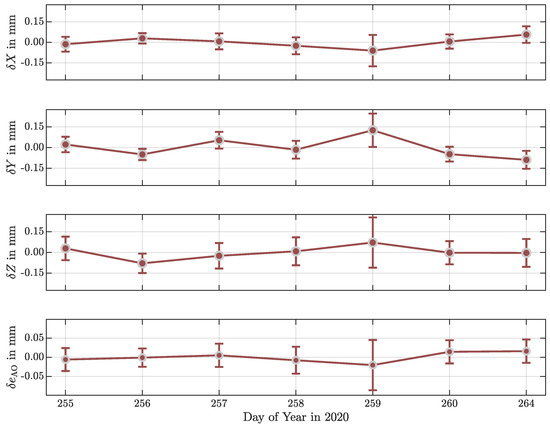
Figure 7.
Variations of the coordinate components of the reference point and the axis offset . Error bars indicate the confidence level.
Table 3.
Variations of the estimated reference point position , the derived axis offset , and the related standard deviations. All estimates are given in mm.
The coordinate components of the reference point and the axis offset vary in a range of about mm and mm, respectively. Moreover, the axis offset is close to zero and is insignificant. This result confirms prior investigations using a mobile laser tracker [26]. The derived standard deviations of the reference point coordinate components are comparable to the standard deviations of marker positions at the telescope. Values larger than mm are exceptions. Largest values can be found for DOY 259, which confirms the observed peculiarity during the bundle adjustment. The larger standard deviations of DOY 259 result from the uncertainty propagation, and are a direct consequence of the derived dispersion of the bundle adjustment, cf. Table 2. However, GGOS aims for an accuracy of 1 mm for the reference points and the local ties. This requirement contains the uncertainty budgeting of the reference point determination procedure, the local tie preparation, and the uncertainties of the transformation to the GGRF. As shown in Figure 7, close range photogrammetry allows for a reference point determination with superior accuracy. For comparison, the reported repeatability of a reference point determination using a total station is about ten times larger [49,54,55]. Therfore, the use of close range photogrammetry reduces the overall uncertainties significantly. The benefit of a dense point cloud, as it is realized by configuration i, does not significantly improve the estimates in comparison to the reduced configurations ii and iii but increases the measurement effort.
3.2.3. Bias of the Estimates
The functional model of the bundle adjustment given in Equation (1) and the reference point determination model in Equation (18) are nonlinear equations. By solving a linear substitute problem during the least-squares adjustment, the estimates are generally biased, cf. Equations (24) and (25). To estimate a second-order correction, the spherical simplex unscented transformation is applied as described in Section 2.3. Based on the observed image coordinates and , -points are generated according to Equation (37). By concatenating both nonlinear functional models, i.e.,
these -points are directly transformed. A second-order approximation of the reference point and the axis offset, and the related dispersion is obtained by Equations (29) and (30). Due to the large number of observations per measurement experiment, cf. Table 2, the SSUT is adopted once per configuration using the measurement experiments at DOY: 255, 258, 260.
Table 4 shows the differences between the second-order approximation derived by the SSUT and the linear substitute solution derived by the GMM. The differences of the estimated parameters are close to zero. Moreover, the derived standard deviations are biased by about 2 and 1 for the coordinates of the reference point and the axis offset, respectively.
Table 4.
Differences between the second-order approximation derived by the SSUT and the linear substitute solution derived by the GMM of the coordinates of the reference point , the axis offset , and the related standard deviations, i.e., . All estimates are given in .
In comparison to the variations depicted in Figure 7, the bias can be neglected. The reason can be found in Equations (24) and (25). The second-order correction consists of the Hessian matrix, obtained by the functional model, and the dispersion matrix, defining the stochastic model. Doubtlessly, the nonlinearity comes from the functional model, but the stochastic model controls the size of the bias onto the estimates [30,56]. Thanks to the high accuracy of close range photogrammetric systems but also due to the symmetric measurement configuration, the second-order effect becomes negligible, and the first-order solution yields proper estimates. This result confirms prior investigations using simulated data to evaluate reliable measurement configurations ([40] p. 86ff).
3.2.4. Impact of the Stochastic Model
The estimated parameters of a linear model are known to be unbiased, even if the stochastic model of the observation is misspecified ([57] p. 180). However, the dispersion of the estimated parameters is affected by an erroneous stochastic model [58]. To evaluate the impact of the chosen stochastic model onto the dispersion of the reference point and the axis offset, the fully populated dispersion matrix obtained by the bundle adjustment is replaced by four simplifications.
- 1.
- The most simplified stochastic model readswhich disregards all prior results derived by the bundle adjustment, i.e., the variances of the points and the dependencies between the points are neglected. Such a model is usually applied in curve and surface analyses [59,60]. Here, matrix is the identity matrix, and is the variance of the unit weight.
- 2.
- Using the variances given in yields the most common approach [61], because commercial software packages often provide the standard deviations , , and of the estimated object points. Having n points, this stochastic model readsLike before, all correlations are neglected.
- 3.
- Especially in laser scanning applications [61,62], a block-diagonal matrixis frequently used to define the stochastic model. The number of block matrices is equal to the number of observed points n, and the matrix is the ith symmetric block matrix that corresponds to the sub-matrix of the ith observed position in , i.e.,Here, , , and are the covariances between the coordinate components. Thus, correlations between the coordinate components of the point are taken into account, but correlations between the observed positions are still neglected.
- 4.
- The stochastic model, which takes the correlations between the observed positions realized by a single marker into account, is given bywhereis the symmetric block matrix of the lth mounted marker . The number of block matrices is equal to the number of mounted markers m. The resulting block-diagonal matrix neglects correlations between the positions obtained by different markers.
Figure 8 depicts the resulting standard deviations derived the by five different stochastic models and the three realized measurement configurations. The measurement configuration has only a minor effect on the estimated standard deviations, and all configurations under consideration yield comparable results. In contrast to the configuration, the chosen stochastic model affects the resulting standard deviations clearly. The results are similar for the simplified stochastic models , , and , and only differ by about 10%. These three models neglect most of the correlations in . In particular, the benefit of , which considers intrapoint correlations of , is quite small in comparison to the most simplified model . The block-diagonal matrix is more complex and considers intramarker correlations. The obtained standard deviations increase by about 40% and 10% for the reference point coordinates and the axis offset , respectively. However, introducing the fully populated dispersion matrix , which is by far the most complex stochastic model, yields the largest standard deviations. In comparison to the most simplified model , the resulting standard deviations derived by the fully populated dispersion matrix are three times and two times larger for the reference point coordinates and the axis offset , respectively. Neglecting the correlations between the observed positions overestimates the standard deviations, and overly optimistic results are obtained.
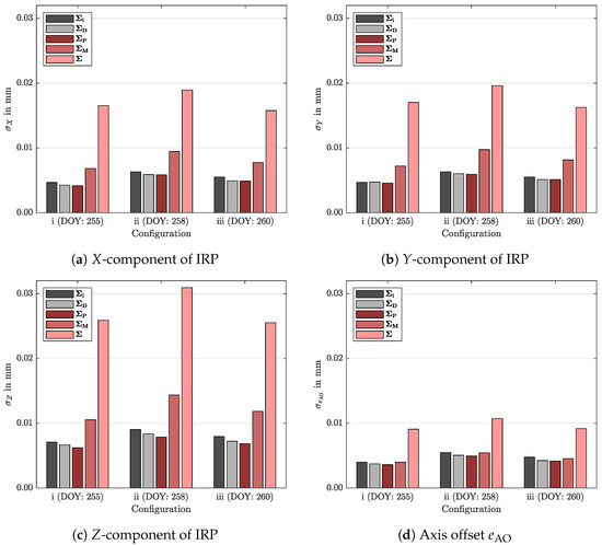
Figure 8.
Comparison of the resulting standard deviations of the coordinate components X, Y, Z of
the reference point and the axis offset eAO derived by three different measurement configurations,
denoted by i, ii, and iii, as well as five different stochastic models. The stochastic model defined by
the identity matrix, the diagonal matrix, and the block-diagonal matrix is denoted by ΣI (dark grey),
ΣD (light grey), ΣP (dark red), and ΣM (red), respectively. Σ (light red) indicates the stochastic model
introducing the fully populated dispersion.
The reason of the large differences depicted in Figure 8 is a consequence of the oversimplified stochastic models, which neglect most of the correlations. The frequency of the correlation coefficients derived by the correlation matrix
is depicted in Figure 9. Obviously, most of the parameters are positively correlated, cf. Figure 9a. About 88% of the correlation coefficients are in a range of about ±0.3. A second large accumulation is visible between 0.3 and 0.6, which contains about 10% of the coefficients. About 2% of the coefficients exceed 0.6 and indicate highly correlated parameters. The reason of this frequency is the structure of the correlation matrix . Figure 9b depicts the component-wise intracorrelation coefficients , , and , with , of an arbitrary marker position at the telescope, obtained from the ith row in . For the first 11 coefficients, the correlations exceed 0.7. Here, the corresponding coordinate components refer to positions of a dedicated telescope orientation defined by , . These coordinate components are highly correlated because they are observed (nearly) simultaneously by identical images. If the telescope orientation is changed, new coordinates are obtained for the mounted markers and the correlations strongly decrease. The intracorrelations of the horizontal coordinate components decrease below the 0.3-level. The average values excluding the first 11 coefficients are and for the x- and y-components, respectively. The correlations of the z-components remain higher and stagnate at about . The reason is the selected datum of the frame. Whereas the horizontal components of the mounted markers at the telescope are surrounded by the DN points, the vertical components of these points are located above the defined datum. Thus, the higher correlations of the vertical components indicate the dependencies between the chosen datum and the object points, and characterize the network extrapolation. These invaluable properties get neglected, if a simplified stochastic model is applied. To derive reliable and traceable results, it is highly recommended to introduce the fully populated dispersion to the analysis procedure.
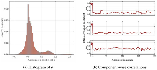
Figure 9.
Frequency of correlation coefficients for the observed positions, exemplified for DOY:
260. Whereas the histogram (a) contains the full set of correlation coefficients, in (b) componentwise
intracorrelations ρxixj, ρyiyj, and ρzizj of an arbitrary position are depicted. Self-correlations are
excluded in both figures.
4. Conclusions
Local tie vectors are one of the crucial components within the combination of space geodetic techniques for deriving a reliable reference frame. Such vectors are observable at multitechnique stations and are defined between the reference points of the hosted space geodetic techniques at the site. GGOS aims for a reference frame, which yields an accuracy of a global position of 1 mm. Current realizations do not meet these requirements and are worse by a factor of 5 to 10. One reason is the large discrepancy between the local ties and the global solution. To improve local ties and, thus, the reference points, suitable analysis procedures and measurement strategies must be developed.
In this investigation, close range photogrammetry is used for the first time to determine the ILRS reference point at the Satellite Observing System Wettzell in a local frame. For this purpose, a measurement campaign consisting of seven experiments using three different configurations was carried out in September 2020. The surrounding of the SOS-W was equipped with several coded and uncoded markers. The data were acquired and preprocessed using the photogrammetric system Aicon DPA Industrial. However, the proprietary software package Aicon Studio 3D does not provide the fully populated dispersion of the estimated object points. To overcome this drawback, the in-house software package JAiCov was developed, which obtains the dispersion of the final bundle adjustment. For each experiment, the marker positions and the related dispersion were introduced to the reference point determination process. The variations of the resulting coordinate components of the reference points are in a range of about mm w.r.t. the local datum. The axis offset varies of about and is insignificant. As shown in Figure 7, the benefit of a dense point cloud, as it was realized by configuration i, does not significantly improve the estimates in comparison to the reduced configurations ii and iii but increases the measurement effort significantly. Further investigations are needed to reduce the downtime of the telescope during the reference point determination. Procedures have to be developed to enable continues measurements during regular SLR experiments. In-process measurements allow for time series analysis to evaluate the repeatability and stability of the reference point.
Both the bundle adjustment described in Section 2.1 and the reference point determination model presented in Section 2.2 are nonlinear but are solved by transformed linear substitute problems within the GMM. Since stochastic properties of a linear substitute problem cannot be passed to the underlying nonlinear problem, the estimates are generally biased. By applying the spherical simplex unscented transformation to the analysis process, second-order improved results were obtained in this investigation. However, due to the high accuracy of the used close range photogrammetric system as well as the realized symmetric measurement configuration, the second-order effect becomes negligible. The first-order results derived by the GMM were proved to be proper.
The stochastic model was identified as the most crucial part of the analysis process, because it influences the dispersion of the reference point and the axis offset. Introducing a simplified stochastic model, i.e., a scaled identity matrix, a diagonal variance matrix, or a block diagonal matrix, yields an overestimated dispersion of the parameters. For instance, the standard deviations of the coordinate components of the reference point derived by the fully populated dispersion are about three times larger than for the most simplified model, cf. Figure 8. To avoid misinterpretations and to derive reliable and traceable results, it is highly recommended to introduce an appropriate stochastic model.
Supplementary Materials
The following are available online at https://www.mdpi.com/2076-3417/11/6/2785/s1.
Author Contributions
Conceptualization, M.L. and C.E.; methodology, M.L. and C.E.; analysis software, M.L.; remote control software, S.R.; formal analysis, M.L.; investigation, M.L. and C.E.; writing—original draft preparation, M.L., C.E., and T.K.; writing—review and editing, M.L., C.E., T.K., and S.R.; visualization, M.L.; project administration, C.E. and T.K. All authors have read and agreed to the published version of the manuscript.
Funding
This project 18SIB01 GeoMetre [10] has received funding from the EMPIR programme co-financed by the Participating States and from the European Union’s Horizon 2020 research and innovation programme.
Institutional Review Board Statement
Not applicable.
Informed Consent Statement
Not applicable.
Data Availability Statement
All data used in this paper are available in Supplementary Materials.
Conflicts of Interest
The authors declare no conflict of interest.
Abbreviations
The following abbreviations are used in this manuscript:
| DN | Drift nest |
| DORIS | Doppler orbitography and radiopositioning integrated by satellite |
| GGOS | Global geodetic observing system |
| GGRF | Global geodetic reference frame |
| GGRS | Global geodetic reference system |
| GMM | Gauß-Markov model |
| GNSS | Global navigation satellite system |
| GOW | Geodetic Observatory Wettzell |
| ILRS | International Laser Ranging Service |
| IRP | Invariant reference point |
| ITRF | International Terrestrial Reference Frame |
| MCS | Monte Carlo simulation |
| MPE | Maximum permissible error |
| MSSUT | Minimal skew simplex unscented transformation |
| NNR | No-net-rotation |
| NNS | No-net-scale |
| NNT | No-net-translation |
| UT | Unscented transformation |
| SLR | Satellite laser ranging |
| SOS-W | Satellite Observing System Wettzell |
| SSUT | Spherical simplex unscented transformation |
| VLBI | Very long baseline interferometry |
References
- Gross, R.; Beutler, G.; Plag, H.P. Integrated scientific and societal user requirements and functional specifications for the GGOS. In Global Geodetic Observing System—Meeting the Requirements of a Global Society on a Changing Planet in 2020; Plag, H.P., Pearlman, M., Eds.; Springer: Berlin/Heidelberg, Germany, 2009; pp. 209–224. [Google Scholar] [CrossRef]
- Blewitt, G.; Altamimi, Z.; Davis, J.; Gross, R.; Kuo, C.Y.; Lemoine, F.G.; Moore, A.W.; Neilan, R.E.; Plag, H.P.; Rothacher, M.; et al. Geodetic Observations and Global Reference Frame Contributions to Understanding Sea-Level Rise and Variability. In Understanding Sea-Level Rise and Variability; Church, J.A., Woodworth, P.L., Aarup, T., Wilson, W.S., Eds.; Wiley-Blackwell: Hoboken, NJ, USA, 2010; pp. 256–284. [Google Scholar] [CrossRef]
- Altamimi, Z.; Collilieux, X.; Boucher, C. Accuracy Assessment of the ITRF Datum Definition. In VI Hotine-Marussi Symposium on Theoretical and Computational Geodesy; Xu, P., Liu, J., Dermanis, A., Eds.; Springer: Berlin/Heidelberg, Germany, 2008; Volume 132, pp. 101–110. [Google Scholar] [CrossRef]
- Plag, H.P.; Altamimi, Z.; Bettadpur, S.; Beutler, G.; Beyerle, G.; Cazenave, A.; Crossley, D.; Donnellan, A.; Forsberg, R.; Gross, R.; et al. The goals, achievements, and tools of modern geodesy. In Global Geodetic Observing System—Meeting the Requirements of a Global Society on a Changing Planet in 2020; Plag, H.P., Pearlman, M., Eds.; Springer: Berlin/Heidelberg, Germany, 2009; pp. 15–88. [Google Scholar] [CrossRef]
- Altamimi, Z.; Rebischung, P.; Métivier, L.; Collilieux, X. ITRF2014: A new release of the International Terrestrial Reference Frame modeling nonlinear station motions. J. Geophys. Res. Solid Earth 2016, 121, 6109–6131. [Google Scholar] [CrossRef]
- Seitz, M.; Angermann, D.; Bloßfeld, M.; Drewes, H.; Gerstl, M. The 2008 DGFI realization of the ITRS: DTRF2008. J. Geod. 2012, 86, 1097–1123. [Google Scholar] [CrossRef]
- Schuh, H.; Wickert, J.; Sips, M.; Schöne, T.; Rogaß, C.; Roessner, S.; König, R.; Klemann, V.; Heinkelmann, R.; Dobslaw, H.; et al. Zukunft der globalen Geodäsie und Fernerkundung aus Sicht des Deutschen GeoForschungsZentrum (GFZ), Potsdam. In Handbuch der Geodäsie—Erdmessung und Satellitengeodäsie; Rummel, R., Ed.; Springer Reference Naturwissenschaften; Springer: Berlin/Heidelberg, Germany, 2017; pp. 443–497. [Google Scholar] [CrossRef]
- Glaser, S.; Fritsche, M.; Sośnica, K.; Rodríguez-Solano, C.J.; Wang, K.; Dach, R.; Hugentobler, U.; Rothacher, M.; Dietrich, R. Validation of Components of Local Ties. In REFAG 2014; van Dam, T., Ed.; Springer International Publishing: Cham, Switzerland, 2015; Volume 146, pp. 21–28. [Google Scholar] [CrossRef]
- Altamimi, Z.; Rebischung, P.; Métivier, L.; Collilieux, X. Analysis and Results of ITRF2014; IERS Technical Note 38, International Earth Rotation and Reference Systems Service (IERS); Verlag des Bundesamts für Kartographie und Geodäsie: Frankfurt am Main, Germany, 2017. [Google Scholar]
- GeoMetre. Large-Scale Dimensional Measurements for Geodesy—A Joint Research Project within the European Metrology Research Programme EMPIR; European Commission (EC), Grant Number: 18SIB01; EURAMET e.V.: Brunswick, Germany, 2020. [Google Scholar]
- García-Asenjo, L.; Baselga, S.; Atkins, C.; Garrigues, P. Development of a Submillimetric GNSS-Based Distance Meter for Length Metrology. Sensors 2021, 21, 1145. [Google Scholar] [CrossRef] [PubMed]
- Dawson, J.; Sarti, P.; Johnston, G.M.; Vittuari, L. Indirect approach to invariant point determination for SLR and VLBI systems: An assessment. J. Geod. 2006, 81, 433–441. [Google Scholar] [CrossRef]
- Kenefic, J.F. Ultra-Precise Analytics. Photogramm. Eng. 1971, 37, 1167–1187. [Google Scholar]
- Kim, H.; Yun, H.; Hwang, J.; Hong, S. A Static Displacement Monitoring System for VLBI Antenna Using Close-Range Photogrammetry. Appl. Sci. 2017, 7, 1125. [Google Scholar] [CrossRef]
- Lösler, M.; Haas, R.; Eschelbach, C.; Greiwe, A. Gravitational Deformation of Ring-Focus Antennas for VGOS–First Investigations at the Onsala Twin Telescopes Project. J. Geod. 2019, 93, 2069–2087. [Google Scholar] [CrossRef]
- Luhmann, T.; Robson, S.; Kyle, S.; Boehm, J. Close-Range Photogrammetry and 3D Imaging, 3rd ed.; Walter de Gruyter GmbH: Berlin, Germany, 2019. [Google Scholar] [CrossRef]
- Förstner, W.; Wrobel, B.P. Photogrammetric Computer Vision—Statistics, Geometry, Orientation and Reconstruction, 1st ed.; Geometry and Computing 11; Springer: Cham, Switzerland, 2016. [Google Scholar] [CrossRef]
- Brown, D.C. Decentering Distortion of Lenses. Photogramm. Eng. 1966, 32, 444–462. [Google Scholar]
- Brown, D.C. Close-Range Camera Calibration. Photogramm. Eng. 1971, 37, 855–866. [Google Scholar]
- Dai, F.; Feng, Y.; Hough, R. Photogrammetric error sources and impacts on modeling and surveying in construction engineering applications. Vis. Eng. 2014, 2, 2:1–2:14. [Google Scholar] [CrossRef]
- Brown, D.C. The Bundle Adjustment–Progress and Prospects. Int. Arch. Photogramm. 1976, 21, 1–33. [Google Scholar]
- Papo, H.B. Free Net Analysis in Close-Range Photogrammetry. Photogramm. Eng. Remote Sens. 1982, 48, 571–576. [Google Scholar]
- Pearlman, M.R.; Degnan, J.J.; Bosworth, J.M. The International Laser Ranging Service. Adv. Space Res. 2002, 30, 135–143. [Google Scholar] [CrossRef]
- Seitz, M. Kombination geodätischer Raumbeobachtungsverfahren zur Realisierung eines terrestrischen Referenzsystems. Ph.D. Thesis, Deutsche Geodätische Kommission, München, Germany, 2009. [Google Scholar]
- Lösler, M. New Mathematical Model for Reference Point Determination of an Azimuth-Elevation Type Radio Telescope. J. Surv. Eng. 2009, 135, 131–135. [Google Scholar] [CrossRef]
- Lösler, M.; Eschelbach, C.; Riepl, S. A Modified Approach for Automated Reference Point Determination of SLR and VLBI Telescopes. Tech. Mess. 2018, 85, 616–626. [Google Scholar] [CrossRef]
- Lösler, M.; Eschelbach, C.; Riepl, S.; Schüler, T. Zur Bestimmung des ILRS-Referenzpunktes am Satellite Observing System Wettzell. In Photogrammetrie-Laserscanning-Optische 3D-Messtechnik: Beiträge der 18. Oldenburger 3D-Tage 2019; Luhmann, T., Schumacher, C., Eds.; Wichmann Verlag: Oldenburg, Germany, 2019; pp. 162–175. [Google Scholar] [CrossRef]
- Box, M.J. Bias in Nonlinear Estimation. J. R. Stat. Soc. Ser. B 1971, 33, 171–201. [Google Scholar] [CrossRef]
- Teunissen, P.J.G. First and second moments of non-linear least-squares estimators. Bull. Géodésique 1989, 63, 253–262. [Google Scholar] [CrossRef][Green Version]
- Lösler, M.; Lehmann, R.; Neitzel, F.; Eschelbach, C. Bias in Least-Squares Adjustment of Implicit Functional Models. Surv. Rev. 2020, 1–12. [Google Scholar] [CrossRef]
- Julier, S.J.; Uhlmann, J.; Durrant-Whyte, H.F. A new method for the nonlinear transformation of means and covariances in filters and estimators. IEEE Trans. Autom. Control 2000, 45, 477–482. [Google Scholar] [CrossRef]
- Carlton, M.A.; Devore, J.L. Probability with Applications in Engineering, Science, and Technology, 2nd ed.; Springer Texts in Statistics; Springer International Publishing: Cham, Switzerland, 2017. [Google Scholar] [CrossRef]
- Julier, S.J.; Uhlmann, J.K. A Consistent, Debiased Method for Converting Between Polar and Cartesian Coordinate Systems. In Proceedings of the AeroSense: The 11th International Symposium on Aerospace/Defense Sensing, Simulation and Controls, Orlando, FL, USA, 21–25 April 1997; pp. 110–121. [Google Scholar] [CrossRef]
- Julier, S.J. The scaled unscented transformation. In Proceedings of the 2002 American Control Conference (IEEE Cat. No.CH37301), Anchorage, AK, USA, 8–10 May 2002; Volume 6, pp. 4555–4559. [Google Scholar] [CrossRef]
- Julier, S.J.; Uhlmann, J.K.; Durrant-Whyte, H.F. A new approach for filtering nonlinear systems. Proceedings of 1995 American Control Conference—ACC’95, Seattle, WA, USA, 21–23 June 1995; Volume 3, pp. 1628–1632. [Google Scholar] [CrossRef]
- Menegaz, H.M.T.; Ishihara, J.Y.; Borges, G.A.; Vargas, A.N. A Systematization of the Unscented Kalman Filter Theory. IEEE Trans. Autom. Control 2015, 60, 2583–2598. [Google Scholar] [CrossRef]
- Julier, S.J.; Uhlmann, J.K. Reduced sigma point filters for the propagation of means and covariances through nonlinear transformations. In Proceedings of the 2002 American Control Conference (IEEE Cat. No.CH37301), Anchorage, AK, USA, 8–10 May 2002; pp. 887–892. [Google Scholar] [CrossRef]
- Julier, S.J. The spherical simplex unscented transformation. In Proceedings of the 2003 American Control Conference, Denver, CO, USA, 4–6 June 2003; pp. 2430–2434. [Google Scholar] [CrossRef]
- Simon, D. Optimal State Estimation–Kalman, H∞, and Nonlinear Approaches; John Wiley & Sons, Inc.: Hoboken, NJ, USA, 2006. [Google Scholar] [CrossRef]
- Lösler, M. Modellbildungen zur Signalweg- und in-situ Referenzpunktbestimmung von VLBI-Radioteleskopen. Ph.D. Thesis, Technische Universität Berlin, Institute of Geodesy and Geoinformation Science, Geodesy and Adjustment Theory, Berlin, Germany, 2021. [Google Scholar] [CrossRef]
- Mähler, S.; Klügel, T.; Lösler, M.; Schüler, T. Permanentes Referenzpunkt-Monitoring der TWIN Radioteleskope am Geodätischen Observatorium Wettzell. Allg. Vermess. Nachrichten 2018, 125, 210–219. [Google Scholar]
- Rothacher, M.; Beutler, G.; Behrend, D.; Donnellan, A.; Hinderer, J.; Ma, C.; Noll, C.; Oberst, J.; Pearlman, M.; Plag, H.P.; et al. The Future Global Geodetic Observing System. In Global Geodetic Observing System—Meeting the Requirements of a Global Society on a Changing Planet in 2020; Plag, H.P., Pearlman, M., Eds.; Springer: Berlin/Heidelberg, Germany, 2009; pp. 237–272. [Google Scholar] [CrossRef]
- Riepl, S.; Müller, H.; Mähler, S.; Eckl, J.; Klügel, T.; Schreiber, U.; Schüler, T. Operating Two SLR Systems at the Geodetic Observatory Wettzell–From Local Survey to Space Ties. J. Geod. 2019, 8, 2379–2387. [Google Scholar] [CrossRef]
- Riepl, S.; Schlüter, W.; Dassing, R.; Haufe, K.H.; Brandl, N.; Lauber, P.; Neidhardt, A. SOS-W—A two colour kilohertz SLR system. In Proceedings of the 14th International Laser Ranging Workshop, Boletin ROA; Garate, J., Davila, J., Noll, C., Pearlman, M., Eds.; Ministerio De Defensa, Real Instituto y Observatorio de la Armada (ROA): San Fernando, Spain, 2005. Number 5. [Google Scholar]
- Hexagon. AICON DPA Series—Unrivalled High-End Photogrammetry Systems, Datasheet; Hexagon Manufacturing Intelligence: Brunswick, Germany, 2019. Available online: https://hexagonmi.com (accessed on 14 March 2021).
- Rieke-Zapp, D.H.; Tecklenburg, W.; Peipe, J.; Hastedt, H.; Haig, C. Evaluation of the geometric stability and the accuracy potential of digital cameras — Comparing mechanical stabilisation versus parameterisation. ISPRS J. Photogramm. Remote Sens. 2009, 64, 248–258. [Google Scholar] [CrossRef]
- Guillory, J.; Truong, D.; Wallerand, J.P. Uncertainty assessment of a prototype of multilateration coordinate measurement system. Precis. Eng. 2020. [Google Scholar] [CrossRef]
- Kallio, U.; Poutanen, M. Simulation of Local Tie Accuracy on VLBI Antennas. In Proceedings of the 6th IVS General Meeting 2010—VLBI2010: From Vision to Reality; NASA/CP-2010-215864. Behrend, D., Baver, K.D., Eds.; NASA: Greenbelt, MD, USA, 2010; pp. 360–364. [Google Scholar]
- Eschelbach, C.; Haas, R. The IVS-Reference Point at Onsala—High End Solution for a Real 3D-Determination. In Proceedings of the 16th European VLBI for Geodesy and Astrometry (EVGA) Working Meeting; Schwegmann, W., Thorandt, V., Eds.; Verlag des Bundesamtes für Kartographie und Geodäsie: Frankfurt am Main, Germany, 2003; pp. 109–118. [Google Scholar]
- Lösler, M. Reference point determination with a new mathematical model at the 20 m VLBI radio telescope in Wettzell. J. Appl. Geod. 2008, 2, 233–238. [Google Scholar] [CrossRef]
- Börlin, N.; Murtiyoso, A.; Grussenmeyer, P. Efficient Computation of Posterior Covariance in Bundle Adjustment in DBAT for Projects with Large Number of Object Points. In Proceedings of the XXIV ISPRS Congress, International Society for Photogrammetry and Remote Sensing, Virtual Event, Nice, France, 31 August–2 September 2020; pp. 737–744. [Google Scholar] [CrossRef]
- JAiCov. Java Aicon Covariance matrix—Bundle Adjustment for Close-Range Photogrammetry. 2021. Available online: https://github.com/applied-geodesy/bundle-adjustment (accessed on 14 March 2021).
- Schwarz, H.R.; Köckler, N. Numerische Mathematik, 8th ed.; Vieweg + Teubner Verlag, Springer Fachmedien: Wiesbaden, Germany, 2011. [Google Scholar] [CrossRef]
- Klügel, T.; Mähler, S.; Schade, C. Ground Survey and Local Ties at the Geodetic Observatory Wettzell. In Proceedings of the 17th International Workshop on Laser Ranging—Extending the Range; Schreiber, U., Pearlman, M., Appleby, G., Eds.; Verlag des Bundesamtes für Kartographie und Geodäsie: Frankfurt am Main, Germany, 2012; Volume 48, pp. 127–131. [Google Scholar]
- Lösler, M.; Haas, R.; Eschelbach, C. Automated and continual determination of radio telescope reference points with sub-mm accuracy: Results from a campaign at the Onsala Space Observatory. J. Geod. 2013, 87, 791–804. [Google Scholar] [CrossRef][Green Version]
- Lehmann, R.; Lösler, M. Hypothesis Testing in Non-Linear Models Exemplified by the Planar Coordinate Transformations. J. Geod. Sci. 2018, 8, 98–114. [Google Scholar] [CrossRef]
- Koch, K.R. Parameter Estimation and Hypothesis Testing in Linear Models; Springer: Berlin/Heidelberg, Germany, 1999. [Google Scholar] [CrossRef]
- Kutterer, H. On the sensitivity of the results of least-squares adjustments concerning the stochastic model. J. Geod. 1999, 73, 350–361. [Google Scholar] [CrossRef]
- Neitzel, F.; Ezhov, N.; Petrovic, S. Total Least Squares Spline Approximation. Mathematics 2019, 7, 462. [Google Scholar] [CrossRef]
- Lösler, M.; Eschelbach, C. Orthogonale Regression—Realität oder Isotropie? Tech. Mess. 2020, 87, 637–646. [Google Scholar] [CrossRef]
- Zhao, X.; Kermarrec, G.; Kargoll, B.; Alkhatib, H.; Neumann, I. Influence of the simplified stochastic model of TLS measurements on geometry-based deformation analysis. J. Appl. Geod. 2019, 13, 199–214. [Google Scholar] [CrossRef]
- Kermarrec, G.; Alkhatib, H.; Neumann, I. On the Sensitivity of the Parameters of the Intensity-Based Stochastic Model for Terrestrial Laser Scanner. Case Study: B-Spline Approximation. Sensors 2018, 18, 2964. [Google Scholar] [CrossRef] [PubMed]


Publisher’s Note: MDPI stays neutral with regard to jurisdictional claims in published maps and institutional affiliations. |
© 2021 by the authors. Licensee MDPI, Basel, Switzerland. This article is an open access article distributed under the terms and conditions of the Creative Commons Attribution (CC BY) license (http://creativecommons.org/licenses/by/4.0/).