Abstract
In this study, we propose a multi-scale ensemble learning method for thermal image enhancement in different image scale conditions based on convolutional neural networks. Incorporating the multiple scales of thermal images has been a tricky task so that methods have been individually trained and evaluated for each scale. However, this leads to the limitation that a network properly operates on a specific scale. To address this issue, a novel parallel architecture leveraging the confidence maps of multiple scales have been introduced to train a network that operates well in varying scale conditions. The experimental results show that our proposed method outperforms the conventional thermal image enhancement methods. The evaluation is presented both quantitatively and qualitatively.
1. Introduction
Many kinds of research have been conducted on how to obtain a thermal image of high quality, which is needed in a wide range of applications: face detection and tracking [], breast abnormality evaluation [], pipeline leak recognition [], and advanced driver assistance systems [,,]. Recently, due to the COVID-19 pandemic, the demand for thermal-based technologies, such as contactless body temperature acquisition, has been substantially increased [,,]. As the thermal images are robust to the dark illumination environment and also have the merit of containing the thermal information of an object, they have been playing an important role in addressing the limitations of visual sensors. Regardless of the level of illumination, mid- and long-wavelength infrared spectra are captured by thermal cameras and result in the temperature information. However, the hardware equipment for a thermal image of high quality is not only generally expensive, but also often massive. There is a trade-off either between the quality of a thermal image and the economical efficiency or between the quality of a thermal image and the practical usability.
Several approaches have been proposed to improve a low-quality thermal image by only leveraging software-based techniques. The approaches include detail enhancement (super-resolution) [,,,,,], noise reduction [,,,], contrast enhancement [,,,], etc.
Although public thermal datasets have been released [,,,,,,,], the authors in [,] found that training a network using visual images is more effective for improving a thermal image than training a network with thermal images themselves. They concluded that one should train the network using the visual domain to improve the quality of a thermal image, and these visual-based networks achieve better performance on the thermal image test datasets. This is because various and massive datasets are essential for the training procedure, and there are relatively much more visual datasets than thermal datasets. Nevertheless, Lee et al. [] suggested the possibility that the network trained based on a thermal dataset can show better performance provided that the size of the datasets is fairly comparable.
Still, recent thermal image enhancement methods based on deep learning networks, which are trained using images of a fixed scale [,,,], can only improve the quality of a thermal image for a certain image scale. For this reason, the performances of these networks degrade when applying different scales of low-quality images as the input.
To address this issue, we propose a multi-scale ensemble learning method for thermal image enhancement in varying scale conditions. Our network was designed as a novel parallel architecture leveraging the confidence maps of multiple levels. We designed our network with n-level parallel sub-networks to handle the images of different scales using a single network. Our network was newly constructed by building up individual sub-networks adopted from [], except that the dimension of an output in a reconstruction module was doubled because of the additional confidence map. Each sub-network was trained to predict a pair of a residual image and a confidence map. To strengthen the connectivity between sub-networks, a mixed feature module was added, which concatenates the feature maps of each sub-network, and the concatenated feature map by this module was also trained to predict a pair of those. Subsequently, a total of pairs of residual and confidence maps were combined using a combination module to produce a finally enhanced thermal image. The experimental results showed that the proposed network outperformed the state-of-the-art approaches in varying scale conditions with respect to the peak signal-to-noise ratio (PSNR) and structural similarity (SSIM) []. The remainder of this paper is organized as follows. Section 2 presents a review of the related works, and Section 3 describes the proposed network in detail. The experimental results and discussion are provided in Section 4. Finally, the conclusions are stated in Section 5.
2. Background
Thermal image enhancement can be largely categorized into three topics: detail enhancement (super-resolution), noise reduction, and contrast enhancement. Firstly, the detail enhancement of a thermal image is done to improve a low-quality thermal image and turn it into a high-quality one. Choi et al. [] suggested a convolutional neural network-based super-resolution approach. Through the comparison between networks using gray and midwave infrared images, they found that the network using gray images showed better performance than the one using midwave infrared images. In addition, they verified that the improvement in the quality of a thermal image led to the performance enhancement of the applications. Lee et al. [] presented a residual network for thermal image enhancement. They experimentally verified that the brightness domain is best suited for training a network for thermal image enhancement. This method generates a high-quality thermal image by element-wise summation of low-quality input and residual output images. Rivadeneira et al. [] introduced the networks trained by visual and thermal images that were based on []. They also released a public dataset that has 101 thermal images acquired using a TAU2 thermal camera. Gupta and Mitra [] proposed a hierarchical edge-based guided super-resolution method. This method needs visible-range images to extract multi-level edge information. Rivadeneira et al. [] suggested the CycleGAN-based [] super-resolution method. This method considers the scale factor ×2 in two different scenarios. The first scenario is to generate mid-resolution images from low-resolution images. Secondly, high-resolution images are generated from mid-resolution images. Furthermore, the authors released thermal datasets captured with three different devices for low-resolution, mid-resolution, and high-resolution thermal images. Cascarano et al. [] presented a super-resolution algorithm for aerial and terrestrial thermal images, which was based on total variation regularization. This method is a fully automatic method with a low-cost adaptive rule. In addition, they introduced a new thermal image quality metric based on a specific region of interest for radiometric analysis.
Then, to reduce the noise of a thermal image, Zeng et al. [] used spectral and spatial filters with a two-stage strategy. They analyzed the noise pattern and improved the level of stripe non-uniformity correction while preserving the details. Lee and Ro [] suggested a de-striping convolutional neural network based on a double-branched structure using a parametric noise model. The parametric fixed pattern noise model was built through diagnostic experiments of infrared images using the physical principle of the infrared detector and the signal response. The model parameters were optimized using measurement data collected over a wide range of detector temperatures. They also generated the training data using the models to ensure stable performance for various patterns.
Lastly, for the contrast enhancement of a thermal image, Ibrahim and Kong [] introduced the histogram equalization-based method. This method increases the global contrast by distributing the thermal histogram almost evenly. Bai et al. [] adopted a multi-scale top-hat transform. Kuang et al. [] presented a conditional generative adversarial network-based method trained on visible images. This approach has two elements, a generative sub-network and a conditional discriminative sub-network.
As mentioned above, various research topics have been studied, including detail enhancement, contrast enhancement, and noise reduction. Contrast enhancement is a method for improving the quality of an image considering that human visual perception is more sensitive to the changes in contrast than the changes in brightness. However, since this method is used to change the pixel value of the thermal image, that is the temperature value itself, it brings about a difficulty in implementing the changed values directly in some applications that use temperature values such as body temperature measurement. For detail enhancement, Choi et al. [] verified that the performance of pedestrian detection can be improved using enhanced thermal images by the convolutional neural network for super-resolution. For this reason, we also focus on detail enhancement to improve details while preserving temperature information as much as possible.
3. Proposed Network
In this section, we describe our approach for robust thermal image enhancement in varying scale conditions, which takes an input of the same size as the output. The proposed network is composed of n-level sub-networks, and each level contains three modules: feature extraction, mapping, and reconstruction through residual connection. The variables of a sub-network (the number of layers, kernel size, and feature channels) were set according to [] except for the doubled dimension of an output in the reconstruction module, as shown in Table 1. The dimension of an output in the reconstruction module was set to two by adding one more dimension for the confidence map. At each sub-network, a pair of a residual image and a confidence map is generated. Subsequently, the mixed feature module concatenates the output feature maps of all mapping modules and also generates a pair of residual image and confidence map using the following reconstruction module as shown in Table 2. Consequently, pairs of residual images and confidence maps are combined to predict the final high-quality thermal image, as illustrated in Figure 1. The details of the network are explained in the following subsections.

Table 1.
The configuration of the sub-networks.
Table 2.
The configurations of the mixed feature module and reconstruction module.
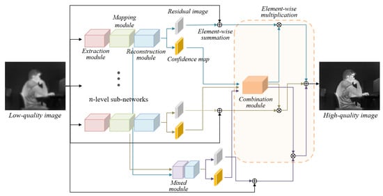
Figure 1.
The structure of our proposed network.
3.1. Sub-Network
Table 1 shows the configuration of the sub-network, which consists of feature extraction, mapping, and reconstruction modules.
3.1.1. Feature Extraction Module
This module extracts a set of feature maps from the input image (see Figure 2). It consists of a total of three layers. The first layer learns to generate 48 channels of the output feature map by taking an input image as a single channel. The following two layers receive the 48 channels of the feature map from the previous layer. Finally, an output feature map of the size of 48 channels is extracted. Each layer is a 3 × 3 kernel size convolutional layer, and we adopted PReLU [] for the activation function.
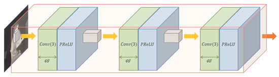
Figure 2.
Visualization of the feature extraction module.
3.1.2. Mapping Module
In this module, the feature maps from the feature extraction module are non-linearly mapped (see Figure 3). The first layer, namely shrinking, and the last layer, namely expansion, reduce and expand the number of channels of the feature map by a convolutional layer with a 1 × 1 kernel, respectively. Through these layers, the mapping module can be deeply constructed so that the non-linearity can be increased. The five middle layers, which are 3 × 3 kernel size convolutional layers, have 16 channels of feature maps for nonlinear mapping. PReLU is used as the activation function for all convolutional layers in this module.
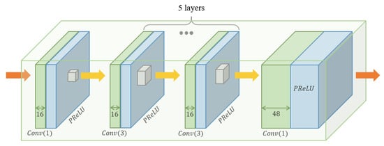
Figure 3.
Visualization of the mapping module.
3.1.3. Reconstruction Module
This module aggregates the feature maps and predicts information in two dimensions (see Figure 4). The first information is the residual image, and the second is the confidence of the pixel in an image, as shown in Figure 5. The reconstruction module is located both after the mapping module of each sub-network and after the mixed feature module. Therefore, there is a total of reconstruction modules in the proposed network. The convolutional layer in this module has a 3 × 3 kernel without any activation function.
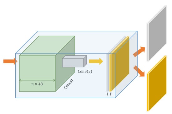
Figure 4.
Visualization of the reconstruction module.
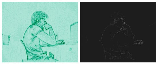
Figure 5.
An example of a pair of (left) a confidence map and (right) a residual image (normalized and color mapped to deep green and gray for visualization).
3.2. Mixed Feature Module
To improve the connectivity of the sub-networks, we concatenated the feature map of each level of the sub-network. The concatenated feature map of n × 48 channels is learned to predict an additional residual image and a confidence map using the reconstruction module, as shown in Table 2. Then, a total of pairs of residual images and confidence maps become available.
3.3. Combination Module
In this module, pairs of residual images and confidence maps are learned to finally produce a high-quality thermal image. The confidence maps are learned so that the values at a certain position sum up to one by using a softmax layer. That is, the confidence map of a sub-network indicates how much weight should be assigned to the sub-network when producing an output. Subsequently, the output image of each sub-network is element-wisely multiplied by its confidence map and then element-wisely summed to generate a high-quality thermal image as in Equations (1).
where I and C are the predicted image and confidence map, respectively, and is the finally obtainable high-quality thermal image. The number of sub-networks is n, and and are the predicted image and confidence map from the reconstruction module using the concatenated feature map from the mixed feature module, respectively. ⊕ and ⊗ denote the element-wise summation and multiplication, respectively.
In the training phase, confidence values and residuals are learned to achieve optimal values. Since the number of n-levels of the sub-network affect the performance, the value of n should be carefully determined. How to determine this value is discussed in Section 4.
3.4. Training
Zero padding is used in the convolutional layer to keep the dimension of an output the same as that of the input. The network is trained based on the brightness domain and aims to minimize the loss between the predicted image and its ground truth. The mean squared error is used for the loss function, as in Equation (2) (where and stand for the ground truth and predicted value at position i and j).
The loss is minimized using the Adam optimizer [], and the weights in the network are initialized using the He initialization []. The training images are generated by downsampling the ground truth and then upsampling to the original size using bicubic interpolation with scale factors ×2, ×3, and ×4. To cover the varying resolutions, the proposed network incorporates all the scales of images rather than training each network for each scale.
4. Experiments and Discussion
We determined and analyzed the optimal design of our proposed network to maximize the performance and experimentally verify that the proposed method outperforms the comparing methods. For better visualization of a figure, the residual image and confidence map were normalized and color mapped to gray-inverted and deep green, respectively.
4.1. Experimental Setup
The 91-image dataset [] was used for training. A total of 30 high-quality thermal images were carefully selected from [,] to test different situations and applications. Figure 6 shows some examples of the test dataset.
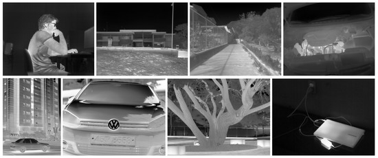
Figure 6.
Examples of test dataset (top: from []; bottom: from []).
During training, the training images were converted to the brightness domain, and the patch size of the image was set to 48 by 48 with a stride of 24 for overlap. In addition, the training data were augmented based on rotating by 90, 180, and 270 degrees, as well as flipping vertically. A total of 55,040 patches were used for training. The code was implemented in Pytorch with a 1080Ti GPU, and the learning rate was initialized to 13 until 50 epochs.
The input images for the test were generated by downsampling the ground truth and then upsampling to the original size using bicubic interpolation with scale factors ×2, ×3, and ×4.
4.2. Ablation Studies
We conducted ablation studies to validate the role of each component in our proposed approach, including the combination module, confidence-based residual, and mixed feature module. Furthermore, the optimal level of the sub-network was determined to achieve the highest performance. Figure 7 shows each network architecture in which the skip-connection is not drawn for simplification. The PSNR was adopted for the performance evaluation metric.
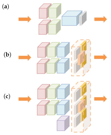
Figure 7.
The networks (a) without and (b) with the combination module. (c) The network has both the combination module and the mixed feature module.
First, the two-level networks were compared to verify the effect of the combination module with both a residual image and a confidence map. The network depicted in Figure 7a simply concatenates the output feature maps of the mapping module and then estimates the residual image through the reconstruction module. Since the confidence map was not used in this case, the output of the reconstruction module was one-dimensional. The reconstruction module in the network depicted in Figure 7b rather yielded two dimensions, a residual image and a confidence map, which were utilized in the combination module. In other words, the reconstruction module in this architecture received the output feature maps of the mapping module and generated a residual image and a confidence map. The confidence maps were used to generate the final result through the combination module.
It can be observed that the quality of an output depends on whether the combination module is applied or not, as shown in the first and second rows in Table 3. The network trained with the combination module better enhances a thermal image.
Table 3.
Performance comparison w.r.t. the combination module and the mixed feature module (blue-colored: the best case).
We now study the performance of the networks trained with the mixed feature module. Figure 7c shows the addition of a mixed feature module to the network with the combination module depicted in Figure 7b. Each sub-network feature is mixed into one feature map in this module. The purpose of this module is to strengthen the connectivity between features of the sub-network during training.
The comparison between the last row and the second row in Table 3 intuitively conveys that the performance was improved by adding the mixed feature module. Through the experiments, we can observe that the mixed feature and combination modules were both effective at improving the performance of thermal image enhancement.
The proposed architecture based on the network shown in Figure 7c consists of multiple sub-networks. To reflect the above experimental results, we used the mixed feature and combination modules and compared the performances obtained by different levels of sub-networks, . In addition, the network with the combination module, but without the mixed module shown in Figure 7b, was tested when the level of the sub-networks was two or three in order to further verify the effect of the mixed feature model.
As shown in Table 4, we can observe that the result of the two-level sub-networks with the mixed feature module (, , ) is better than the result of the three-level sub-networks without the mixed feature module (, , ). That is, the two-level sub-networks can even outperform the three-level sub-networks by adopting the mixed feature module. The proposed three-level network gave the best performance in the scale factor of two and three. Despite the fact that the four-level sub-networks showed the best performance at a scale of four, the three-level sub-networks turned out to be a reasonable option as our representative architecture.
Table 4.
Performance of multi-level networks (blue-colored: the best case).
In Figure 8 and Figure 9, the confidence maps and residual images are shown for each level of the sub-networks and for the mixed feature module. We can observe that the confidence maps and residual images were adaptively predicted according to different input qualities. Figure 10 shows the resulting images of the different scales obtained by our proposed network. Based on the predicted confidence maps and residual images, the details in a resulting image were improved.
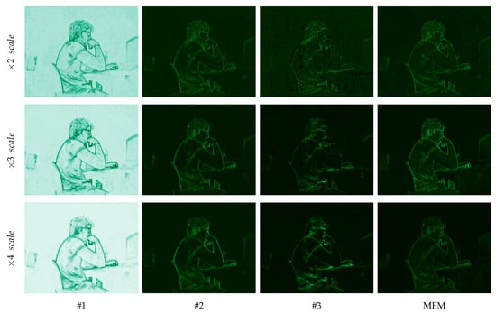
Figure 8.
Examples of confidence maps (row: scale ×2, ×3, and ×4; column: from the #1, #2, and #3 sub-networks and the mixed feature module (MFM)).
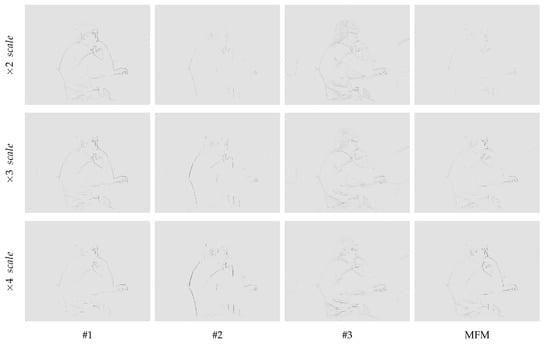
Figure 9.
Examples of residual images (row: scale ×2, ×3, and ×4; column: from the #1, #2, and #3 sub-networks and the mixed feature module (MFM)).
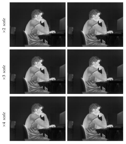
Figure 10.
Results of our proposed network (left: low-quality input image; right: enhanced output image).
4.3. Comparative Studies
We compared the representative network with the three-level sub-networks to the bicubic method and some other state-of-the-art methods: TEN [], TIECNN [], ASR2_s [], and TIR-DCSCN []. The evaluation was done on the test dataset, while the PSNR and SSIM against the ground truth were used as the evaluation metrics. In addition, line profiling [] was conducted for the in-depth analysis of the pixel values on a reference line.
Table 5 quantitatively compares the results of different methods on the test dataset. The compared methods had the limitations that each scale needed an individual network trained according to the specific scale. For example, TEN [] (×3) performed better at a scale of three than the bicubic method did, while its performance rather degraded at a scale of two as it was trained for the specific scale. TIECNN [] (×2) showed better performance in terms of both the PSNR and SSIM compared to the bicubic method at all test scales. However, note that the PSNR results of TIECNN [] (×3) and (×4) were lower than those of the bicubic method at other scales. On the other hand, it should be pointed out that our method as a single network outperformed the other compared methods at all scales. We show that a single network can be effectually trained to deal with different scale conditions.
Table 5.
The average results of the PSNR and SSIM for scale factors ×2, ×3, and ×4 (-: when it is impossible to measure due to the network structure; blue-colored: the best case).
Figure 11, Figure 12 and Figure 13 qualitatively compares the results of different methods with a scale factor of four. Two specific regions in an image are enlarged to effectively show and emphasize the enhanced details. It is worth noting that the results of our network are perceptually better, revealing more details on object boundaries. That is to say, the edges from a low-quality input image are effectively reconstructed to be of higher quality. Moreover, the texture around an edge is well preserved while enhancing the low-quality thermal image. When observing the red colored and blue-colored boxes in Figure 11, the result of our proposed method looks clear and resembles the ground truth, while the other methods are relatively blurry. As presented in Figure 12, our proposed method better minimizes the deformation of a regional detail (e.g., the black regions in the red-colored box) and produces clear edges (e.g., the horizontal boundary in the blue-colored box). Our method also fairly preserves the texture information, i.e., temperature value, at and around the pixels where the details are restored. Compared to the noisy or blurry edges obtained by the compared methods, our method recovers as much detail as the ground truth image has (see Figure 13).
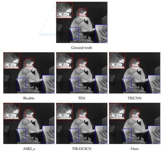
Figure 11.
Qualitative comparison on the test dataset ([]-thermal_089-S).
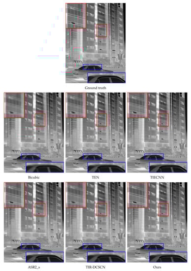
Figure 12.
Qualitative comparison on the test dataset ([]-T138-No.28).
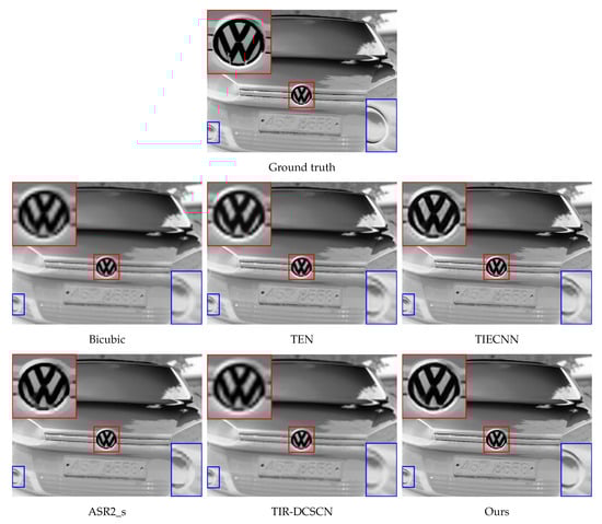
Figure 13.
Qualitative comparison on the test dataset ([]-T138-No.1).
Lastly, to analyze the pixel values of the enhanced thermal images, we performed line profiling [] on the test images with a scale factor of four. This metric was used to directly analyze and compare the thermal information to the ground truth. To evaluate a line profile in our experiment, firstly, horizontal or vertical lines were set, as shown in Figure 14 (green-colored line in the left column). Then, the absolute difference between the pixel values of the ground truth and those of the enhanced image on the line was calculated. Finally, the mean and standard deviation were computed using the values of the absolute difference. As shown in Figure 14 (right column), it can be observed that our method is more similar to the ground truth than other methods. In particular, within the positions on the line from 160 to 170 on Line 3 in Figure 14, it can be seen that the curves of the other methods have a smoother slope compared to the ground truth, whereas our method shows the most similar curve to the ground truth. Table 6 presents the comparison of the mean and standard deviation of the absolute value difference between the ground truth and each method on Lines 1, 2, and 3 in Figure 14, respectively. The smaller the mean and standard deviation are, the more similar the result is to the ground truth. Our proposed method outperforms the compared methods in line profiling, as shown in Table 6.
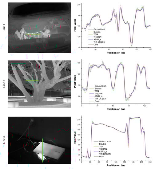
Figure 14.
Comparison of line profiles (green-colored line) for the quantitative analysis using pixel values (top: []-thermal_072-S, middle; []-T138-No.48; bottom: []-T138-No.30).
Table 6.
Evaluation of the mean and standard deviation of the difference between the ground truth and enhanced results in the line profiles (blue-colored: the best case).
5. Conclusions
The objective of this study was to enhance the low quality of a thermal image regardless of scale variation based on a single network. To achieve this objective, we introduced a novel parallel architecture leveraging the confidence maps of multiple levels. Our approach includes the mixed feature module that enhances connectivity among sub-networks and the combination module that is incorporated with the residual and confidence values. Through ablation studies, it was shown that each module was effective in enhancing the quality of a thermal image. Our method not only outperformed the comparing methods in the quantitative evaluation, but also produced perceptually better results when visually compared. In this study, we show that the networks for an individual scale can be integrated by our proposed architecture as a single network.
Author Contributions
Y.B. and K.L. conceived of and designed the experiments; Y.B. and K.L. analyzed the data; Y.B. and K.L. wrote the paper; Y.B. performed the experiments. All authors read and agreed to the published version of the manuscript.
Funding
This work was supported by the National Research Foundation of Korea (NRF) grant funded by the Korea government (MSIT) (No. 2020R1G1A1102041).
Conflicts of Interest
The authors declare no conflict of interest.
Abbreviations
The following abbreviations are used in this manuscript:
| PSNR | Peak signal-to-noise ratio |
| SSIM | Structural similarity |
| MFM | Mixed feature module |
References
- Kwaśniewska, A.; Rumiński, J.; Rad, P. Deep features class activation map for thermal face detection and tracking. In Proceedings of the 2017 10th international conference on human system interactions (HSI), Ulsan, Korea, 17–19 July 2017; pp. 41–47. [Google Scholar]
- Fernandes, S.L.; Rajinikanth, V.; Kadry, S. A hybrid framework to evaluate breast abnormality using infrared thermal images. IEEE Consum. Electron. Mag. 2019, 8, 31–36. [Google Scholar] [CrossRef]
- Tong, K.; Wang, Z.; Si, L.; Tan, C.; Li, P. A Novel Pipeline Leak Recognition Method of Mine Air Compressor Based on Infrared Thermal Image Using IFA and SVM. Appl. Sci. 2020, 10, 5991. [Google Scholar] [CrossRef]
- Baek, J.; Hong, S.; Kim, J.; Kim, E. Efficient Pedestrian Detection at Nighttime Using a Thermal Camera. Sensors 2017, 17, 1850. [Google Scholar] [CrossRef] [PubMed]
- Filippini, C.; Perpetuini, D.; Cardone, D.; Chiarelli, A.M.; Merla, A. Thermal infrared imaging-based affective computing and its application to facilitate human robot interaction: A review. Appl. Sci. 2020, 10, 2924. [Google Scholar] [CrossRef]
- Andoga, R.; Fozo, L.; Schrötter, M.; Češkovič, M.; Szabo, S.; Breda, R.; Schreiner, M. Intelligent thermal imaging-based diagnostics of turbojet engines. Appl. Sci. 2019, 9, 2253. [Google Scholar] [CrossRef]
- Rahman, M.A.; Hossain, M.S.; Alrajeh, N.A.; Guizani, N. B5G and explainable deep learning assisted healthcare vertical at the edge: COVID-I9 perspective. IEEE Netw. 2020, 34, 98–105. [Google Scholar] [CrossRef]
- Al-Humairi, S.N.S.; Kamal, A.A.A. Opportunities and challenges for the building monitoring systems in the age-pandemic of COVID-19: Review and prospects. Innov. Infrastruct. Solut. 2021, 6, 1–10. [Google Scholar] [CrossRef]
- Taylor, W.; Abbasi, Q.H.; Dashtipour, K.; Ansari, S.; Shah, S.A.; Khalid, A.; Imran, M.A. A Review of the State of the Art in Non-Contact Sensing for COVID-19. Sensors 2020, 20, 5665. [Google Scholar] [CrossRef]
- Choi, Y.; Kim, N.; Hwang, S.; Kweon, I.S. Thermal Image Enhancement using Convolutional Neural Network. In Proceedings of the 2016 IEEE/RSJ International Conference on Intelligent Robots and Systems (IROS), Daejeon, Korea, 9–14 October 2016; pp. 223–230. [Google Scholar]
- Lee, K.; Lee, J.; Lee, J.; Hwang, S.; Lee, S. Brightness-based convolutional neural network for thermal image enhancement. IEEE Access 2017, 5, 26867–26879. [Google Scholar] [CrossRef]
- Rivadeneira, R.E.; Suárez, P.L.; Sappa, A.D.; Vintimilla, B.X. Thermal Image Superresolution Through Deep Convolutional Neural Network. In Proceedings of the International Conference on Image Analysis and Recognition, Waterloo, ON, Canada, 27–29 August 2019; pp. 417–426. [Google Scholar]
- Gupta, H.; Mitra, K. Pyramidal Edge-maps based Guided Thermal Super-resolution. arXiv 2020, arXiv:2003.06216. [Google Scholar]
- Rivadeneira, R.E.; Sappa, A.D.; Vintimilla, B.X. Thermal Image SUPER-Resolution: A Novel Architecture and Dataset. In Proceedings of the VISIGRAPP (4: VISAPP), Valleta, Malta, 27–29 February 2020; pp. 111–119. [Google Scholar]
- Cascarano, P.; Corsini, F.; Gandolfi, S.; Piccolomini, E.L.; Mandanici, E.; Tavasci, L.; Zama, F. Super-resolution of thermal images using an automatic total variation based method. Remote Sens. 2020, 12, 1642. [Google Scholar] [CrossRef]
- Yuan, L.T.; Swee, S.K.; Ping, T.C. Infrared image enhancement using adaptive trilateral contrast enhancement. Pattern Recognit. Lett. 2015, 54, 103–108. [Google Scholar] [CrossRef]
- Zeng, Q.; Qin, H.; Yan, X.; Yang, S.; Yang, T. Single infrared image-based stripe nonuniformity correction via a two-stage filtering method. Sensors 2018, 18, 4299. [Google Scholar] [CrossRef]
- Lee, J.; Ro, Y.M. Dual-Branch Structured De-Striping Convolution Network Using Parametric Noise Model. IEEE Access 2020, 8, 155519–155528. [Google Scholar] [CrossRef]
- Liu, Y.; Wang, Z.; Si, L.; Zhang, L.; Tan, C.; Xu, J. A non-reference image denoising method for infrared thermal image based on enhanced dual-tree complex wavelet optimized by fruit fly algorithm and bilateral filter. Appl. Sci. 2017, 7, 1190. [Google Scholar] [CrossRef]
- Ibrahim, H.; Kong, N.S.P. Brightness preserving dynamic histogram equalization for image contrast enhancement. IEEE Trans. Consum. Electron. 2007, 53, 1752–1758. [Google Scholar] [CrossRef]
- Bai, X.; Zhou, F.; Xue, B. Infrared image enhancement through contrast enhancement by using multiscale new top-hat transform. Infrared Phys. Technol. 2011, 54, 61–69. [Google Scholar] [CrossRef]
- Van Tran, T.; Yang, B.S.; Gu, F.; Ball, A. Thermal image enhancement using bi-dimensional empirical mode decomposition in combination with relevance vector machine for rotating machinery fault diagnosis. Mech. Syst. Signal Process. 2013, 38, 601–614. [Google Scholar] [CrossRef]
- Kuang, X.; Sui, X.; Liu, Y.; Chen, Q.; Gu, G. Single infrared image enhancement using a deep convolutional neural network. Neurocomputing 2019, 332, 119–128. [Google Scholar] [CrossRef]
- Berg, A.; Ahlberg, J.; Felsberg, M. A thermal object tracking benchmark. In Proceedings of the 2015 12th IEEE International Conference on Advanced Video and Signal Based Surveillance (AVSS), Karlsruhe, Germany, 25–28 August 2015; pp. 1–6. [Google Scholar]
- Palmero, C.; Clapés, A.; Bahnsen, C.; Møgelmose, A.; Moeslund, T.B.; Escalera, S. Multi-modal RGB–Depth–Thermal Human Body Segmentation. Int. J. Comput. Vis. 2016, 118, 217–239. [Google Scholar] [CrossRef]
- Portmann, J.; Lynen, S.; Chli, M.; Siegwart, R. People detection and tracking from aerial thermal views. In Proceedings of the 2014 IEEE International Conference on Robotics and Automation (ICRA), Hong Kong, China, 31 May–7 June 2014; pp. 1794–1800. [Google Scholar]
- Morris, N.J.; Avidan, S.; Matusik, W.; Pfister, H. Statistics of infrared images. In Proceedings of the Computer Vision and Pattern Recognition, CVPR’07, Minneapolis, MN, USA, 17–22 June 2007; pp. 1–7. [Google Scholar]
- Hwang, S.; Park, J.; Kim, N.; Choi, Y.; So Kweon, I. Multispectral pedestrian detection: Benchmark dataset and baseline. In Proceedings of the IEEE Conference on Computer Vision and Pattern Recognition, Boston, MA, USA, 7–12 June 2015; pp. 1037–1045. [Google Scholar]
- Choi, Y.; Kim, N.; Hwang, S.; Park, K.; Yoon, J.S.; An, K.; Kweon, I.S. KAIST multi-spectral day/night data set for autonomous and assisted driving. IEEE Trans. Intell. Transp. Syst. 2018, 19, 934–948. [Google Scholar] [CrossRef]
- Wang, Z.; Bovik, A.C.; Sheikh, H.R.; Simoncelli, E.P. Image quality assessment: From error visibility to structural similarity. IEEE Trans. Image Process. 2004, 13, 600–612. [Google Scholar] [CrossRef] [PubMed]
- Yamanaka, J.; Kuwashima, S.; Kurita, T. Fast and accurate image super resolution by deep CNN with skip connection and network in network. In Proceedings of the International Conference on Neural Information Processing, Guangzhou, China, 14–18 November 2017; pp. 217–225. [Google Scholar]
- Zhu, J.Y.; Park, T.; Isola, P.; Efros, A.A. Unpaired image-to-image translation using cycle-consistent adversarial networks. In Proceedings of the IEEE International Conference on Computer Vision, Venice, Italy, 22–29 October 2017; pp. 2223–2232. [Google Scholar]
- He, K.; Zhang, X.; Ren, S.; Sun, J. Delving deep into rectifiers: Surpassing human-level performance on imagenet classification. In Proceedings of the IEEE International Conference on Computer Vision, Santiago, Chile, 13–16 December 2015; pp. 1026–1034. [Google Scholar]
- Kingma, D.P.; Ba, J. Adam: A method for stochastic optimization. arXiv 2014, arXiv:1412.6980. [Google Scholar]
- Yang, J.; Wright, J.; Huang, T.S.; Ma, Y. Image super-resolution via sparse representation. IEEE Trans. Image Process. 2010, 19, 2861–2873. [Google Scholar]
Publisher’s Note: MDPI stays neutral with regard to jurisdictional claims in published maps and institutional affiliations. |
© 2021 by the authors. Licensee MDPI, Basel, Switzerland. This article is an open access article distributed under the terms and conditions of the Creative Commons Attribution (CC BY) license (http://creativecommons.org/licenses/by/4.0/).