1. Introduction
Dynamical processes in the neuron [
1] include, among others, those concerning the release of neurotransmitter (NT) into the synaptic cleft. The release occurs via calcium channels [
2,
3] and the amount of the released NT is measured indirectly by the postsynaptic potential. In
Figure 1A in the cited paper [
3] the connection between NT amount and postsynaptic current is illustrated; in Figure 3C in other work [
4] the shape of the impulse in genetically different animals is presented; diminished amplitude means impaired genotype. The above mentioned dynamical processes are often described by using differential equations [
5,
6,
7], including—for a long time—partial ones [
8,
9,
10]. The equation of this type can not, usually, be solved analytically, and therefore numerical methods have to be used [
10,
11,
12,
13]. In order to perform the calculations quickly and accurately, the appropriately designed mesh, in the nodes of which the calculations will be made, should be created. In biological sciences the boundary conditions are generated by the modeled organelles in biological structure of the cell. For example, what the model should take into account is the work of the active zone of the presynaptic bouton during exocytosis. It is one of the crucial mechanisms in transmitting nerve impulses and it is accomplished by means of
channel (one of three kinds of similar channels:
,
and
) [
4]. Therefore, the design of a good mesh is a difficult problem connected with the mesh geometrical properties [
14,
15]. Tetrahedral meshes are also studied in the context of automatic adjustment [
16]. Finite Elements Method, on the other hand, requires a high quality mesh [
17]. This means that a single cell should be as regular as possible—an equilateral triangle in two dimensions, and in the 3D case—a regular tetrahedron. Generally, it is impossible to reach this goal in practice because of the geometric properties of the modeled object. Additionally, regular tetrahedra can not be used as elements of a spatial mesh. In reality, such tetrahedra differ in shape and size; also, the regions joining different parts of the model are usually covered with elements of worse quality.
In this paper the problem of dependence of numerics precision on the quality of the spatial data structure (a tetrahedral mesh) for numerical calculations for processes in the neuron axon terminal is studied. Various geometrical presynaptic bouton models are discussed. They are compared by using several different parameters of the quality of the mesh, one of them formerly introduced [
18]. The differences in the results of simulations for different meshes, with other parameters kept unchanged, are analyzed. The adequate measure of the differences is the amount of neurotransmitter released to the synaptic cleft.
This paper is a continuation of the studies described in [
6,
8,
11,
12,
18,
19,
20,
21,
22].
2. Model
Since the transport of neurotransmitter (NT) in the presynaptic bouton of the neuron has to be considered both in spatial and in temporal aspect, the partial differential equation model has been introduced, derived from the diffusion equation with nonlinear modifications. The more detailed description of the model is presented in [
8]. Main aspects of the model are given below.
2.1. Diffusive PDE Model
When setting up the model, the following was assumed:
The presynaptic bouton occupies a bounded subset
of three-dimensional space. The NT supply takes places in the bouton subdomain
(supply zone), thereby increasing the total amount of NT in the bouton. On the other hand, the release through the subset
of the bouton membrane
decreases that amount. The NT flow in the presynaptic bouton, basing on the similar study [
22], was modeled with the following partial differential Equation (
1):
where
is the density of NT at time
t and at the spatial location
x and
a is the diffusion coefficient. The appropriate initial conditions had to be set and, similarly, the boundary conditions [
22] should be modeled by the Equation (
2)
where
is the permeability coefficient and
is a directional derivative in the outer normal direction
. The function
(depending on time
t) takes the value of 1 for
(with the action potential arriving at
and with the release time
), and
otherwise [
19]. In such a way, boundary conditions are a simple model of exocytosis through a
type voltage-gated channel.
When the Equation (
1) is multiplied by a smooth function
, and after integrating by parts [
22], we obtain
which is valid when
is sufficiently smooth.
2.2. 3D Simulations—The Finite Elements Method
Piecewise linear
finite elements (tetrahedra) are used to perform the calculations according to the numerical scheme [
22]. The function
, which approximates
, is calculated as
where
are the basis functions of the finite elements space. When the following matrices are introduced: The mass matrix
, the stiffness matrix
, and the release matrix
, and when the additional assumption is made that
, and the nonlinear operator
is applied according to [
22]:
the numerical scheme may be rewritten as
The time step is defined as
where
is at least several times smaller than
. After the approximation of
by
, the Crank–Nicholson approximative scheme can be used
valid for
. In the finite element basis
,
is approximated by
. The scheme must be solved for
. The problem of the nonlinearity in
is dealt with by the iterative scheme:
in which the inner iteration step is denoted by the index
m. In such a way, the scheme gives a linear system of equations for each iteration. Iterating stops when
is sufficiently small.
For the numerical simulations, the bouton is modeled as a bounded polyhedral domain . The boundary of the bouton, , is represented by a set of flat polygons. The proper polyhedral subset of the bouton, , is the domain of vesicles supply. The release site is modeled as a finite sum of flat polygons.
3. Generation of the Mesh
As it has already been mentioned [
18], the problem of generating a mesh of a complex object is difficult. Firstly, a reasonable compromise must be found between a mesh with a very large number of small tetrahedra (increased computing time) and another one with a small number of relatively large elements (errors in simulating flow near tiny substructures). Secondly, the mesh elements should be as regular as possible [
23].
3.1. Mesh Element Quality
The mesh quality parameters, considered below and calculated for each element, are as follows.
Assuming that
S denotes the total surface, and
—the total volume of the tetrahedron, the following parameters have been used [
18]: The first of the defined parameters was
The second parameter was the ratio of the longest edge and the radius of the inscribed sphere [
24]:
ranging from
, for a regular tetrahedron, to infinity.
The third one is the value applied in the TetGen program [
25,
26] i.e., the longest edge divided by the smallest height (EH)
with the range similar as in the previous example i.e., from
to infinity, following the same rule as before: “the larger the value, the worse the tetrahedron”.
The last two parameters are and , and they are computed as the ratios of the largest () or the smallest () face measure, respectively, to the total surface (S) of the tetrahedron.
The formula for the first of those two parameters is
and its value ranges from 0.25 to 0.5 i.e.,
The formula for the second parameter is
and its value ranges from 0 to 0.25 i.e.,
The parameters mentioned above (SV, ER, EH, MAXS and MINS) is positive and dimensionless. All of them, except MINS, have the smallest value for the regular tetrahedron. The MINS value behaves differently: the closer to zero, the worse the tetrahedron; the maximum value 0.25 is reached for a regular tetrahedron. Moreover, the value 0.25 of both the MAXS and the MINS does not necessarily mean that the tetrahedron is regular—it may be a sliver-type (see Figure 8 in [
25]). Other irregular tetrahedron with the vertices at (−0.001,0,0), (0.001,0,0), (0,−0.001,100) and (0,0.001,100) is a wedge-type one (see Figure 8 in [
25]).
The numerical approximation of a gradient of a given function depends strongly on the largest angle (planar angle for a triangle and spherical or dihedral angle for a tetrahedron) [
27]. Thus, the condition number of the stiffness matrix should be kept to a minimum.
Theoretically, to solve a partial differential equation numerically, the above mentioned quality measures
–
should be as close to the ideal ones as possible for each of the mesh elements. However, not all deviations from the ideal have strong negative influence on the calculations with FEM. Moreover, it turns out that tetrahedrons with faces far from optimal are still of a quality enough to be used for numerical analysis of the model [
23].
3.2. Mesh Boundary
If the structure to model is complex in a sense that it contains many substructures with their own surfaces which consist of triangles of very different size and quality then the generated mesh must take into account these substructures and the joints between them, which constitutes additional problems during the mesh generation.
The 3D mesh should be of a good quality not only in its 3D aspect but also in its 2D aspect as well. This concerns the quality of the surface of the mesh and, especially, the parts belonging to distinct areas.
The quality of a 2D (triangular) mesh of the surface of the bouton which topologically remains similar to the 3D ball is assessed analogically to the quality of the 3D net.
The quality measures that correspond to the ones defined for the spatial meshes are as follows: the square perimeter divided by the square root of the surface (PS2), the longest edge divided by the radius of the inscribed sphere (in that case the 2D sphere is a circle) (ER2), the longest edge divided by the smallest height (EH2) or the function of the ratio of the largest and smallest edge length, respectively, to the total perimeter of the triangle (MAXE and MINE).
Similar as in the 3D case, the best (the smallest) attainable values of the above measures (except MINE) are:
and the largest MINE is
For the first three measures the upper bound is infinity whereas for the fourth one (MAXE) it is equal to 0.5, and the lower bound for the last parameter (MINE) is 0.
3.3. Mesh Inconsistency
One of the possible faults of the mesh results from the fact that its boundary is not a closed surface and the meshing program is trying to create elements (tetrahedra) outside the bouton (leaking) which may happen when the intended common vertices of the adjacent tetrahedra separate, creating the gap between the walls. Another example of “leaking”, termed as double edge, means that a cleft is created between the edges and the size of the cleft is less than one thousandth of the edge length. Intersection appears when the edge of one tetrahedron is intersecting with the face of another one; Some subset of the 3D mesh volume is then defined twice.
3.4. Mesh Quality
The measures of the mesh quality can by either the extreme values of the quality parameters or other parameters of the distribution of a parameter e.g., the maximum value of SV, ER, EH, or MINS, or minimum value of MAXS. These quantities, that are sometimes used to describe the mesh, and also the distributions themselves, are presented as tables and histograms.
4. Geometrical Models of the Bouton
The geometry of the bouton was modeled in three various ways, using three different objects.
Two of them—the geosphere and the ball (globe)—were extremely simplified models. The basic difference between geosphere surface mesh and globe surface mesh is that the geosphere surface consists only of triangles, nearly equally-shaped and nearly equilateral, whereas the globe surface contains two types of polygons: (1) equal isosceles (but not necessarily equilateral) triangles; and (2) trapezoids. The two above models are known to differ in some aspects. Two of them are most commonly mentioned. The first one is that with the globe mesh it is easier to create shapes with edges along meridians and circles of latitude. The second one is that with the geosphere mesh it is easier to make a relatively smooth surface with a smaller number of mesh elements.
The third model, so-called real model, reflected the real geometry of the bouton surface and accounted for the presence of the inner organelles—see [
20] for details.
4.1. Geosphere—The Simplest Model of the Sphere
The two-dimensional geosphere surface mesh, often used, for example in [
18], to depict the surface of a sphere, consists of triangles, which are almost equilateral. Their characteristics exceed the ideal values by 1.3% to 25.5% which constitutes a good reference point for comparison of the quality of 3D meshes. The analyzed surface (
Figure 1, left) had 15,680 triangular faces and 7482 vertices.
The quality of the model of the geosphere surface is presented in
Table 1.
The angles of the triangular mesh considered in
Table 1 vary between the values of
and
. The range of triangle area was from
to
. Therefore, the ratio
was
. The surface mesh was then submitted as the input data to the TetGen program which produced the tetrahedral mesh of the sphere (
Figure 1, right).
The parameters of the sphere were as in
Table 2.
These parameters are the reference point for the next calculations.
4.2. The Ball (Globe)—The Simplest Geometric Model of the Presynaptic Bouton
The globe is a sphere divided into spherical polygons by meridians and circles of latitude. A typical globe is a depiction of the Earth’s surface. For example, one may draw a globe with 24 meridians and 13 circles of altitude—or rather 11, if we exclude poles as degenerate circles. The simplest object used for modeling a presynaptic bouton [
19] consisted of two such globes placed concentrically (see
Figure 2).
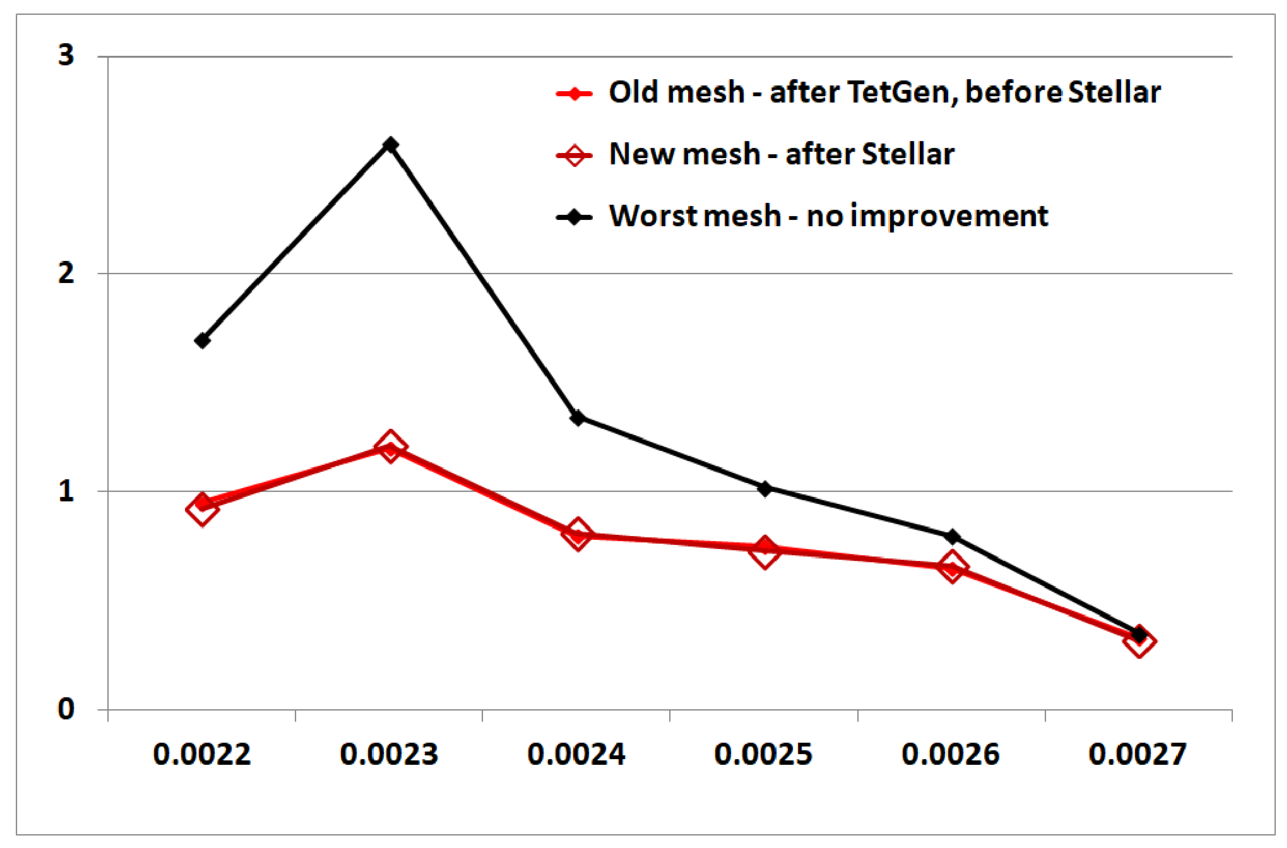
The input parameters for the meshing software were as follows: maximum volume of a single mesh element (tetrahedron) (). Another two important parameters are the maximum aspect ratio () which is not standardized but computed directly as the ratio of the longest edge and the shortest height of a tetrahedron. The last restriction is that of the minimum dihedral angle (). It should be stressed that the last restriction is the most strictly observed in the program.
The 2-dimensional mesh is generated in such a way that each spherical polygon is replaced by a flat polygon with vertices at the same points. The quality of the globe mesh was tested in the following subspace of the above parameters:
The example results of these tests are presented in
Figure 3:
for the fixed values of and and for ranging from to ;
for the fixed values of and and for ranging from 0.0006 to 0.0015.
The best quality was achieved when the imposed restrictions were: , and .
The input 2D mesh and the results of its tetrahedralization are presented in
Table 3 and
Table 4.
4.3. The Real Model with Inner Organelles
In the real model, the shape of the bouton surface is created on the basis of the microscope image [
28]—see [
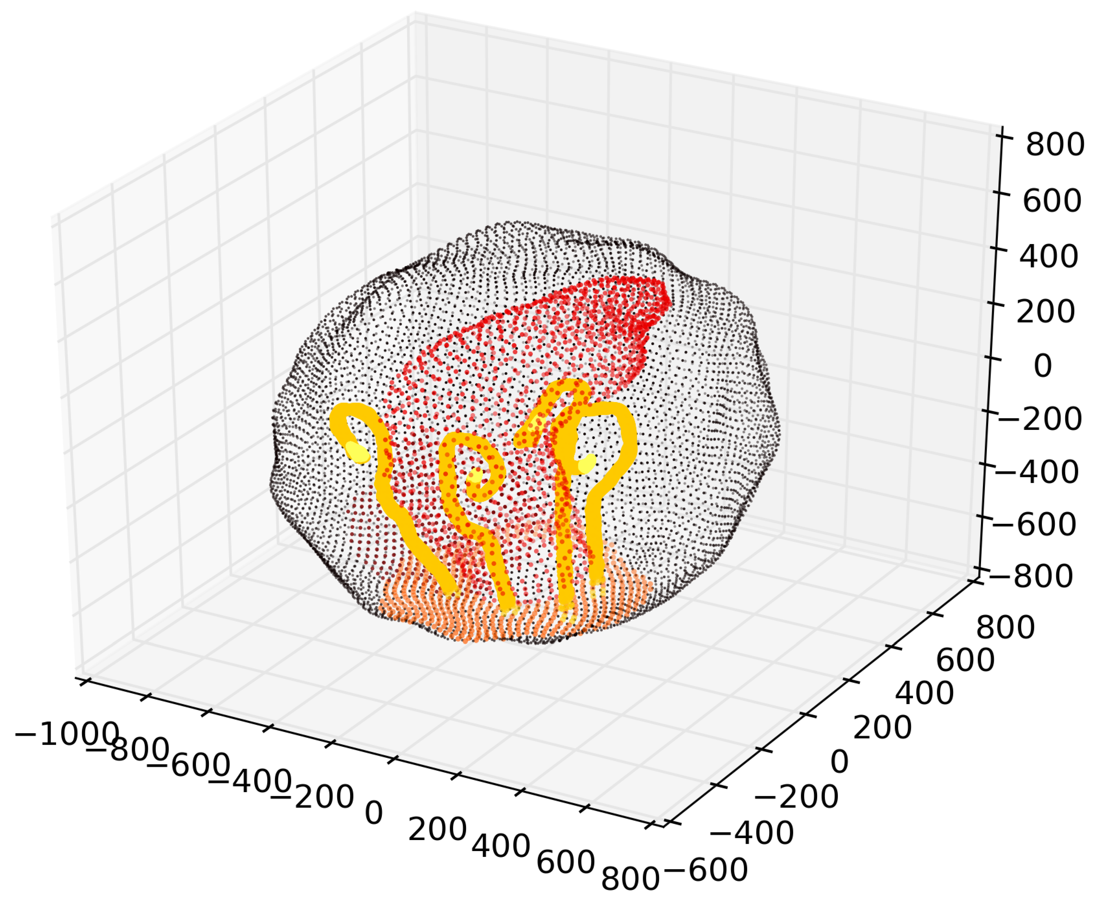
20] for details concerning the way the model is generated. Furthermore, the inner organelles—mitochondrion and microtubules—are also modeled as the inner structures of the bouton—
Figure 4. In the model the following areas have to be taken into consideration: the area of the synapse membrane in general, the zone of releasing the neurotransmitter particles, the surface of the mitochondrion which in our model is connected to the artificially (i.e., numerically) cut bouton, the surface of the microtubules and of microtubule terminals. The above surfaces are marked with different colors in the graphs—
Figure 5.
The input mesh was made up of 41,807 vertices and 83610 triangles—
Figure 6. Generation of the three-dimensional mesh in such a way that the triangular faces of the mesh tetrahedra constitute the two-dimensional mesh covering the surfaces of the inner structures, especially when small details are concerned, was one of the crucial problems (
Figure 5,
Figure 6,
Figure 7,
Figure 8 and
Figure 9, in particular
Figure 5 and
Figure 9, see also [
17]). The characteristics of the input mesh are presented in
Table 5.
The above input mesh was passed as input data to the TetGen program. The program generated output mesh with no optimization, thereby the result was deliberately of a very poor quality. The parameters of the output tetrahedral mesh are presented in
Table 6. The mesh had 57,060 nodes, 114,116 boundary faces and 194,064 tetrahedra.
The next step was, as it has been done previously, to generate the optimized mesh. Its quality was checked for different values of input TetGen parameters. Those parameters after preliminary tests were set to
= 1000
The best quality was achieved for .
The size of the mesh was 391,897 nodes, 4,141,116 faces (296,528 on the bouton surface) and 1,996,426 tetrahedra.
5. First Comparison of the Models
The quality of all 3D meshes of the models are given in
Table 8. The smallest values are always close to the ideal ones; the relative differences was always below 1.23% so those minimal numbers are not presented.
For the simplified models of the bouton (the geosphere and the globe)
Table 8 the distance between the mean and the median lay within the range of two standard deviations of the corresponding parameter.
For the real model of the bouton, that takes into consideration the same parameters, the situation was noticeably worse, although it still remained satisfactory. The specified 90th and 99th percentiles were similar for all three models. The maximal values in the case of the real bouton mesh were, however, over one order of magnitude (approximately 30 times) larger than the corresponding values for the simpler models which means that there are some bad quality mesh elements. Nevertheless, their number is extremely low in comparison to the total number of the mesh tetrahedra.
If the simplest structures are to be taken as the reference points for assessing the quality of the real mesh, it must be admitted that the extreme values of the quality parameters (non-standardized) were significantly higher than those reference values. The percentage of the “bad” tetrahedra was, however, low—below 1%, which means that, in general, the meshes were suitable as the input for subsequent optimizations.
6. Further Optimizations Involving Modifications of the Surface and Improvement of Dihedral Angles
The results of examination of the created meshes, particularly the real one, revealed problems with their quality, mainly concerning the distribution of dihedral angles of mesh elements, so additional modifications were needed. That was accomplished by using the Stellar software [
29]. Next, the simulation results for the worst mesh were compared with those for the best one.
The Stellar program performs transformations like inserting and deleting vertices, edge contraction, smoothing or removing boundary or near-boundary nodes, removal of boundary edges, multi-face removal and, in addition, compound operations which means combinations of all the above transformations.
Stellar software focuses mainly on correcting dihedral angles of mesh tetrahedra which, according to the author, is crucial for numeric calculations (see [
29] and the relevant references therein). The results of improving that parameter are in
Table 9 for the three models presented above.
The extreme values of the parameters SV, ER, EH, MAXS and MINS after improving the mesh are given in
Table 10.
7. Simulations
As it has been mentioned above, the last method applied in this paper to compare the quality of meshes was to run example simulations for the different meshes of the same object and comparing the results. The three 3d “real” meshes were chosen: the mesh with no improvement, the one improved by TetGen and the mesh which was additionally optimized with Stellar. The parameters for all three simulations were the same: the size and shape of the surface mesh, the initial density distribution of neurotransmitter (NT), the time step assumed for the calculations and the time interval during which the release of NT took place.
The values determining the results used in this paper were: diffusion coefficient /s, permeability coefficient /s, the time step s and the time interval during which the release occurred—from s to s.
The criterion used to compare the results was the amount of neurotransmitter released during the first release time interval i.e., from s to s, which embraced 6 consecutive time steps. The additional criterion connected with the first one was the total amount of NT in the bouton.
8. Results
The results are presented in
Figure 13. Three plots break down naturally in two groups. The two lower ones, depicting the total amount of neurotransmitter (NT) in the bouton varying in time, are almost identical. The values for the mesh improved with Stellar are only a little lower. This may be attributed to the fact that the total amount of NT was calculated based from the values of the density function in mesh vertices which differed in number and location between meshes. The upper plot (black) refers to the initial unimproved mesh. Its values are remarkably higher and the differences are clearly visible; nearly doubled values at the beginning of the impulse and equal values at the end.
Two out of five values of the real mesh parameters presented in
Table 8 increased remarkably after applying Stellar optimization. Namely, the maximal value of ER changed from 605.7 to 838.5 and the maximum of EH—from 301.5 to 383.6. The corresponding 95th percentiles decreased which means that only a very small fraction of the tetrahedra had worse ER or EH quality. The maximal (in case of MINS, minimal) values and the 95th (for MINS, the 5th) percentiles of of all other parameters improved after optimization. The interesting outcome of the optimization is that the only parameter that showed substantial improvement was the one designed for this paper i.e., the SV parameter which changed from 8.83 to 6.40 (a nearly 30% better value). The results confirm that the parameter SV could be calculated instead of six dihedral angles of a tetrahedron. With the improved mesh, simulation of neurotransmitter flow in the examined model should be performed with sufficient precision. The detailed inspection of the accuracy of these calculations will be the subject of further research.
It should be stressed that the mesh analyzed in this paper is quite a complicated one which can be confirmed by the fact that the output mesh quality measured by dihedral angles was only in the range of 19 to 160 degrees. When we take into consideration the statement from [
29]: “
My implementation usually improves meshes so that no dihedral angle is smaller than or larger than ”, it must be concluded that the mesh considered here is extremely complicated.
9. Effect of Mesh Quality on the Algorithm Performance and Results of Simulations
The algorithm, basically, consists of two modules. The first one is responsible for calculations initialization. Among others, it initializes the vector of the unknown variables i.e., the density vector . The second one performs iterative calculations over time and space mesh.
In the second module, the iterative one, the calculations in each iteration are divided into three steps: the first one, during which the equation system is solved without taking release and synthesis into consideration, the second one when the values of the vector are updated with the synthesis, and the third one, that involves the diminishing the value of the neurotransmitter density by the amount resulting from the exocytosis. Within the second said step, solving the equation system must be repeated until the status of each tetrahedron—“producing” or “non-producing”—is established between iterations. This means, among others, that calculations on a single tetrahedron may cause the program get stuck in the loop in case when the tetrahedron has one vertex in the release zone and another one in the synthesis zone. Such vertices exist in the worst, unimproved mesh in the real model.
In general, the comparison of calculations for different meshes is a difficult task. The reason is that vertices of different meshes covering the same object, are usually not identical. Therefore it is not possible to compare results obtained in the same mesh points. In the case of modeling the dynamics of transmitting signals in synapse, however, the situation is convenient because the total release of neurotransmitter into synaptic cleft in the time unit is a direct effect of the run of the processes occurring in the presynaptic bouton. This directness is guaranteed by the fact that the presynaptic bouton, considered as a cybernetic system, has the observability property [
6].
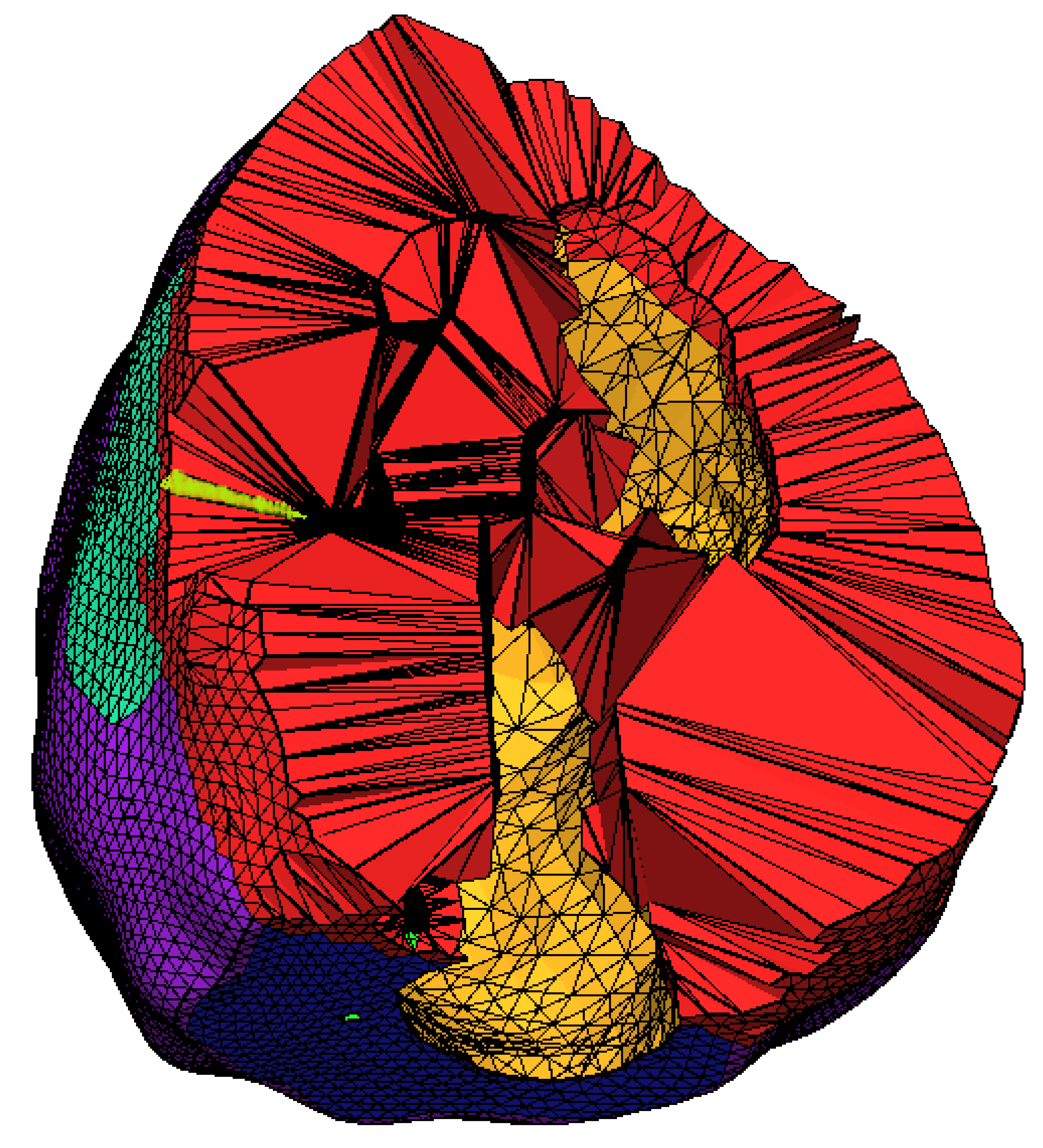
Referring to the conducted simulations, the phenomena mentioned above are visible clearly. First of all, for the worst unimproved mesh, the calculations with the synthesis turned on got stuck in a loop because of existence of tetrahedra that intersect both the release area and the synthesis area. Such an example tetrahedron is marked bright lime in
Figure 7.
In the case of simulation without synthesis, the total amount of neurotransmitter released into the synaptic cleft differs by a factor of around two, for the worst mesh (Mesh 1) compared to the middle-quality one (Mesh 2) and the best mesh (Mesh 3) which both give practically the same result—see
Figure 13 and
Table 11. The remarkable difference in the simulated amount of released neurotransmitter means, among others, that even in the case of a simple dynamic model—diffusive-reactive PDE model—the use of a mesh of a poor quality produces results which do not reflect the real solutions. It must be admitted that the shape of the impulse is maintained, and that can be confirmed by comparing impulses conducted via calcium channels measured by other authors [
2,
3] with the result of our research. In all the papers, including this one, the impulses were V-shaped. It should be also noted that the amount of the released NT, used in this paper, is a very accurate indirect measure of the postsynaptic potential (see Figure 1A in the related work [
3]). The peak of the impulse, however, is higher for the worst mesh (
Figure 13) which would lead to false conclusions. In genetic research this could even favor the object which produces higher output amplitude as more heterozygous since homozygosity usually means impairing life processes (see a related paper [
4], especially
Figure 3C therein).
The performed simulations, furthermore, shed—to some extent—light on the problem of the mesh quality in the context of dynamical numerics applications. Namely, in the assessment of the mesh quality the common view is that the dihedral angle between the tetrahedron faces is a significant parameter determining the mesh quality—for the ideal mesh the measure of the dihedral angle between any faces should be
. Therefore, the Stellar package is oriented mainly towards improving that parameter The simulations presented in this paper indicate, however, that at least for the diffusive-reactive model the improvement of the parameter connected with the quality of dihedral is not of a great importance—compare the results for Mesh 2 and Mesh 3 in
Table 11. Apart from the fact that after applying Stellar package the dihedral angle parameter of the Mesh 3 is significantly better than that of Mesh 2—
Table 9—the results for the both meshes are practically the same.
10. Concluding Remarks
As it has been aforementioned in Introduction, the main objective of this paper was to discuss the specifics of the quality measures of the generated mesh with respect to numerical calculations and fidelity of simulations. The obtained results lead to the following conclusions.
In the situation similar to that considered in this paper, the low quality mesh may alter the results of numerical simulations by a factor greater than two. In the context of modeling transmission of signals in the synapse such a low-fidelity result makes the simulation useless.
In the contrary to opinions expressed in a few papers, the dihedral angle in the case of our simulations did not prove an important parameter determining the quality of the simulation in the considered case.
The problem of generating the three-dimensional mesh itself is not trivial [
30,
31]. If the geometry of the simulated object is relatively simple—in our example, a geosphere or a globe with regular internal structures (like the spherically-shaped domain of neurotransmitter supply)—then generation of a 3D mesh of the object does not cause radical problems. The tetrahedral mesh generator like TetGen can easily produce a mesh of a satisfying quality (
Table 2,
Table 4, and
Figure 1). On the other hand, if the geometry of the model is complex, then generation of the mesh is faced with essential difficulties. Even such dedicated software as TetGen is not always capable of dealing with the problem. The quality of the created mesh is significantly worse (see
Table 7 as well as
Figure 10,
Figure 11 and
Figure 12). However, even moderately optimized meshes seem to produce satisfying results.


