Various Generative Adversarial Networks Model for Synthetic Prohibitory Sign Image Generation

Abstract

A synthetic image is a critical issue for computer vision. Traffic sign images synthesized from standard models are commonly used to build computer recognition algorithms for acquiring more knowledge on various and low-cost research issues. Convolutional Neural Network (CNN) achieves excellent detection and recognition of traffic signs with sufficient annotated training data. The consistency of the entire vision system is dependent on neural networks. However, locating traffic sign datasets from most countries in the world is complicated. This work uses various generative adversarial networks (GAN) models to construct intricate images, such as Least Squares Generative Adversarial Networks (LSGAN), Deep Convolutional Generative Adversarial Networks (DCGAN), and Wasserstein Generative Adversarial Networks (WGAN). This paper also discusses, in particular, the quality of the images produced by various GANs with different parameters. For processing, we use a picture with a specific number and scale. The Structural Similarity Index (SSIM) and Mean Squared Error (MSE) will be used to measure image consistency. Between the generated image and the corresponding real image, the SSIM values will be compared. As a result, the images display a strong similarity to the real image when using more training images. LSGAN outperformed other GAN models in the experiment with maximum SSIM values achieved using 200 images as inputs, 2000 epochs, and size 32 × 32.

1. Introduction

Neural networks with more layers have been implemented in the latest development in deep learning [1]. These neural network models are far more capable of acquiring greater preparation. Nonetheless, obtaining a correct and reliable data collection with manual labeling is often costly. In machine learning as well as computer vision, this has been a general problem. An effective way to synthesize images is to increase the training collection which will improve image recognition accuracy. Employing data augmentation for enlarging the training set in image classification has been carried out in various research [2]. Traffic sign detection (TSD) and traffic sign recognition (TSR) technology have been thoroughly researched and discussed by researchers in recent years [3,4]. Many TSD and TSR systems consist of large quantities of training data. In recent years, a few datasets of traffic signs have been shown: German Traffic Sign Data Set (GTSRB) [5], Chinese Traffic Sign Database (TSRD), and Tsinghua-Tencent 100K (TT100K) [6]. Traffic signs are different from country to country and, in various circumstances, an interesting recommendation is to apply synthetically generated training data. The synthetic image will save time and energy for data collection [7,8]. Synthetic training data have not yet been commonly used in the TSR sector but are worth exploring because very few datasets come from other countries, in particular from Taiwan. In this research, we focus on Taiwan’s prohibitory signs. Our motivation arises from the current unavailability of such a Taiwan traffic sign database, image and research system.

A generative adversarial network (GAN) [9] is a deep research framework of two models, a generative model and a discriminative model. Both models are instructed together. GAN has brought a lot of benefits to several specific tasks, such as images synthesis [10,11,12], image-to-image translation [13,14], and image restoration [15]. Image synthesis is a fundamental problem in computer vision [16,17,18]. In order to obtain more diverse and low-cost training data, traffic sign images synthesized from standard templates have been widely used to train classification algorithms based on machine learning [12,19]. Radford et al. [20] proposed the Deep Convolutional Generative Adversarial Network (DCGAN) in 2016. DCGAN combines the Generative Adversarial Network (GAN) with CNN so that all GANs can obtain better and more stable training results. Other versions of GAN are Least Squares Generative Adversarial Networks (LSGAN) and Wasserstein Generative Adversarial Networks (WGAN) [21,22]. Both can better solve the problem of instability training in GAN. Each GAN has achieved excellent results in producing synthetic imagery. Therefore, due to the lack of a current training dataset, our experiments apply DCGAN, LSGAN, and WGAN to generate synthetic images.

Traffic sign images compiled from regular models are commonly used to collect additional training data with low cost and flexibility to train computer classification algorithms [19]. In this paper, DCGAN, LSGAN, and WGAN are used to generate complicated images. The synthetic image is a solution for holding a small amount of data. GAN has performed outstanding results in image data generation. Our experiment favors using synthetic images by GAN to obtain image data because this does not depend on a vast number of datasets for training.

This work’s main contributions can be summarized as follows: first, a synthesis of high-quality Taiwan prohibitory sign images Class (T1-T4) is obtained using various GAN models. Second, an analysis and evaluation performance of DCGAN, LSGAN, and WGAN generates a synthetic image with different epochs (1000 and 2000), numbers, and sizes (64 × 64, and 32 × 32). Next, we proposed an experimental setting with various GAN styles to generate a synthetic image. We then evaluate the synthetic image using SSIM and MSE. The remainder of this article is structured as follows. Section 2 covers materials and methods. Section 3 describes the experiment and results. Lastly, Section 4 offers preliminary conclusions and suggests future work.

2. Materials and Methods

A synthetic picture is used to expand the dataset broadly. A well-known method is the combination of original and synthetic data for better detection performance. Multiple approaches such as [23,24] have confirmed the advantage of combining synthetic data when actual data is limited. Lately, particular approaches [25] have proposed to defeat the domain gap among real and synthetic data by applying generative adversarial networks (GANs). This system obtained more reliable results than training with real data. However, GAN is challenging to train and has shown its importance primarily in regression tasks.

2.1. Deep Convolutional Generative Adversarial Networks (DCGAN)

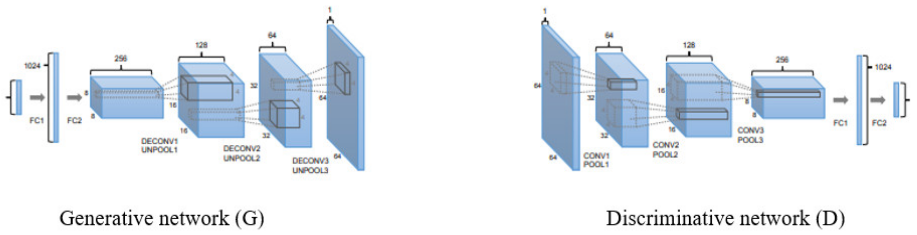
Radford et al. evaluated the architectural and topological constraints of the convolutional GAN in 2016. The method is more stable in most settings, and is named Deep Convolutional GAN (DCGAN) [20,26]. DCGAN is a paradigm for image production consisting of a generative G network and a discriminative D network [20,27]. Figure 1 displays the G and D network diagram. The G network is a neural de-convolutional device that creates images from d-dimensional vectors using de-convolutional layers. On the other hand, a D network has the same equivalent structure as a traditional CNN that discriminates whether the data is a real image from a predefined dataset or G [28]. The training of DCGAN is expressed in Formula (1) as follows [9]:

$$minimax\left(D,G\right)= {\mathbb{E}}_{x~pdata\left(x\right) }\left[logD\left(x\right)\right]+ {\mathbb{E}}_{z-p_z\left(z\right) }\left[log\left(1-D\left(G\left(z\right)\right)\right)\right]$$

(1)

where x is the first image, z is a d-dimensional vector consisting of arbitrary numbers, and $pdata\left(x\right)$ and $p_z\left(z\right)$ are the probability distributions of x and z. $D\left(x\right)$ is the probability of the input being a generated image from $pdata\left(x\right)$, and $(1-D\left(G\left(z\right)\right)$ is the probability of being generated from $p_z\left(z\right)$. D is trained to increase the correct answer rate, and G is trained to decrease $log(1-D\left(G\left(z\right)\right)$ to deceive D.

Consequently, optimizing D, we obtain maximum V (D, G), and when optimizing G, we obtain minimum V (D, G). Lastly, the optimization problem is displayed in Formula (2) and Formula (3):

$$D_G^{*}=argmaxV \left(G,D\right)$$

(2)

$$G^{*}=argminV \left(G,D_G^{*}\right)$$

(3)

G captures sample data distribution and generates a sample like real training data with noise z obedient to a certain distribution, such as uniform distribution and Gaussian distribution. The pursuit effect is as good as the actual sample. The D classification estimates the probability of a sample being taken from training instead of the from data generated. If the sample is from real training results, D gives a significant probability. Otherwise, D gives a small probability [29,30].

2.2. Least Squares Generative Adversarial Networks (LSGAN)

The discriminator in LSGANs uses the least squares as its cost function [31,32]. In other applications, LSGANs are used to generate samples that can represent the real data. There are two advantages of Least Squares Generative Adversarial Networks (LSGANs) over regular GANs. First, LSGANs can produce more extraordinary quality images than conventional GANs. Second, LSGANs perform more stably during the learning process [33,34]. Training GANs is a complex problem in practice because of the instability of GANs’ learning.

Recently, research papers have pointed out that the uncertainty of GANs’ learning is affected by the objective function [35]. In particular, decreasing the typical GAN objective functions can affect gradient loss problems, which makes it difficult to update the generator. This barrier can be relieved by LSGAN since the penalization of samples dependent on the boundary distances may create further gradients when the generator is modified. In comparison, training instability for standard GANs is focused technically on the method-searching action of the objective function, and LSGANs display fewer mode-seeking behaviors. The cost function of an LSGAN is shown in Formulas (4) and (5) [36].

$${}_{D }{}^{min}V \mathrm{LSGAN} \left(D\right)= \frac{1}{2} E \left[{\left(D\left(X_{real,i}\right)-1\right)}^2\right]+\frac{1}{2} E \left[{\left(D\left(G(X_{fake,i}\right)\right)}^2\right]$$

(4)

$${}_{G }{}^{min}V \mathrm{LSGAN} \left(G\right)= \frac{1}{2} D \left[{\left(G\left(X_{fake,i}\right)-1\right)}^2\right]$$

(5)

LSGANs can generate new data with high similarity to the original data through the mutual benefits of discriminator and generator in the model [37]. Therefore, this paper chooses LSGAN to augment the dataset and generate more realistic data.

2.3. Wasserstein Generative Adversarial Networks (WGANs)

WGAN [22] has been developed to solve the problem of network training variability [38], which is believed to be correlated with the presence of unwanted fine gradients of the GAN discriminator function. Yang et al. [39] approved WGAN for denoising low-dose CT images and attained a successful application in medical imaging reconstruction. WGAN is used in the synthesis data generation module to generate virtual damage signals to monitor the increase in minority defects and stabilize the training data set using synthetic signals.

Two important contributions of WGAN [40] are as follows: (1) WGAN may not display a sign in the experimental collapse mode. (2) When the critic performs well, the generator will always understand. To estimate the Wasserstein distance, we need to find a 1-Lipschitz function. This experiment builds a deep network to learn about the problem. Indeed, this network is very similar to the discriminator D, but without the sigmoid function, and the output is a scalar score rather than a probability. This score can be explained as how real the input images are. In WGAN the discriminator is changed to the critic to reflect its new role. The difference between GAN and general WGAN is to change discriminator to critic, along with the cost function. For both, the network design is almost the same except that the critic does not have an output sigmoid function. The cost function in critic and generator for WGAN could be seen in Formulas (6) and (7), respectively.

$${\nabla }_w\frac{1}{m}{\displaystyle \sum }_{i=1}^m\left[f\left(x^{\left(i\right)}\right)-f\left(G\left(z^{\left(i\right)}\right)\right)\right]$$

(6)

$${\nabla }_{\theta }\frac{1}{m}{\displaystyle \sum }_{i=1}^{m}f\left(G\left(z^{\left(i\right)}\right)\right)$$

(7)

However, f has to be a 1-Lipschitz function. To enforce the constraint, WGAN applies a simple clipping to reduce the highest weight value in f. The weights of the discriminator must be regulated by hyperparameters c within a certain range. The architecture of WGAN is shown in Figure 2, where z represents random noise, G represents generator, G(z) represents samples generated by the generator, C represents discriminator, and C* represents an approximate expression of Wasserstein-1 distance.

2.4. SSIM and MSE

The structural similarity (SSIM) index is a good indicator of perceived image quality. The SSIM assessment approach distinguishes the brightness and contrast of the required image detail and incorporates structural information for image quality evaluation [41,42]. The structural similarity measurement is split into three parts: the luminance function l(x,y), the contrast function c(x,y), and the structure comparison function s(x,y) [43]. These three factors will become indicators of how similar the structure is. The mean value is an estimate of brightness, the standard deviation is used as a contrast estimate, and the total variation number is used as a structural resemblance measure. The SSIM functions Formulae (8)–(11) areas follows [44,45].

$$l\left(x,y\right)=\frac{\left(2{\mu }_x{\mu }_y+C_1\right)}{\left({\mu }_x^2+{\mu }_y^2+C_1\right)}$$

(8)

$$c\left(x,y\right)=\frac{\left(2{\sigma }_{xy}+C_2\right)}{\left({\sigma }_x+{\sigma }_y+C_2\right)}$$

(9)

$$s\left(x,y\right)=\frac{\left({\sigma }_{xy}+C_3\right)}{\left({\sigma }_x{\sigma }_y+C_3\right)}$$

(10)

$$SSIM\left(x,y\right)=\frac{\left(2{\mu }_x{\mu }_y+C_1\right)\left(2{\sigma }_{xy}+C_2\right)}{\left({\mu }_x^2+{\mu }_y^2+C_1\right)\left({\sigma }_x^2+{\sigma }_y^2+C_2\right)}$$

(11)

where ${\mu }_x$ is the average of x, ${\mu }_y$ is the average of y, ${\sigma }_x^2$ is the variance of x, ${\sigma }_y^2$ is the variance of y, and ${\sigma }_{xy}$ is the covariance of x and y. The input of SSIM [46] is a pair image, one an undistorted image, and the other a distorted image. The structural similarity between both images can be observed as an image quality indicator of the distorted image. Contrasted with traditional image quality measurement indicators, such as Peak Signal-to-Noise Ratio (PSNR), and Mean Squared Error (MSE) [47], the structural similarity is more in line with the human eye for image quality in terms of image quality measurement judgment. The relation between SSIM and more conventional quality metrics in a vector field of the image components can be demonstrated geometrically. The components of these images might be pixels or other derived elements, for example, linear coefficients. [48].

Mean Square Error (MSE) is adopted to determine the discrepancy between estimated values, and the original values of the quantity being estimated are the square of the difference of pixels. The error is the amount by which the value implied by the estimator differs from the quantity to be estimated shown in Formula (12) [49].

$$MSE= \frac{{{\displaystyle \sum }}_{i=1}^n{\left(P_i-Q_i\right)}^2}{n}$$

(12)

where $P_i$ represents observed value, $n$ is the number of data points, and $Q_i$ represents predicted value. In our works, synthetic images generated by DCGAN, LSGAN, and WGAN are evaluated using SSIM and MSE. However, the value of SSIM is between −1 and 1, the higher is better. In contrast, smaller MSE values suggest a more favorable result.

2.5. Image Preprocessing

Traditional data augmentation comes from fundamental changes such as horizontal flipping, differences in color space, and automatic cutting. These developments encode several of the invariances previously discussed which model challenges for the classification of images. The increases mentioned in geometric transformations, color space transformations, kernel flips, images blend, random erasing, increased function spaces, adverse preparation, transitions in neural design, and meta-learning systems are surveyed [50]. While these methods of data augmentation are developed manually, recent experiments have continued to focus on deep neural network models to automatically create new training samples [49,51].

Crop images can be practiced by cutting a central patch for a specific image as a reasonable method step for image data with combined width and height dimensions. Besides, random cropping can also be used to perform an outcome relevant to interpretation. The difference between random cutting and translation is that the cutting decreases the size of the object, while translations maintain the spatial dimension of the image. This may not be a label-preserving change, depending on the compression threshold determined for harvesting. To get a better result, we cropped the image to focus on the sign. We use 200, 100, and 50 images as input in each group. Rotation changes are accomplished by the right or left rotation of the image on an axis of around 1° to 359°. Rotation increases depend heavily on the rotation grade parameter. Light rotations such as between 1 and 20 or −1 to −20 may be useful for digit identification activities, but the data mark is no longer retained after transformation as the rotation grade rises. Therefore, during data augmentation, these experiments perform certain operations using the following parameter parameters: rotation range = 20, zoom range = 0.10, width shift range = 0.2, height shift range = 0.2, and shear range = 0.15.

2.6. Research Workflow

In this section, we will describe our proposed method to generate traffic sign images using different GAN methods. Figure 3 illustrates the workflow of this research. Besides, we conducted some experiments with different settings to create a realistic synthetic image by DCGAN, LSGAN, and WGAN. We only focus on Taiwan prohibitory signs that consist of no entry images (Class T1), no stopping images (Class T2), no parking images (Class T3), and speed limit images (Class T4), see

Table 1. Taiwan Prohibitory Signs.

ID	Name	Sign
T1	No entry
T2	No stopping
T3	No parking
T4	Speed Limit

.

This research analysis divides the picture into a category based on the overall picture used for training. The first category used 200 images with sizes 64 × 64 and 32 × 32.

Later, it produces 1000 images for each combination of the same size. The second category applies 100 images of 64 × 64 and 32 × 32 dimensions. Next, for each combination, it will generate 1000 images of the same size. The latter group practices 50 images of 64 × 64 and 32 × 32 dimensions. Therefore, 1000 prints of a similar combination size will be produced. The selection of image size is based on the fact that traffic signs are usually small.

Table 2. GANs’ Experimental Setting.

No	Total Image	Input/Output Image Size (px)	Total Generate Image
1	200	64 × 64	1000
2	200	32 × 32	1000
3	100	64 × 64	1000
4	100	32 × 32	1000
5	50	64 × 64	1000
6	50	32 × 32	1000

describes various GANs’ experimental settings in our work. A detailed description of advantages and disadvantages of DCGAN, LSGAN, and WGAN is shown in

Table 3. Advantages and disadvantages of various GANs.

Feature	Deep Convolution Generative Adversarial Network (DCGAN)	Least Squares Generative Adversarial Network (LSGAN)	WGAN
Advantages	(1) DCGAN applies stridden convolutions on the discriminator and fractional convolutions on the generator to substitute pooling layers. Features are typically extracted with CNN. (2) To resolve the gradient problems DCGAN uses the Batch Standardization Algorithm. The BN algorithm fixes weak initializations, brings the gradient to each layer, and restricts the generator from collecting all samples to the equivalent stage. (3) DCGAN uses various activation functions, including Adam optimization, Rectified Linear Unit (ReLU) activation function, and Leaky ReLU. (4) The results show the better performance of DCGAN and confirm the capability of the GAN structure in generating samples. DCGAN is generally considered as the standard when associated with different GAN models [52].	(1) LSGAN enhances the primary GAN loss function by substituting the original cross-entropy loss function with the least-squares loss function. This way fixes the two major traditional GAN problems. (2) LSGAN makes the image quality of the outcome stronger, the training process robust, and the speed of convergence is faster [53].	(1) WGAN solves the problem of training instability due to its efficient network architecture. The sigmoid feature eliminates the discriminator’s last layer in this model [54]. (2) The loss values of WGAN correspond with generated image quality. The lower loss means better quality image, for a steady training method.
Disadvantages	(1) The model parameters oscillate, destabilize and never converge. (2) The generator collapses which produces limited varieties of samples, and highly sensitive to the hyperparameter selections. (3) The discriminator becomes extremely successful so that the generator gradient disappears and receives nothing. Unbalance within the generator and discriminator causing overfitting.	(1) The disadvantage of LSGAN is that excessive penalties for outliers lead to reduced sample diversity.	(1) The disadvantage of WGAN is the longer training time.

.

3. Results

Data Generation Results

The training model environment was described in this stage. This experiment used Nvidia GTX970 GPU accelerator 16 GB memory and an intel E3-1231 v3 Central Processing Unit (CPU) with 16 GB DDR3-1866 memory. In Torch and TensorFlow our approach is applied. The generative network and discriminative network are trained with Adam [20] optimizer with β1 = 0:5, β2 = 0:999, and learning rate of 0.0002. The batch size is 25, and the hyperparameter λ is set to 0.5. The iterations for pre-training and training are set as 1000 and 2000. Then, the total images for input are 200, 100, and 50. Further, the images sizes are32 × 32, and 64 × 64, respectively, for input and output. Hence, the steps in discriminator training are as follows [55,56]: (1) The discriminator groups both original data and fake data from the generator. (2) The discriminator loss fixes the error classifying, such as an original instance as fake or a fake as an original. (3) The discriminator renews its weights through backpropagation from the discriminator loss through the discriminator system. Furthermore, some procedures for the training generator are as follows [57,58]: (1) Example random noise. (2) Produce generator products from sampled arbitrary noise. (3) Obtain a discriminator “Real” or “Fake” classification for generator output. (4) Estimate loss from discriminator classification. (5) Backpropagate through both the discriminator and generator to achieve gradients. (6) Apply gradients to modify only the generator weights.

Furthermore, we measure the G loss value and D loss value in each experiment. In the beginning, two-loss functions are connected to the discriminator and, during the discrimination training, it uses the D loss. During the generator training, we use the G loss. Hence, the discriminator aims to determine the probability of real and fake images. The training time increases with the number of epochs. The LSGAN training process is shown in Figure 4.

4. Discussion

Figure 5 displays synthetic traffic sign images generated by DCGAN, LSGAN, and WGAN with epoch 2000 and size 32 × 32. Figure 6 shows the realistic synthetic image generated by DCGAN, LSGAN, and WGAN for all classes with 2000 epoch and size 64 × 64. Figure 7 and Figure 8 describe the synthetic image generation result using 1000 epoch and size 32 × 32 and 64 × 64, respectively. Moreover, the image is relatively real because we cannot distinguish which image is fake and which is actual. The images seem very sharp, natural and realistic. Hence, the worst generate images occur while using 50 input images and 1000 epochs, as seen in Figure 7 and Figure 8. The image appears blurry, not clear, and has much noise compared to others.

Our experiments empirically tested the data generation by various GANs by calculating the similarity between the synthesized images and their corresponding real images. We measured SSIM values between generated images and authentic images of a similar nature. SSIM includes masking of the luminosity and contrast. The error calculation also involves strong interconnections of closer pixels, and the metric is based on small image windows. Figure 9 describes some examples of the SSIM and MSE calculation for original image and synthetic image by LSGAN. All original image in Figure 9 indicates the same MSE = 0 and SSI = 1. We calculated the SSIM and MSE values for each synthetic image and compared them with the original image. We do this to evaluate which GAN model is the best. Hence, Figure 9b shows MSE = 2.11 and SSIM = 0.81 for class T1.

The detailed performance evaluation of synthetic images by various GANs using 1000 and 2000 epochs is presented in

Table 4. Various GAN performance evaluations.

Group	Total Image	Image Size (px)	1000 EPOCH						2000 EPOCH
			DCGAN		LSGAN		WGAN		DCGAN		LSGAN		WGAN
			MSE	SSIM	MSE	SSIM	MSE	SSIM	MSE	SSIM	MSE	SSIM	MSE	SSIM
T1
1	200	64 × 64	7.906	0.525	8.219	0.459	8.124	0.48	9.342	0.483	8.156	0.497	7.485	0.509
2	200	32 × 32	7.367	0.269	4.184	0.521	4.182	0.511	3.502	0.558	4.019	0.529	4.009	0.533
3	100	64 × 64	18.822	0.177	8.842	0.418	8.762	0.456	8.285	0.502	8.569	0.475	7.653	0.504
4	100	32 × 32	9.197	0.094	4.734	0.49	4.648	0.488	5.126	0.449	4.102	0.557	4.081	0.531
5	50	64 × 64	9.785	0.365	17.763	0.075	10.439	0.352	9.776	0.366	9.93	0.336	9.39	0.41
6	50	32 × 32	4.876	0.471	6.819	0.236	5.382	0.406	3.924	0.562	8.619	0.26	4.877	0.453
T2
1	200	64 × 64	10.025	0.322	9.112	0.419	9.514	0.442	8.969	0.385	8.96	0.436	8.385	0.475
2	200	32 × 32	5.366	0.308	4.615	0.416	4.909	0.401	4.724	0.383	4.213	0.423	4.639	0.432
3	100	64 × 64	9.44	0.387	9.361	0.331	9.55	0.402	8.907	0.391	8.943	0.362	8.094	0.449
4	100	32 × 32	4.694	0.383	4.731	0.364	4.886	0.355	7.999	0.123	4.408	0.402	4.425	0.393
5	50	64 × 64	11.567	0.219	11.761	0.181	10.375	0.315	9.549	0.394	9.313	0.272	9.013	0.377
6	50	32 × 32	4.954	0.339	7.225	0.132	5.193	0.269	4.29	0.375	4.999	0.243	4.601	0.336
T3
1	200	64 × 64	10.444	0.399	10.435	0.382	10.319	0.413	9.966	0.452	9.222	0.461	8.977	0.469
2	200	32 × 32	6.984	0.351	5.121	0.462	5.257	0.423	5.239	0.478	4.644	0.504	4.865	0.459
3	100	64 × 64	9.944	0.423	10.063	0.358	9.335	0.408	9.895	0.392	9.941	0.38	8.321	0.478
4	100	32 × 32	4.768	0.487	5.369	0.364	4.838	0.436	4.651	0.494	4.571	0.469	4.579	0.47
5	50	64 × 64	13.91	0.19	13.303	0.134	11.94	0.313	10.503	0.339	12.537	0.233	9.936	0.377
6	50	32 × 32	5.354	0.439	8.683	0.215	5.885	0.348	5.484	0.434	5.874	0.363	5.503	0.391
T4
1	200	64 × 64	12.928	0.428	10.449	0.45	11	0.449	10.055	0.463	11.888	0.362	9.649	0.48
2	200	32 × 32	7.93	0.332	5.482	0.494	5.502	0.471	5.698	0.453	4.934	0.535	4.89	0.504
3	100	64 × 64	13.029	0.451	12.554	0.382	12.06	0.419	11.181	0.431	11.255	0.39	10.834	0.459
4	100	32 × 32	5.97	0.486	6.132	0.421	5.95	0.447	7.358	0.459	5.762	0.469	5.527	0.47
5	50	64 × 64	12.511	0.352	14.681	0.27	13.656	0.365	16.311	0.326	13.637	0.313	13.035	0.405
6	50	32 × 32	6.625	0.457	8.421	0.269	6.898	0.416	6.428	0.456	6.399	0.362	6.102	0.445
Average
1	200	64 × 64	10.326	0.419	9.554	0.428	9.739	0.446	9.583	0.446	9.557	0.439	8.624	0.483
2	200	32 × 32	6.912	0.315	4.851	0.473	4.963	0.452	4.791	0.468	4.453	0.498	4.601	0.482
3	100	64 × 64	12.809	0.360	10.205	0.372	9.927	0.421	9.567	0.429	9.677	0.402	8.726	0.473
4	100	32 × 32	6.157	0.363	5.242	0.410	5.081	0.432	6.284	0.381	4.711	0.474	4.653	0.466
5	50	64 × 64	11.943	0.282	14.377	0.165	11.603	0.336	11.535	0.356	11.354	0.289	10.344	0.392
6	50	32 × 32	5.452	0.427	7.787	0.213	5.840	0.360	5.032	0.457	6.473	0.307	5.271	0.406

.

Table 4 represents the complete SSIM and MSE calculation for various GANs. We calculate the average SSIM and MSE for each model, including DCGAN, LSGAN, and WGAN. Moreover, Group 2 analysis using 200 total images as input and size 32 × 32 is as follows: LSGAN exhibits the maximum SSIM values at 0.473 and minimum MSE value 4.851 using 1000 epoch. WGAN achieved the second highest with SSIM and MSE scores of 0.452 and 4.963, respectively. DCGAN obtains the minimum SSIM values at 0.315 and maximum MSE value at 6.912 with the same setting. Similarly, using 2000 epoch LSGAN obtains the optimum SSIM values at 0.498, followed by WGAN at 0.482 and DCGAN at 0.468. In contrast, Group 5 obtained the worst experimental results by entering 50 images and dimensions of 64 × 64. LSGAN presents an SSIM value of 0.165 and an MSE value of 14.377 with 1000 epochs. Furthermore, WGAN reached an SSIM value of 0.336 and an MSE value of 11.603. DCGAN achieved SSIM values at 0.282 and MSE 11.943. All MSE scores were higher than 10, and the SSIM values were lower than the other groups.

LSGAN exceeds other GANs, as LSGANs give certain advantages over standard GANs. LSGANs will first produce images of better quality than standard GANs. Secondly, LSGANs perform more stably during the learning process. For evaluating the image quality, we conducted qualitative and quantitative experiments, and the experimental results show that LSGANs can generate higher quality images than regular GANs. Moreover, LSGAN enhances the primary GAN loss function by substituting the original cross-entropy loss function with the least-squares loss function. This fixes the two major traditional GAN problems. LSGAN makes the image quality of the outcome stronger, the training process robust, and the speed of convergence faster. The synthetic image that LSGAN creates looks obvious, actual, and genuine.

The Least Squares GAN (LSGAN) is planned to help generators become more valuable. Intuitively, LSGAN required the discriminator target label for the original image to be 1 and the resulting image to be 0. For the generator, we needed the target label for the resulting image to be 1. The LSGAN can be implemented with a minor change to the discriminator layer’s output and the adoption of the least-squares, or L2, loss function. The output layer of the discriminator model must be a linear activation function.

5. Conclusions

This paper mainly discusses how synthetic images are produced by various GANs (DCGAN, LSGAN, and WGAN). We conduct an analysis and evaluation performance of DCGAN, LSGAN, and WGAN to generate a synthetic image with different epoch (1000 and 2000), numbers, and sizes (64 × 64, and 32 × 32). Next, we evaluate the synthetic image generation results using SSIM and MSE.

Based on our experiments’ results, we can summarize as follows: (1) The trend of MSE value increases along with image size, the number of epochs, and training time. (2) The optimum SSIM values are reached while using a lot of images (200) with small size images (32 × 32) for input training. (3) The larger image size will produce a higher MSE value and require longer training time. (4) LSGAN achieves synthetic image creation’s best performance with 200 total images as input, dimensions 32 × 32, and 2000 epoch. These groups obtain maximum SSIM values at 0.498 and minimum MSE values at 4.453. Hence, while using 1000 epoch, LSGAN exhibits average SSIM values at 0.473 and MSE values at 4.851. LSGAN beats other GAN models in SSIM and MSE values.

In the future, the synthetic image generated by various GANs will be used for training and combine with the real image to enhance traffic sign recognition systems. Currently, only images with a total input of 200 and 2000 epochs were used. Through a model trained on synthetic images of different sizes, we will understand the synthetic image characteristic that affects the method. We will design a new optimized GAN to generate traffic sign images and compare it with the existing GANs in our future works. Future research will also trial other synthetic image generation methods blended with Explainable AI (XAI).

References

- He, K.; Zhang, X.; Ren, S.; Sun, J. Deep residual learning for image recognition. In Proceedings of the IEEE Computer Society Conference on Computer Vision and Pattern Recognition, Las Vegas, NV, USA, 27–30 June 2016; pp. 770–778. [Google Scholar]
- Krizhevsky, A.; Sutskever, I.; Hinton, G.E. ImageNet classification with deep convolutional neural networks. Commun. ACM 2017, 60, 84–90. [Google Scholar] [CrossRef]
- Dewi, C.; Chen, R.C.; Liu, Y.-T. Taiwan Stop Sign Recognition with Customize Anchor. In Proceedings of the ICCMS 20, Brisbane, QLD, Australia, 26–28 February 2020; pp. 51–55. [Google Scholar]
- Chen, R.C.; Dewi, C.; Huang, S.W.; Caraka, R.E. Selecting critical features for data classification based on machine learning methods. J. Big Data 2020, 7, 1–26. [Google Scholar] [CrossRef]
- Stallkamp, J.; Schlipsing, M.; Salmen, J.; Igel, C. The German Traffic Sign Recognition Benchmark: A multi-class classification competition. In Proceedings of the International Joint Conference on Neural Networks, San Jose, CA, USA, 31 July–5 August 2011; pp. 1453–1460. [Google Scholar]
- Zhu, Z.; Liang, D.; Zhang, S.; Huang, X.; Li, B.; Hu, S. Traffic-Sign Detection and Classification in the Wild. In Proceedings of the IEEE Computer Society Conference on Computer Vision and Pattern Recognition, Las Vegas, NV, USA, 27–30 June 2016; pp. 2110–2118. [Google Scholar]
- Mogelmose, A.; Trivedi, M.M.; Moeslund, T.B. Learning to detect traffic signs: Comparative evaluation of synthetic and real-world datasets. In Proceedings of the Proceedings—International Conference on Pattern Recognition, Tsukuba, Japan, 11–15 November 2012; pp. 3452–3455. [Google Scholar]
- Vinayakumar, R.; Alazab, M.; Soman, K.P.; Poornachandran, P.; Al-Nemrat, A.; Venkatraman, S. Deep Learning Approach for Intelligent Intrusion Detection System. IEEE Access 2019, 7, 41525–41550. [Google Scholar] [CrossRef]
- Goodfellow, I.J.; Pouget-Abadie, J.; Mirza, M.; Xu, B.; Warde-Farley, D.; Ozair, S.; Courville, A.; Bengio, Y. Generative adversarial nets. In Proceedings of the Advances in Neural Information Processing Systems, Montreal, QC, Canada, 8–13 December 2014; pp. 2672–2680. [Google Scholar]
- Li, Y.; Xiao, N.; Ouyang, W. Improved boundary equilibrium generative adversarial networks. IEEE Access 2018, 6, 11342–11348. [Google Scholar] [CrossRef]
- Zhang, H.; Xu, T.; Li, H.; Zhang, S.; Wang, X.; Huang, X.; Metaxas, D.N. StackGAN++: Realistic Image Synthesis with Stacked Generative Adversarial Networks. IEEE Trans. Pattern Anal. Mach. Intell. 2019, 41, 1947–1962. [Google Scholar] [CrossRef] [PubMed] [Green Version]
- Dewi, C.; Chen, R.-C.; Hendry; Liu, Y.-T. Similar Music Instrument Detection via Deep Convolution YOLO-Generative Adversarial Network. In Proceedings of the 2019 IEEE 10th International Conference on Awareness Science and Technology (iCAST), Morioka, Japan, 23–25 October 2019; pp. 1–6.
- Isola, P.; Zhu, J.Y.; Zhou, T.; Efros, A.A. Image-to-image translation with conditional adversarial networks. In Proceedings of the 30th IEEE Conference on Computer Vision and Pattern Recognition, CVPR 2017, Honolulu, HI, USA, 21–26 July 2017; pp. 5967–5976. [Google Scholar]
- Wang, Z.; Chen, Z.; Wu, F. Thermal to visible facial image translation using generative adversarial networks. IEEE Signal Process. Lett. 2018, 25, 1161–1165. [Google Scholar] [CrossRef]
- Kim, D.; Jang, H.U.; Mun, S.M.; Choi, S.; Lee, H.K. Median Filtered Image Restoration and Anti-Forensics Using Adversarial Networks. IEEE Signal Process. Lett. 2018, 25, 278–282. [Google Scholar] [CrossRef]
- Zhang, H.; Goodfellow, I.; Metaxas, D.; Odena, A. Self-attention generative adversarial networks. In Proceedings of the 36th International Conference on Machine Learning, ICML, Long Beach, CA, USA, 9–15 June 2019; pp. 12744–12753. [Google Scholar]
- Tai, S.-K.; Dewi, C.; Chen, R.-C.; Liu, Y.-T.; Jiang, X.; Yu, H. Deep learning for traffic sign recognition based on spatial pyramid pooling with scale analysis. Appl. Sci. 2020, 10, 6997. [Google Scholar] [CrossRef]
- Chen, R.-C.; Dewi, C.; Zhang, W.-W.; Liu, J.-M. Integrating Gesture Control Board and Image Recognition for Gesture Recognition Based on Deep Learning. Int. J. Appl. Sci. Eng. (IJASE) 2020, 17, 237–248. [Google Scholar]
- Luo, H.; Yang, Y.; Tong, B.; Wu, F.; Fan, B. Traffic Sign Recognition Using a Multi-Task Convolutional Neural Network. IEEE Trans. Intell. Transp. Syst. 2018, 19, 1100–1111. [Google Scholar] [CrossRef]
- Radford, A.; Metz, L.; Chintala, S. Unsupervised Representation learning with Deep Convolutional GANs. In Proceedings of the International Conference on Learning Representations, San Juan, Puerto Rico, 2–4 May 2016; pp. 1–16. [Google Scholar]
- Mao, X.; Li, Q.; Xie, H.; Lau, R.Y.K.; Wang, Z.; Smolley, S.P. Least Squares Generative Adversarial Networks. In Proceedings of the IEEE International Conference on Computer Vision, Venice, Italy, 22–29 October 2017; pp. 2813–2821. [Google Scholar]
- Arjovsky, M.; Chintala, S.; Bottou, L. Wasserstein generative adversarial networks. In Proceedings of the 34th International Conference on Machine Learning, ICML 2017, Sydney, Australi, 6–11 August 2017; pp. 298–321. [Google Scholar]
- Dwibedi, D.; Misra, I.; Hebert, M. Cut, Paste and Learn: Surprisingly Easy Synthesis for Instance Detection. In Proceedings of the IEEE International Conference on Computer Vision, Venice, Italy, 22–29 October 2017; pp. 1310–1319. [Google Scholar]
- Georgakis, G.; Mousavian, A.; Berg, A.C.; Košecká, J. Synthesizing training data for object detection in indoor scenes. In Proceedings of the Robotics: Science and Systems, Cambridge, MA, USA, 12–16 July 2017; p. 13. [Google Scholar]
- Bousmalis, K.; Silberman, N.; Dohan, D.; Erhan, D.; Krishnan, D. Unsupervised pixel-level domain adaptation with generative adversarial networks. In Proceedings of the 30th IEEE Conference on Computer Vision and Pattern Recognition, CVPR 2017, Honolulu, HI, USA, 21–26 July 2017; pp. 95–104. [Google Scholar]
- Dewi, C.; Chen, R.-C.; Tai, S.-K. Evaluation of Robust Spatial Pyramid Pooling Based on Convolutional Neural Network for Traffic Sign Recognition System. Electronics 2020, 9, 889. [Google Scholar] [CrossRef]
- Li, Q.; Qu, H.; Liu, Z.; Zhou, N.; Sun, W.; Sigg, S.; Li, J. AF-DCGAN: Amplitude Feature Deep Convolutional GAN for Fingerprint Construction in Indoor Localization Systems. In IEEE Transactions on Emerging Topics in Computational Intelligence; IEEE: Piscatvey, NJ, USA, 2019; pp. 1–13. [Google Scholar]
- Abe, K.; Iwana, B.K.; Holmer, V.G.; Uchida, S. Font creation using class discriminative deep convolutional generative adversarial networks. In Proceedings of the 4th Asian Conference on Pattern Recognition, ACPR 2017, Nanjing, China, 26–29 November 2017; pp. 238–243. [Google Scholar]
- Du, Y.; Zhang, W.; Wang, J.; Wu, H. DCGAN based data generation for process monitoring. In Proceedings of the 2019 IEEE 8th Data Driven Control and Learning Systems Conference, DDCLS 2019, Dali, China, 24–27 May 2019; pp. 410–415. [Google Scholar]
- Liu, S.; Yu, M.; Li, M.; Xu, Q. The research of virtual face based on Deep Convolutional Generative Adversarial Networks using TensorFlow. Phys. A Stat. Mech. Appl. 2019, 521, 667–680. [Google Scholar] [CrossRef]
- Anas, E.R.; Onsy, A.; Matuszewski, B.J. CT Scan Registration with 3D Dense Motion Field Estimation Using LSGAN. In Proceedings of the Communications in Computer and Information Science, Chennai, India, 14–17 October 2020; pp. 195–207. [Google Scholar]
- Mardani, M.; Gong, E.; Cheng, J.Y.; Vasanawala, S.S.; Zaharchuk, G.; Xing, L.; Pauly, J.M. Deep generative adversarial neural networks for compressive sensing MRI. IEEE Trans. Med. Imaging 2019, 38, 167–179. [Google Scholar] [CrossRef]
- Mao, X.; Li, Q.; Xie, H.; Lau, R.Y.K.; Wang, Z.; Smolley, S.P. On the Effectiveness of Least Squares Generative Adversarial Networks. IEEE Trans. Pattern Anal. Mach. Intell. 2019, 41, 2947–2960. [Google Scholar] [CrossRef] [Green Version]
- He, X.; Fang, L.; Rabbani, H.; Chen, X.; Liu, Z. Retinal optical coherence tomography image classification with label smoothing generative adversarial network. Neurocomputing 2020, 405, 37–47. [Google Scholar] [CrossRef]
- Qi, G.J. Loss-Sensitive Generative Adversarial Networks on Lipschitz Densities. Int. J. Comput. Vision 2020, 128, 1118–1140. [Google Scholar] [CrossRef] [Green Version]
- Xue, H.; Teng, Y.; Tie, C.; Wan, Q.; Wu, J.; Li, M.; Liang, G.; Liang, D.; Liu, X.; Zheng, H.; et al. A 3D attention residual encoder–decoder least-square GAN for low-count PET denoising. Nuclear Instrum. Methods Physics Res. Sec. A Accel. Spectrometers Detect. Assoc. Equip. 2020, 983, 164638. [Google Scholar] [CrossRef]
- Sun, D.; Yang, K.; Shi, Z.; Chen, C. A new mimicking attack by LSGAN. In Proceedings of the International Conference on Tools with Artificial Intelligence, ICTAI, Boston, MA, USA, 5–7 November 2018. [Google Scholar]
- Wang, W.; Wang, C.; Cui, T.; Li, Y. Study of Restrained Network Structures for Wasserstein Generative Adversarial Networks (WGANs) on Numeric Data Augmentation. IEEE Access 2020, 8, 89812–89821. [Google Scholar] [CrossRef]
- Yang, Q.; Yan, P.; Zhang, Y.; Yu, H.; Shi, Y.; Mou, X.; Kalra, M.K.; Zhang, Y.; Sun, L.; Wang, G. Low-Dose CT Image Denoising Using a Generative Adversarial Network With Wasserstein Distance and Perceptual Loss. IEEE Trans. Med. Imaging 2018, 37, 1348–1357. [Google Scholar] [CrossRef]
- Panwar, S.; Rad, P.; Jung, T.P.; Huang, Y. Modeling EEG Data Distribution with a Wasserstein Generative Adversarial Network to Predict RSVP Events. IEEE Trans. Neural Syst. Rehabil. Eng. 2020, 28, 1720–1730. [Google Scholar] [CrossRef] [PubMed]
- Yu, J.; Li, J.; Yu, Z.; Huang, Q. Multimodal Transformer with Multi-View Visual Representation for Image Captioning. IEEE Trans. Circuits Syst. Video Technol. 2019, 30, 4467–4480. [Google Scholar] [CrossRef] [Green Version]
- Hell, S.W.; Sahl, S.J.; Bates, M.; Zhuang, X.; Heintzmann, R.; Booth, M.J.; Bewersdorf, J.; Shtengel, G.; Hess, H.; Tinnefeld, P.; et al. The 2015 super-resolution microscopy roadmap. J. Phys. D Appl. Phys. 2015, 48, 443001. [Google Scholar] [CrossRef]
- Joemai, R.M.S.; Geleijns, J. Assessment of structural similarity in CT using filtered backprojection and iterative reconstruction: A phantom study with 3D printed lung vessels. Br. J. Radiol. 2017, 90, 20160519. [Google Scholar] [CrossRef] [PubMed]
- Wang, Z.; Bovik, A.C.; Sheikh, H.R.; Simoncelli, E.P. Image quality assessment: From error visibility to structural similarity. IEEE Trans. Image Process. 2004, 13, 600–612. [Google Scholar] [CrossRef] [PubMed] [Green Version]
- Deshmukh, A.; Sivaswamy, J. Synthesis of optical nerve head region of fundus image. In Proceedings of the International Symposium on Biomedical Imaging, Venice, Italy, 8–11 April 2019; pp. 583–586. [Google Scholar]
- Zhou, Y.; Yu, M.; Ma, H.; Shao, H.; Jiang, G. Weighted-to-spherically-Uniform SSIM objective quality evaluation for panoramic video. In Proceedings of the International Conference on Signal Processing Proceedings, ICSP, Weihai, China, 28–30 September 2019; pp. 54–57. [Google Scholar]
- Mathieu, M.; Couprie, C.; LeCun, Y. Deep multi-scale video prediction beyond mean square error. In Proceedings of the 4th International Conference on Learning Representations, ICLR 2016—Conference Track Proceedings, San Juan, Puerto Rico, 2–4 May 2016. [Google Scholar]
- Wang, Z.; Bovik, A.C. A universal image quality index. IEEE Signal Process. Lett. 2002, 9, 81–84. [Google Scholar] [CrossRef]
- Dewi, C.; Chen, R.C.; Yu, H. Weight analysis for various prohibitory sign detection and recognition using deep learning. Multimed. Tools Appl. 2020, 79, 32897–32915. [Google Scholar] [CrossRef]
- Shorten, C.; Khoshgoftaar, T.M. A survey on Image Data Augmentation for Deep Learning. J. Big Data 2019, 6, 60. [Google Scholar] [CrossRef]
- Lemley, J.; Bazrafkan, S.; Corcoran, P. Smart Augmentation Learning an Optimal Data Augmentation Strategy. IEEE Access 2017, 5, 5858–5869. [Google Scholar] [CrossRef]
- Fang, W.; Ding, Y.; Zhang, F.; Sheng, J. Gesture recognition based on CNN and DCGAN for calculation and text output. IEEE Access 2019, 7, 28230–28237. [Google Scholar] [CrossRef]
- Kim, S.; Jang, J.; Kim, C.O. A run-to-run controller for a chemical mechanical planarization process using least squares generative adversarial networks. J. Intell. Manuf. 2020. [Google Scholar] [CrossRef]
- Zhang, Y.; Ai, Q.; Xiao, F.; Hao, R.; Lu, T. Typical wind power scenario generation for multiple wind farms using conditional improved Wasserstein generative adversarial network. Int. J. Electr. Power Energy Syst. 2020, 114, 105388. [Google Scholar] [CrossRef]
- Lu, S.; Sirojan, T.; Phung, B.T.; Zhang, D.; Ambikairajah, E. DA-DCGAN: An Effective Methodology for DC Series Arc Fault Diagnosis in Photovoltaic Systems. IEEE Access 2019, 7, 45831–45840. [Google Scholar] [CrossRef]
- Cheng, M.; Fang, F.; Pain, C.C.; Navon, I.M. Data-driven modelling of nonlinear spatio-temporal fluid flows using a deep convolutional generative adversarial network. Comput. Methods Appl. Mech. Eng. 2020, 365, 113000. [Google Scholar] [CrossRef] [Green Version]
- Salehinejad, H.; Colak, E.; Dowdell, T.; Barfett, J.; Valaee, S. Synthesizing Chest X-Ray Pathology for Training Deep Convolutional Neural Networks. IEEE Trans. Med. Imaging 2019, 38, 1197–1206. [Google Scholar] [CrossRef] [PubMed]
- Turner, R.; Hung, J.; Frank, E.; Saatci, Y.; Yosinski, J. Metropolis-Hastings generative adversarial networks. In Proceedings of the 36th International Conference on Machine Learning, ICML 2019, Long Beach, CA, USA, 9–15 June 2019; pp. 11044–11052. [Google Scholar]
Figure 1.
The generative network G (left) and the discriminative network D (right) topology.
Figure 2.
Schematic of the Wasserstein Generative Adversarial Network (WGAN).
Figure 3.
The system architecture.
Figure 4.
LSGAN training process (a) d_loss, and (b) g_loss.
Figure 5.
Synthetic traffic sign images of all classes with epoch 2000 and size 32 × 32 generated by (a) DCGAN, (b) LSGAN, and (c) WGAN.
Figure 6.
Synthetic traffic sign images of all classes with epoch 2000 and size 64 × 64 generated by (a) DCGAN, (b) LSGAN, and (c) WGAN.
Figure 7.
Synthetic traffic sign images of all classes with epoch 1000 and size 32 × 32 generated by (a) DCGAN, (b) LSGAN, and (c) WGAN.
Figure 8.
Synthetic traffic sign images of all classes with epoch 1000 and size 64 × 64 generated by (a) DCGAN, (b) LSGAN, and (c) WGAN.
Figure 9.
Structural Similarity Index (SSIM) and Mean Squared Error (MSE) Calculation. (a). Class T1 Original Image, (b) Class T1 Synthetic Image, (c). Class T2 Original Image, (d) Class T2 Synthetic Image, (e). Class T3 Original Image, (f) Class T3 Synthetic Image, (g). Class T4 Original Image, and (h) Class T4 Synthetic Image.