Fast Numerical Wind Turbine Candidate Site Evaluation

Featured Application

The method of shortening the required time of data collection before the construction of a small wind turbine is ready to be tested in actual candidate locations, particularly in complex terrain in temperate regions.

Abstract

A long-term measured wind speed time series from the location is typically used when deciding on placing a small wind turbine at a particular location. These data take a long time to collect. The presented novel method of measuring for a shorter time, using the measurement data for training an experimental model, and predicting the wind in a longer time period enables one to avoid most of the wait for the data collection. As the model inputs, the available long-term signals that consist of measurements from the meteorological stations in the vicinity and numerical weather predictions are used. Various possible experimental modelling methods that are based on linear or nonlinear regression models are tested in the field sites. The study area is continental with complex terrain, hilly topography, diverse land use, and no prevailing wind. It is shown that the method gives good results, showing linear regression is most advantageous, and that it is easy enough to use to be practically applicable in small wind projects of limited budget. The method is better suited to small turbines than to big ones because the turbines sited at low heights and in areas with low average wind speeds, where numerical weather prediction models are less accurate, tend to be small.

1. Introduction

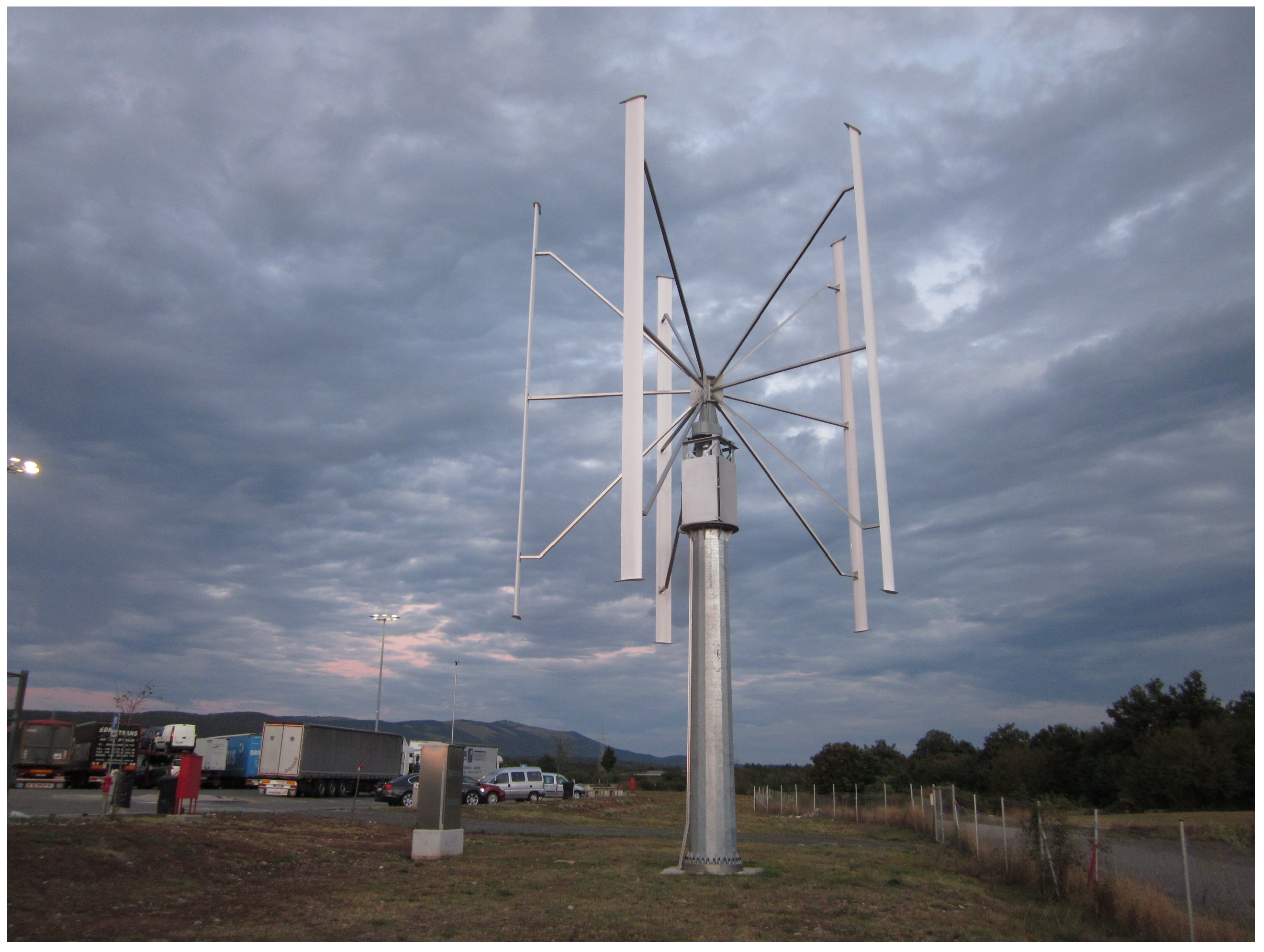
Small wind turbines (Figure 1), which are defined as turbines with rotor swept area under 200 m${}^2$ and generating electricity below a certain voltage [1], are popular and being installed at an increasing rate [2,3,4,5]. The wind characteristics at the site of a wind turbine have a big influence on its performance [6,7] and noise emissions [8]. Thus, it is important to select a good site for placing it.

The standard method for evaluating a candidate site for a wind turbine is collecting long-term wind measurements at the site. The decision on whether to install a wind turbine at a particular location is most often based on the annual energy production, which can be estimated from the wind speed distribution and the wind turbine power curve [9,10,11]. The measurement taking time and delaying the decision process is the issue addressed in this work.

The motivation for this investigation is avoiding the long wait for wind measurements from the candidate turbine site to be collected. A method for the fast evaluation of the feasibility of a site for the possible placement of a wind turbine is developed and tested. The method predicts the yearly time series of the wind speed at the site and derives the wind speed distribution from it. The distribution is more important than the time series, because it is related to the annual energy production. The presented method would be easy to use at different sites without requiring additional research—the goal is for the application of the method to fit the budget of a small wind turbine construction.

The assumed situation that is being addressed is the following:

• Because of time constraints, one month of wind speed measurements from the candidate turbine site is available.
• A fine resolution numerical weather prediction (NWP) model for the area is available and its predictions for the past are available.
• Past measurements from meteorological stations in the area, but not from the site under examination, are available.
• One year of wind speed and direction signals for the candidate site are sought after, so 11 months are predicted.
• A yes/no decision on installing the wind turbine at the exact location is required—the option of adjusting the location is not considered.

For clarification of the further notation, signal is a time-dependent physical quantity that carries information regarding the system. It can be either measured on the real system or obtained as an output of a model. System is the atmosphere and the other parts of the environment that influence the weather, and model is a numerical approximation of the system.

Shortening the measurement period involves risks that are proportional to the size of the project. Therefore, it is particularly tempting to use an alternative and less accurate site evaluation method if the wind turbine is small. One possible alternative would be using NWP-predicted signals as a proxy for local wind speed, even though NWP models, such as Weather Research and Forecasting model (WRF), do not reflect local terrain effects as they represent values ascribed to staggered grid points [12]. Furthermore, unlike big wind turbines, small ones may be used at low heights above ground and in areas with low average wind speed, where NWP is particularly inaccurate in predicting local wind speed. Because of these reasons, the presented method is likely to be especially suitable for evaluating sites for small wind turbines.

The goals are achieved with a novel approach in this field—system identification. An experimental model (i.e., a mathematical model that is based on measurement data) is trained with a short time series of training data, one month in our case. The output of the model is the wind speed at the candidate turbine site, which only has to be measured during the training period. The inputs of the model are the signals that are available for the past independently from the wind project— measurements from the meteorological stations in the vicinity and NWP signals. The trained model is then used as a soft sensor. It predicts the wind signal for a longer past period in which the wind speed at the site was not measured, but during which the model inputs are available.

To evaluate the feasibility of such use of modelling, model predictions are compared to the measurements over a test period, which is separate from the training period. Several methods of linear and nonlinear modelling are tested and their suitability for the purpose is evaluated. The test locations are in a complex terrain with moderate winds. This is desirable, because models for such sites are needed—near-future turbine technology will allow harvesting of wind energy over low wind regions at wind speeds as low as 3 $\mathrm{m}/\mathrm{s}$ [13]. Models have rarely addressed such areas because wind power forecasting has more often been used in flat terrain with strong persistent winds. Modelling a complex terrain is also a challenging test for the modelling method, which is beneficial.

The requirements in candidate wind turbine site evaluation are somewhat different than in either wind power forecasting or in wind resource assessment. Recent wind power forecasting research "can predict the fluctuation of output wind power in wind farms” [14] and, therefore, helps to ensure safe operation of the power system [15]. Multi step forecast is achieved by singular spectrum analysis and a hybrid Laguerre neural network [14] or based on extreme learning machine in multi-objective optimization algorithm [16] or Convolutional Neural Network cascaded with a Radial Basis Function Neural Network [17].

The task of predicting local wind signals from other signals with a limited amount of training data introduces different constraints than wind power forecasting modelling:

• The prediction is not real-time, eliminating the timing constraints—model inputs do not have to be available before the time for which the prediction is made. Reanalyses, which are more accurate, can be used.
• No measurement of the wind parameters on the candidate site is available as a model input. The measurements are available as training data to train the model, but not as an input at times close to the time for which the prediction is made.

The wind resource assessment models give the answer on the energy yields in the region under examination. Over complex terrain, the results of mesoscale numerical weather prediction model WRF can fulfill this need [18]. Wind resource assessment models with fine spatial resolution can solve the problem of optimal siting of turbines within a wind farm, while taking the interactions among the turbines and with complex terrains into account [19]. To achieve the same goal of increasing energy yields, measurements from several masts can be coupled using computational fluid dynamics [20].

The proposed models for evaluating a candidate site differ from the wind resource assessment models in the following aspects:

• The available data cover a very limited time period.
• The focus is on a single location.
• There is a lack of time for measuring, while the wind resource assessment models are addressing the lack of measurement sites in spatial dimensions.

Table 1. Requirements for fulfilling different needs in wind power. Wind resource assessment characterizes the resource over an area, is performed on historical data, and has long-term time series data available at most for a limited set of locations in the area. Wind power forecasting addresses a selected site, has to work in real time, and it has real-time measurements from the site available. Evaluating a candidate site is done for a selected site on historical data. Traditionally, it requires long-term time series measurement data from the site, while the proposed method performs it with a shorter-term time series of measurements from the site, supported with other available signals.

Addressed Need	Location?	Real-Time Output or Historic Data?	Local Measurements?
Wind resource assessment	area	historic	spatially limited
Wind power forecasting	point	real-time	available
Candidate site evaluation	point	historic	available *

* The proposed solution enables evaluation with temporally limited local measurements.

summarizes the requirements of candidate site evaluation, wind power forecasting, and wind resource assessment.

The novel contribution of the presented work is the method how experimental modelling of wind speed time series is used to help with decisions on small wind turbine placement in complex terrain. To our knowledge, there have been no prior attempts to use a shorter measurement time series and compensate for it using modelling. The classical approach is collecting a long-term time series of wind measurements at the site and basing the decisions on these measurements. The drawback is the wait for the measurements to be collected. The proposed solution avoids the wait through measuring for a shorter period and using the collected measurements to train a model that is then able to predict the wind speed at the site for a longer period in the past. The model predictions can inform the turbine placement decisions, provided that they are close enough to the real wind speed values. Several different linear and nonlinear modelling methods are used, and results they provide are evaluated.

Even though the wind speed is available as a NWP grid cell variable, experimental modelling is necessary to obtain its local value, because NWP discretization is coarse as compared to the length scale of interest. The use of modelling to obtain local weather variables from NWP predictions is established and it is called model output statistics (MOS) [21]. MOS has been successfully used for wind power forecasting and nowcasting [22,23,24] and for wind resource assessment [25,26,27], but not for site evaluation. When compared to typical MOS studies, the original contributions of the manuscript are the use of short training data sets, improving MOS through the use of measurements from the meteorological stations in the vicinity, and evaluation of the results from the perspective of wind turbine placement by emphasizing the predicted wind speed distribution. The shortness of the training data sets reflects the fact that the time used for data collection delays the subsequent stages of the project. The work is significant, since wind power, including small wind turbines, is popular and the work proposes a way for shortening the delay between the start of measuring and the turbine installation. No similar solution seems to have been suggested before.

The proposed method is better suited for small wind turbines than for large ones for several reasons. Small wind turbines tend to be installed in places with low wind speeds [28], especially in off-grid applications [29], and at smaller heights. NWP signals predict the wind speed at these locations less accurately than high above a flatter, windier terrain. While large wind turbines may be located in a wind farm and distributed so as to optimally use the available area, economic reasons, such as land ownership, are likely to limit a small wind turbine to an exact location, aligning it with the assumptions of the method. In addition, it is easier to envisage making the decision to build a wind turbine based on a short period of local wind measurements when the turbine in question is small.

Crucially for future practical application of the work, the proposed experimental modelling method is easy to use and no special modelling skills are required for utilizing it (the best performance is achieved with the most usual linear regression fitted with least squares using a few straightforward independent variables). Thus, its use would fit into the small planning budget for a small wind turbine.

2. Methods

Wind time series at a meteorological station that represents a candidate wind turbine location is modelled. As model inputs, measurements from the meteorological stations in the vicinity and NWP model outputs are used. A single calendar month of training data is used, the process is repeated through the whole year, and a separate model is generated for each training month. Thus, each one of the 12 models obtained is tested on the remaining 11 months of the measurement data that are not used in training. Several different linear and nonlinear modelling methods are examined. They are evaluated graphically and using figures of merit. Some plots and figures of merit are dedicated to comparing the measured and predicted wind speed distributions, as they are particularly important in wind power.

2.1. Description of the Site

The study area comprises the Krško Basin and the surrounding hills. Figure 2 provides a panoramic view, and Figure 3 shows the topography. The climate is temperate humid with warm summers [30,31]. The land use is diverse—urban, fields, forests, water bodies, etc.—as demonstrated by CORINE Land Cover 2018 Version 20 data [32] and shown in Figure 4.

A NWP model for the area that is based on WRF-ARV version 3.4.1 [12] with 4 km horizontal resolution is available [33,34]. Weather Research and Forecasting model (WRF) is one of the best currently available mesoscale NWP models. It is suitable for weather forecasting over complex terrain in fine spatial and temporal resolution. Its outputs are time series of wind, temperature, and other meteorological variables as ground level values and vertical profiles on selected grid locations. WRF-ARW is Advanced Research WRF, one of the two available versions of WRF.

The study uses data from four meteorological stations, as listed in

Table 2. Locations of meteorological stations.

Name	WGS84 Coordinates
	Latitude	Longitude
Brežice	45.906760	15.596502
Cerklje Airport	45.900833	15.516111
Lisca	46.067735	15.284905
Stolp	45.939900	15.513132

. The station Brežice represents a candidate site for small wind turbine placement in most of the numerical experiments, while signals from the other three are used as model inputs. The ground level wind signals are measured at 10 m height at all of the stations. The meteorological stations are up to 30 km apart.

2.2. Signals

All of the measured and NWP-generated meteorological signals are recorded every 30 min. In the case of measured quantities, 30 min. averages are recorded. Averages with shorter sampling times are not available. There are seven NWP signals available—wind speed and direction, temperature, humidity, air pressure, cloud cover, and global solar radiation—while one additional signal, diffuse solar radiation is derived from NWP signals using an artificial neural network [35,36]. Diffuse solar radiation is the part of solar radiation that is reflected from clouds or other objects, dispersed in the fog, etc. It is not easily predicted over complex terrain, therefore a dedicated model of it is used.

Three standard ground level meteorological stations in the vicinity are available, measuring 26 signals in total, and the wind measurement is taken 10 m above ground. The signals for the calendar year 2017 are used.

2.3. Regressors

Regressors are the independent variables that the model output depends on. They are selected or computed from the available input signals. Their choice is based on the general meteorological knowledge and on the familiarity with the area. The four regressors used are:

• the current wind speed at Cerklje Airport meteorological station;
• the current wind speed according to the NWP model;
• the current temperature difference between Lisca and Cerklje Airport meteorological stations; and,
• the air pressure change in the last 2 h at Stolp meteorological station.

A good source of information for predicting the wind speed at the studied location is the measured wind speed at a nearby meteorological station, used as regressor 1. Another one is the wind that is predicted by the NWP model for the local cell of the studied site, used as regressor 2. Regressor 3, the temperature difference between two meteorological stations at different altitudes, is proportional to the vertical temperature gradient and, thus, to the atmospheric stability. Changes in the air pressure drive the weather, which is the reason for choosing regressor 4. The differences used as regressors 3 and 4 are less dependent on the season than absolute air pressure and temperature values. This makes them a good choice for a model that is trained on a single month and used throughout the year.

Quantitative algorithms for regressor selection also exist [37], and they could have been used as an alternative to the presented heuristic method. The quantitative algorithms are universal, they can be applied to any signals, and require no knowledge of the modelled system. However, their use requires skill and, in some cases, a lot of computing time.

2.4. Linear Regression

Linear regression, fitted with least squares, is the basic linear approach in modelling the relationship between the regressors and output variable. It is used to derive 24 of the 60 presented models.

2.5. Gaussian Process Modelling

As the mathematical structure of the model describing the relationship between the regressors and the output variable, a Gaussian process (Gaussian process should not be confused with other terms named after Gauss, such as Gaussian diffusion models in atmospheric dispersion modelling) (GP) is used in 36 of the 60 presented examples. GP models are typically nonlinear. Unlike the other nonlinear models, the GP models provide model uncertainty through variance prediction, which is their main advantage and the reason they are used in this study.

GP is a stochastic process $f\left(\mathbf{z}\right)$ for which any finite set of function values is jointly normally distributed [37],

$$p\left(f\left({\mathbf{z}}_1\right),\dots ,f\left({\mathbf{z}}_M\right)|{\mathbf{z}}_1,\dots ,{\mathbf{z}}_M\right)=\mathcal{N}\left(\mathbf{m},\Sigma \right).$$

(1)

In GP modelling, a covariance function or kernel function k is used to obtain the covariance matrix elements as ${\Sigma }_{ij}=k\left({\mathbf{z}}_i,{\mathbf{z}}_j\right)$, while $\mathbf{m}$ is set to $\mathbf{m}=0$. The model output distribution for a given input is obtained from a joint distribution $\mathcal{N}$ with the training data. Unless k is a linear function, GP models are, in general, nonlinear.

The model output is treated as noisy with uncorrelated Gaussian measurement noise, the variance of which is independent of the model input. The covariance function encodes the assumptions about the modelled system [38]. Typically, the covariance function is not fully prescribed in advance, but has some free parameters, named hyperparameters. Their values are chosen together with the value for the noise variance so as to maximize their likelihood given the training data [37].

2.6. Experimental Modelling

As different experimental modelling methods have different strengths, several of them are used for predicting the wind speed:

GP SE:

Gaussian process model with squared exponential covariance function;

GP lin:

Gaussian process model with linear covariance function;

GP SE+lin:

Gaussian process model with covariance function that is the sum of a squared exponential function and a linear function; and,

LS lin:

linear regression with least squares approximation.

GP SE and GP SE+lin are general purpose nonlinear modelling methods. GP lin and LS lin result in different linear models. The implementation of GP SE, GP lin, and GP SE+lin is as described in Section 2.5, while the linear regression of LS lin is implemented in MATLAB Statistics and Machine Learning Toolbox functions.

The difference between GP lin and LS lin is in the assumed measurement noise distribution. The least squares method results in the best possible fit as long as the output error is Gaussian, while the Gaussian process linear model makes no such assumption in maximizing the likelihood.

All of the models share the Finite impulse response (FIR) [37] structure, as there are no delayed output values in the regressor list. FIR structure is chosen because it avoids error propagation issues of Autoregressive models with exogenous input, resulting in faster computation and enabling us to do more extensive testing. A drawback of FIR models is that they typically require many delayed values of input signals to achieve good results. However, the results of the numerical experiments show that this is not the case in our example. The finding is in agreement with the physical background of the system.

The training data for each model are the data for one of the 12 months in the year. Each model is tested through predicting the output variable for the 11 months of the year not used in training. A separate model is made using each one of the 12 months as the training month, which results in 12 tested models for each modelling method, as depicted in Figure 5.

2.7. Model Evaluation

The models are qualitatively evaluated using various relevant plots and quantitatively using figures of merit. Quantitative evaluation is more exact, more convenient for ranking the models, and based on the whole dataset, while qualitative evaluation is more profound and it better illustrates the behaviour of the model. Thus, it is beneficial to use both. For qualitative evaluation, time series plots, scatter plots, Q–Q plots, and sunflower diagrams [39] are used, while quantitative evaluation is based on several different figures of merit.

In accordance with the assumption that only one month of data is available for construction of the model, the signals of the 11-month test period are not used at any stage of modelling. Thus, the test data set used in model evaluation is completely independent.

2.7.1. Qualitative

Tme series of the predicted and of the measured signal are plotted to qualitatively observe the models’ response.

Scatter plots emphasise the relationship between the measured value at a given time and the model output at the same time. This is achieved by omitting the time dependence of the signals.

The distributions of the predicted and measured wind speeds are best compared with Q–Q plots. The values plot on the line of equality if the distributions are equal and the deviations from the line mark the parts of the distribution that differ.

The sunflower diagrams reveal the information on the wind speed distribution at different times of day. This is particularly useful if the energy production at different times of day is of interest, e.g., if the electric energy price varies throughout the day.

2.7.2. Quantitative

Figures of merit enable us to quantitatively evaluate the results of the wind speed models for wind resource characterization and to benchmark the experimental models against NWP.

Pearson correlation coefficient R, coefficient of determination R${}^2$, mean square error (MSE), and mean standardised log loss (MSLL) values are used in evaluating the results of the models.

Pearson correlation coefficient is defined as

$$\mathrm{R}=\frac{\mathrm{cov}(\mathbf{y},\mu )}{{\sigma }_{\mathbf{y}}{\sigma }_{\mu }},$$

(2)

where $\mathbf{y}$ is the vector of measured values, $\mu$ is the vector of predicted values, cov is covariance, ${\sigma }_{\mathbf{y}}$ is the standard deviation of the measured value, and ${\sigma }_{\mu }$ is the standard deviation of the predicted (mean) value. The value is between −1 and 1, and the more positive value is better.

The coefficient of determination is defined as

$${\mathrm{R}}^2=1-\frac{{∥\mathbf{y}-\mu ∥}^2}{N{\sigma }_{\mathbf{y}}^2},$$

(3)

where N is the number of the test samples and ${\sigma }_{\mathbf{y}}^2$ is the variance of the measured value. The value is between 0 and 1, and a bigger value is better.

MSE is defined as

$$\mathrm{MSE}=\frac{{∥\mathbf{y}-\mu ∥}^2}{N};$$

(4)

It is always positive and smaller is better.

MSLL is defined as [38]

$$\mathrm{MSLL}=\frac{1}{2N}\sum _{i=1}^N\left[ln\left({\sigma }_i^2\right)-ln\left({\sigma }_{\mathbf{y}}^2\right)+\frac{{\left(E\left({\widehat{y}}_i\right)-y_i\right)}^2}{{\sigma }_i^2}-\frac{{\left(y_i-E\left(\mathbf{y}\right)\right)}^2}{{\sigma }_{\mathbf{y}}^2}\right],$$

(5)

where $y_i$ is the measured value, $E\left({\widehat{y}}_i\right)$ is the mean prediction, and ${\sigma }_i^2$ is the predictive variance. The summation includes all of the test samples and the index i corresponds to the sample. MSLL takes the predictive variance into account. A lower MSLL value corresponds to a better model, and the values are typically negative.

R, R${}^2$, and MSE are popular standard figures of merit. They do not provide completely independent information, and the main reason for listing several of them is for easier comparison with other studies. MSLL is the figure of merit that is used to evaluate the predictive variance in addition to the predicted mean value.

To evaluate the time-series results over the whole sample of the models, the figure of merit for each modelling method is averaged over the 12 models that were obtained with different training months.

Estimating the annual energy production or related derivatives from the wind speed distribution is specific to the turbine [9] and is not attempted. The average wind speed $\overline{v}$ and the average cube of the wind speed $\overline{v^3}$, averaged over time throughout the test period, are used to quantify the distributions instead. The model-predicted values of $\overline{v}$ and $\overline{v^3}$ are computed from the predicted expected values of the wind speed. They are compared to the values of $\overline{v}$ and $\overline{v^3}$ that are calculated from the field measurements over the same period. For each modelling method, the MSE of either quantity over the 12 different choices of the training month is computed.

2.8. Spatial Transferability of the Method

The model structure and the regressors are chosen based on the whole region and not adapted to a particular location. Thus, the model is only bound to a specific location by the training output signal of wind speed measurements. If the wind measurements for the training are taken at another location within the region, the resulting model will be valid for the new location. This is demonstrated by modelling the wind speed at Stolp meteorological station, which is over 7 km away from Brežice, and it has very different surroundings and wind speeds.

3. Results

The results that are directly related to the predicted wind speed time series are presented separately from the ones related to the wind speed distributions of the predictions.

3.1. Time-Series Modelling Results

Figure 6 and Figure 7 set the measured signal of wind speed at Brežice meteorological station side-by-side with the predictions of one of the models. It can be seen that there is a match between the measurement and the prediction.

Table 3. Figures of merit for various models of wind speed at Brežice meteorological station and for LS lin model at Stolp meteorological station. The values given are the values obtained on the test data averaged over the 12 models with different train/test data set selections and the Brežice models are ordered in ascending MSE.

Model Name	R	R${}^2$	MSE [m${}^2$/s${}^2$]	MSLL
LS lin	0.685	0.454	0.243	−0.285
GP lin	0.685	0.435	0.251	−0.266
GP SE+lin	0.636	0.378	0.276	−0.198
GP SE	0.601	0.341	0.293	−0.190
NWP	0.418	0.000	2.842	-
LS lin Stolp	0.811	0.652	0.442	−0.514

shows the figures of merit for various modelling methods of wind speed. The values are averages: each modelling method is used on 12 different training months. Each model is tested on the remaining 11 months of the data. The 12 test figures of merit are averaged. It can be seen that, in terms of these two figures of merit, LS lin models perform best at the Brežice meteorological station. If raw NWP values are used to approximate the local wind speed, they perform very poorly.

At Stolp meteorological station, the best-performing modelling method, which is, LS lin, is used. The dimensionless figures of merit show that modelling of the wind speed at Stolp is more successful than at Brežice. The likely explanation is that Stolp is the better positioned meteorological station of the two with less local obstacles. The MSE values should not be directly compared between the two locations, as winds at Stolp are, on average, 38% faster than at Brežice.

3.2. Results Related to Wind Speed Distribution

The role of the MSE($\overline{v}$) value is comparing the average wind speed during the 11 month test period as predicted by the models with the actual average wind speed. Each modelling method results in 12 average wind speeds, and

Table 4. Wind speed distribution-related figures of merit for various models of wind speed at Brežice meteorological station and for LS lin model at Stolp meteorological station. The wind speed and the cube of the wind speed are averaged over the 11-month test period for each model to obtain $\overline{v}$ and $\overline{v^3}$. The difference between $\overline{v}$ or $\overline{v^3}$ obtained with model prediction and $\overline{v}$ or $\overline{v^3}$ obtained from the measurement is computed, squared, and the 12 squares that correspond to the 12 train/test data set selections are averaged.

Model Name	MSE($\overline{\mathit{v}}$) [m${}^2$/s${}^2$]	MSE($\overline{{\mathit{v}}^3}$) [m${}^6$/s${}^6$]
LS lin	0.003	1.177
GP lin	0.011	1.399
GP SE+lin	0.005	1.210
GP SE	0.004	1.421
NWP	1.004	645.327
LS lin Stolp	0.003	14.179

provides the MSE of these results. The third power of the wind speed is likewise averaged and its MSE is presented in the column MSE($\overline{v^3}$). The models that better predict the wind speed time series (see Table 3) tend to also predict average values that are closer to the true average.

Predictions of one of the LS lin models from each site are statistically compared to the measured wind speeds and NWP predictions in Figure 8, Figure 9 and Figure 10. Scatter plots, Q–Q plots, and sunflower diagrams showing the daily wind patterns are presented. The shown LS lin model is the one with the choice of the training month that resulted in the best MSE at each site.

4. Discussion

Decisions regarding small wind turbine placement benefit a lot from obtaining more useful information from a shorter period of data measured at a candidate location. A way of achieving this goal is by using the measurement data of the wind speed to train a model of this quantity with inputs that are available for a longer time period, such as NWP signals and measurements from the meteorological stations in the vicinity. Several experimental models for the purpose that use these signals and their combinations as regressors are proposed and tested.

In testing, the criteria for model quality have to be defined in a meaningful way. The match between the measurement and the model is shown in Figure 6 and Figure 7 and in the scatter plots in Figure 8 and Figure 9, and Table 3 lists the standard figures of merit. These pieces of information offer a general measure on model performance, which is useful in developing and improving the models. However, they do not directly address the performance of the models in wind turbine placement decisions. These decisions are based on wind statistics [40] the choice of which depends on the type of the turbine and even on the turbine use case—one is typically, but not necessarily, interested in the annual energy production. The local wind predicted by the model has to result in similar values of the chosen statistics if the model is to be useful in decision-making.

To this end, the measured and predicted wind speed distributions are compared in Q–Q plots and sunflower diagrams in Figure 8, Figure 9 and Figure 10. We see that the distributions that are predicted by the linear regression with least squares models match the distributions of measured values better than the NWP model does. The match is quite good, particularly for speeds under 5 m/s. Beyond that point, the mismatch in Q–Q plots increases, while the frequency of the speeds decreases. Figure 10 demonstrates that the predicted and measured speed distributions match by hour of day. This is beneficial if one is interested in the dependence of power on time and it is also a confirmation of the skill of the model. A couple of meaningful statistics from the model results are calculated—the average wind speed $\overline{v}$ and the average wind speed to the third power $\overline{v^3}$. The reason for choosing $\overline{v}$ is that it is the simplest wind speed statistic that is related to wind power. Wind power by unit area is proportional to $v^3$ [40], so its average is also examined. The results in Table 4 show that the models better matching the measurements are also better at predicting $\overline{v}$ and $\overline{v^3}$. This indicates that the good predictions of the wind speed distributions and of the $\overline{v}$ and $\overline{v^3}$ values result from successful time-series modelling and can be relied on.

The measured wind speeds at the studied locations are below the typical necessary speeds for wind power use. However, they are within the expected range of wind speeds for a candidate site, as it is, by definition, not possible to avoid infeasible locations when doing feasibility studies. The locations are thus adequate for testing of the presented method—for models used in checking feasibility, it is, in fact, most important that they perform well close to the boundary of feasibility. At the same time, the location-optimized design of wind turbines is becoming more common, enabling wind power use, even at these speeds [41]. The required wind speed for a viable wind farm is also lower when sustainable development is taken into account than if only financial value is considered [42].

The NWP signals used are generated with the finest resolution NWP model that is available for the study area. The use of the best available data improves the chances of success, which is desirable for the initial testing of a novel method. It is not implied that the method would not work with a coarser NWP grid, especially on a flatter terrain, but it remains to be tested.

It is assumed that the training wind measurements at the candidate site are collected at the target height for the turbine. In the presented case, the height is 10 m, which is within the range for small wind turbines (Figure 1). As 10 m is the standard for meteorological stations, the wind measurements at the surrounding stations that are used as model inputs are measured at the same height. However, this is not a requirement. The training wind measurements at the location should be taken at the planned turbine height, but the wind measurements from the meteorological stations in the vicinity can be used as model inputs, regardless of the height at which they are taken.

The presented use case precludes collecting measurements at different times of the year, because avoiding year-long measurements is the objective of the modelling. As the model is to be used year-round, the training data only span a part of the operating range in which the model is to be used, which is undesirable. The observed good performance of the model can be ascribed to the careful selection of the regressors. The temperature difference between two locations at different altitudes is less seasonal than the temperature itself. Similarly, the air pressure change over a given time period is less affected by the season than the air pressure itself. The remaining two regressors are wind speeds at a nearby location and as predicted by the NWP model. The dependence of the model output on these two seems to be close enough to linear that it is identified sufficiently well by the used linear model from the limited training data available. Models of this kind have the potential to also work in other areas, particularly in areas similar to the studied one. Nevertheless, when applying the method to a new region, it may be beneficial to validate a model on the data from an established meteorological station before using it for wind turbine placement decisions, particularly if the region is very different in climate or topography from the one studied here.

The finding that least-squares linear regression models perform well is fortunate for the possible practical use of the model. The most laborious part of the modelling process is selecting the potential regressors and obtaining and parsing the historical data, which is likely to have been done in the earlier stages of the project. Coding the model in a high-level computer language is trivial and the required computation time is under a second. The processing of the model output is no different from processing a long-term measured time series, which would be required otherwise. thus, such modelling is completely feasible, even in the scope of a small wind power project.

5. Conclusions

A method for evaluating wind conditions at candidate locations for small wind turbine installation with short time series of local measurement data is developed. Different soft sensors of the wind speed at the studied locations are constructed, tested, and compared. They use measurements from the meteorological stations in the vicinity and numerical weather prediction signals as inputs.

The tested soft sensors predict the wind speed time series well and the wind speed distribution very well. The predictions of the soft sensors are much better when compared to the predictions of the high resolution NWP model. A linear model optimized with least squares performs better than the tested nonlinear models in predicting the wind speed at the main study site.

The proposed modelling method can serve to shorten the wait for the measurements when evaluating candidate locations for small wind turbines, which enables the turbine to be built more quickly and to start producing electricity sooner. It is conceptually simple and easy to use, so it is practical to apply, even when planning the installation and operation of a small wind turbine where the budget does not allow for expensive studies.

The envisioned use of the method only assigns a short part of the year for taking measurements. Thus, the resulting experimental model has to be trained on data points covering only a part of the range of conditions in which the model is going to be used. The theory of system identification does not recommend such extrapolation, as it can harm the model performance. Fortunately, the presented models give good predictions, regardless of it. Part of the reason may be in careful choice of meaningful regressors. Linear models tend to perform relatively well in extrapolation, which may explain why the linear models have the best performance.

The method is likely to work similarly well in different regions if the regressors are chosen so as to provide similar information than the ones that are used in the study. However, the good performance of the models is not completely explained and expected, so equally good results in areas very different from the study area cannot be guaranteed. It should be noted that the same regressors result in good models for different sites in the study area. When using it in another area, the method, including the choice of regressors, can first be validated on sites with the historical data available and then applied to the candidate wind turbine sites.

Two directions of future research are proposed. Verifying that the findings generalize to different climates and topographies is one of the objectives, which will enable the method to be used in a wider geographic range. In addition, the method is ready to be tested in actual candidate wind turbine locations, particularly in complex terrain in temperate regions.