Article

Network Analysis to Identify the Risk of Epidemic Spreading

1
Department of Bio and Brain Engineering, KAIST, Daejeon 34141, Korea
2
R&D Center, BioBrain Inc., Daejeon 34141, Korea
3
Department of ICT Convergence System Engineering, Chonnam National University, Gwangju 61005, Korea
4
Bio-Synergy Research Center, Daejeon 34141, Korea
5
Moon Soul Graduate School of Future Strategy, KAIST, Daejeon 34141, Korea
*
Authors to whom correspondence should be addressed.
Co-first author, these authors contributed equally to this work.
Appl. Sci. 2021, 11(7), 2997; https://doi.org/10.3390/app11072997
Submission received: 24 February 2021 / Revised: 15 March 2021 / Accepted: 24 March 2021 / Published: 26 March 2021
(This article belongs to the Section Environmental Sciences)

Abstract

:
Several epidemics, such as the Black Death and the Spanish flu, have threatened human life throughout history; however, it is unclear if humans will remain safe from the sudden and fast spread of epidemic diseases. Moreover, the transmission characteristics of epidemics remain undiscovered. In this study, we present the results of an epidemic simulation experiment revealing the relationship between epidemic parameters and pandemic risk. To analyze the time-dependent risk and impact of epidemics, we considered two parameters for infectious diseases: the recovery time from infection and the transmission rate of the disease. Based on the epidemic simulation, we identified two important aspects of human safety with regard to the threat of a pandemic. First, humans should be safe if the fatality rate is below 100%. Second, even when the fatality rate is 100%, humans would be safe if the average degree of human social networks is below a threshold value. Nevertheless, certain diseases can potentially infect all nodes in the human social networks, and these diseases cause a pandemic when the average degree is larger than the threshold value. These results indicated that certain infectious diseases lead to human extinction and can be prevented by minimizing human contact.

1. Introduction

The emergence of a pandemic is one of the various scenarios frequently discussed as a human extinction event, and it is listed as one of the global catastrophic risks in studies regarding the future [1,2,3]. In particular, several pandemics, such as the Black Death [4,5], Spanish flu [6], and those caused by smallpox [7], severe acute respiratory syndrome (SARS) [8], and Ebola [9], have affected a large population throughout history. The risk of pandemics increases with an increase in population mobility between cities, nations, and continents, thereby threatening humankind [10,11,12]. It is essential to analyze the epidemic spread in society to minimize the damage from epidemic disasters; however, extinctive epidemic spreading experiments have limitations in real-world situations, as they predict stochastic effects on the spread without considering the structure of human society. Network-based approaches have been proposed to overcome these limitations and perform epidemic spreading simulations by considering the network structure of numerous real-world connections [13,14,15]. These methods use various models of epidemic spreading, such as the susceptible–infectious–susceptible (SIS) [16,17,18], susceptible–infectious–recovered (SIR) [19,20,21], and Watts threshold models [22]. While these methods are mathematically convenient, they are epidemiologically unrealistic for various infections because they require exponentially distributed incubation and infectious periods [23,24,25]. Moreover, previous epidemic studies did not perform quantitative assessment of the pandemic risk depending on the network connectivity in individuals and fatality rate of various diseases [26].
In the present study, we applied an SIR epidemic model to a scale-free network with Monte Carlo simulation to identify the quantitative relationship between infectious diseases and human existence. Our fundamental hypothesis states that when the epidemic spreads to all nodes of the network and the fatality rate is 100%, it can increase the pandemic risk. To address this, we initially constructed a scale-free network to simulate a society. Moreover, for the epidemic spreading simulation, an SIR model was applied to the network to describe the immune state of an individual after infection. From the simulation study, we found that the mean degree of a scale-free network was an essential factor in determining whether epidemics threaten humans. This approach provides important insights into epidemic spreading analysis by investigating the relationship between epidemic and scale-free network parameters. Furthermore, it highlights the necessity of determining information flow during an epidemic.

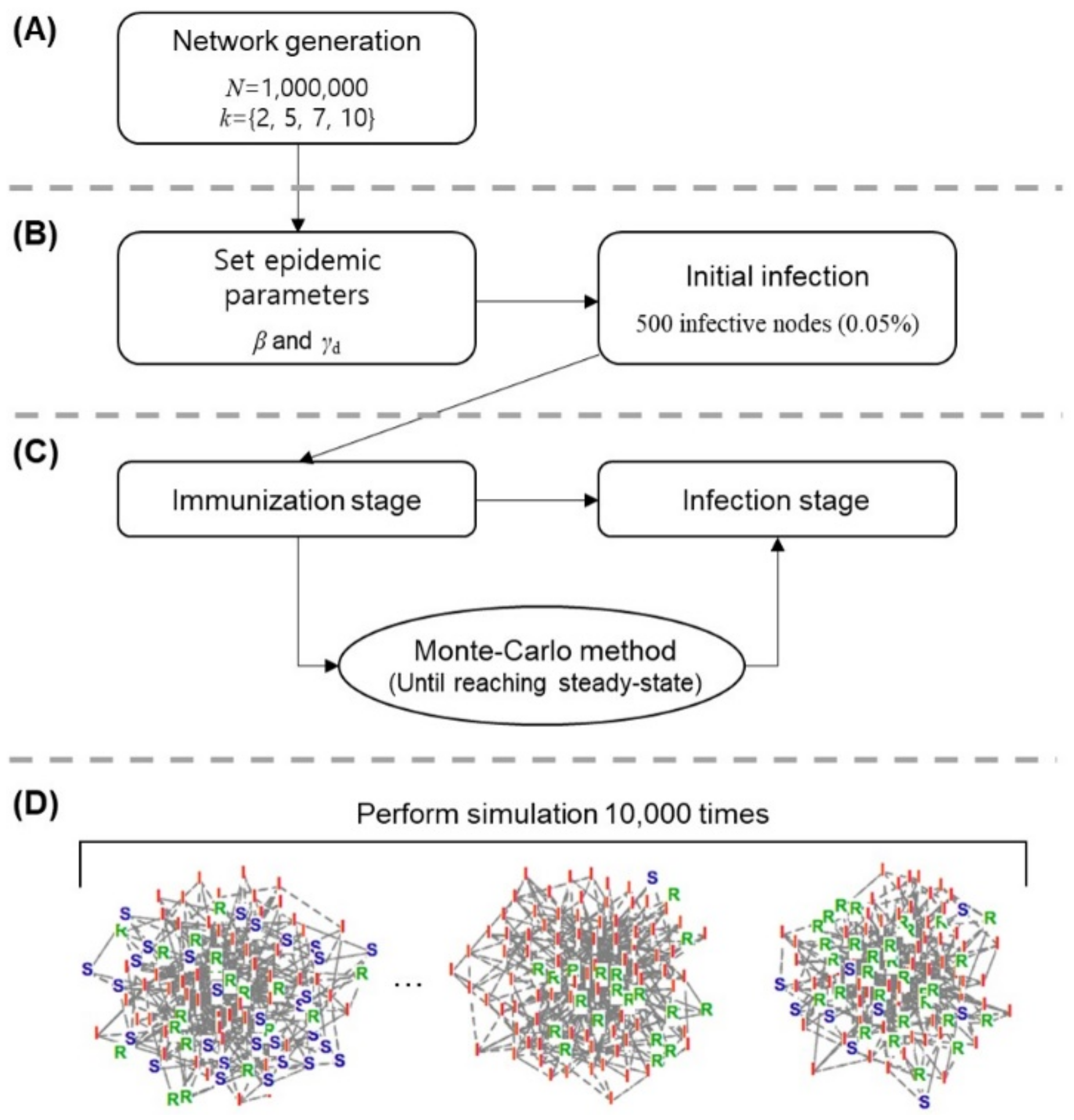
2. Materials and Methods

We designed an epidemic simulation process to identify the relationship between pandemic risk and network parameters. This study was performed in four steps (Figure 1): (i) generating a scale-free network model to reflect real-world conditions; (ii) applying an SIR model to the scale-free network for epidemic spreading simulations; (iii) adapting the Monte Carlo method to reflect the stochastic process in the node status of the SIR model; and (iv) iteratively performing simulation for every parameter set and analyzing the results. We have provided the source code and sample results of epidemic simulation in Supplementary Materials.

2.1. Network Generation Based on a Scale-Free Model

We constructed a network model for the epidemic spreading simulation (Figure 1). The nodes and edges of the network represent people in the society and their physical contacts, respectively. We used a scale-free network model, which follows the preferential attachment property observed in numerous real-world networks, such as social networks, physical systems, and economic networks [27,28,29]. In the scale-free network, when a node is added to the network, its likelihood of connecting to existing nodes increases with an increase in the node’s degree. Hub nodes, which lead to fast and vast spreading of epidemics, exist. Two characteristic parameters, including N and k, affect the form of scale-free networks. The parameter N denotes all nodes in the network. In the real world, N indicates the whole population size. The parameter k is the average degree of the network, which determines the degree of the newly attached node for each step during network generation. Following the characteristics of the network model, we generated scale-free networks representing human contacts for epidemic spread. The scale-free network was generated by the Barabasi–Albert graph distribution, in which the network is constructed from a cycle graph with three vertices, followed by the addition of k edges at each construction step [30]. The k edges are randomly attached to the vertex based on the degree distribution of the vertex. After network generation, we investigated the degree distribution properties of the network (Figure 2). The results indicate that the degree distributions have similar tendency for networks with varying number of nodes and edges. This study constructed scale-free networks with the largest number of nodes considering computational complexity (N = 1,000,000).

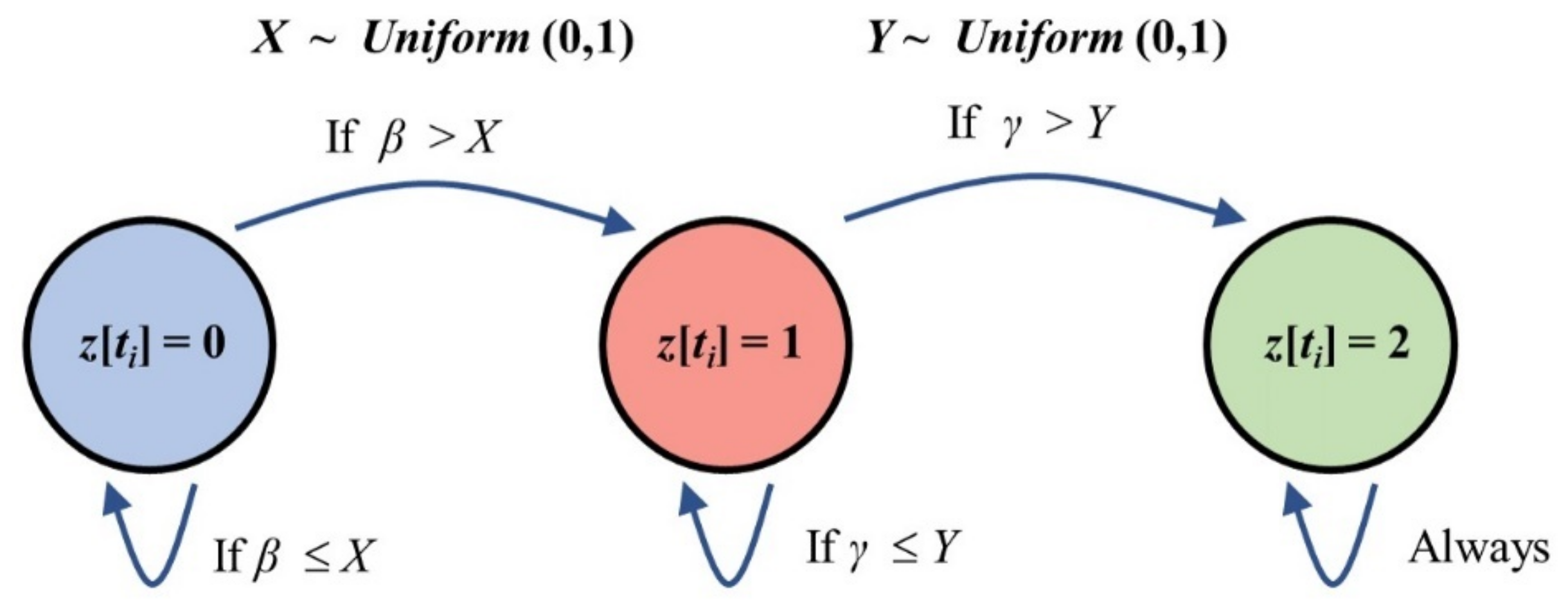
2.2. Epidemic Spreading Based on the SIR Model

For the epidemic spreading simulations, we applied an SIR model to the generated scale-free network. The classical SIR model can be expressed by the following nonlinear differential equations [21]:
d S d t = β S I ,
d I d t = β S I γ I ,
d R d t = γ I ,
S + I + R = N,
where S, I, and R represent susceptible, infected, and recovered compartments, respectively, in the whole population. S represents people who have not been infected yet but can be infected in future. I represents infected people who can spread the epidemic to susceptible people through physical contact. R denotes people who have recovered or died from the epidemic and who no longer participate in the epidemic spreading process. The sum of the S, I, and R values represents the whole population size N. Epidemics have two parameters in the SIR model, transmission rate (β) and recovery rate (γ), which arise from the basic reproduction number R0 (Figure 1B). The basic reproduction number is the number of infections caused by one infective node [31,32,33]. If the R0 is more than 1, the infection can spread in a population, whereas if R0 is less than 1, the infection cannot spread. We express the basic reproduction number as R0 = β/γ, where β represents the spreading rate of epidemics between infective nodes and adjacent susceptible nodes and γ represents the probability of recovery from infection [34]. We mainly used γd, which is the reciprocal of γ and reflects the time interval between infection and recovery.

2.3. Investigation of Epidemic Status Based on the Monte Carlo Method

The epidemic simulation was performed for a time series event by constructing epidemic status matrix (z) to represent the status of the nth node at time step t. For each node, the value of epidemic status matrix at time step t can be 0, 1, or 2, indicating that a node is susceptible, infective, or recovered, respectively. We initially (t = 0) set every value of epidemic status matrix to 0 because all nodes are susceptible before the epidemic spreads. At the initial infection stage, randomly selected 0.05% of nodes were infected. At every time period, we performed immunization and observed the infection stages (Figure 3).
At the immunization stage, we identified infective nodes and determined whether these nodes would be recovered in the next time step. To calculate the transition probability of infected and recovered phenomena, the Monte Carlo method was applied [35,36]. When infection and recovery parameters are provided, it is possible to investigate whether a node transitions from an epidemic state to another state. To accomplish this, we compared the method revealing the change in each population in every compartment over time (Figure 4).
The final steady state of the epidemic spreading simulation model indicates the total number of casualties of the epidemic who either are dead or have recovered from the disease. Infective nodes at time t (zn [t] = 1) are transformed to recovered nodes at time t + 1 (zn [t + 1] = 2) when 1/γd is larger than a random real number between 0 and 1. We determined whether the neighbor nodes of the infection node would be infected by identifying susceptible nodes adjacent to the infective nodes at time t (zn [t] = 0, with the adjacent infective node) (Figure 5). When β is larger than a random real number between 0 and 1, a susceptible node becomes an infective node at time t + 1 (zn [t + 1] = 1); this scenario represents epidemic spread. For each time step, we recorded the number of susceptible, infective, and recovered nodes during epidemic spread.

2.4. Simulation Parameters

We carried out simulation trials for various mean degrees of networks (k = 2, 5, 7, and 10). Each network considered the following epidemic parameters: β ranges from 0.05 to 0.95 and γd ranges from 1 to 10. The Monte Carlo model was repeatedly simulated to observe saturation of the recovery process. Considering that the simulation pipeline contains random processes such as initial infection and Monte Carlo trials, we performed the simulation iteratively until the status of nodes remained unchanged. After simulation, time series data from every simulation were interpolated in the time domain.
The fatality rate determines the ratio of deceased and recovered individuals in the final population [37,38,39]. If the fatality rate is below 100%, the recovered population contains both dead and recovered individuals. Such a situation does not always cause a pandemic. In this simulation, we assumed a 100% fatality rate. To accomplish this, we enumerated the recovered nodes as dead for considering the pandemic risk.

3. Results

Through our method, we obtained epidemic spreading data with various network and epidemic parameter sets. In the present study, we focused on the case where the epidemic infects all nodes and defined this phenomenon as “extinctive spread”. Diseases causing extinctive spread are potential candidates of high pandemic risk. In the real world, extinctive spreading indicates that the disease will infect every person in the society. From the simulation data, we calculated the extinctive spread score by dividing the total number of simulation trials by the number of extinctive spread cases. Thereafter, we identified that the number of extinctive spread cases is mainly influenced by spreading speed, which is determined by β, γd, and k (Figure 6).
The extinctive spread region (brown area in Figure 6) is expanded as the value of mean degree of network (k) is increased, thereby indicating that the area of extinctive spread becomes noticeably wider in a dense network than in a sparse network. Thus, the more contact between people, the higher the risk of epidemics. Moreover, high γd and high β cause extinctive spread across a large region, indicating that the high spreading rate and short time interval between infection and recovery are risk factors of epidemic diseases. In contrast, the infective nodes recover before they transmit the disease to their neighbors in low β and low γd scenarios, thus disconnecting the network and preventing extinctive spread. This occurs because the infective nodes need more time to transmit the disease in low β and high γd scenarios. Therefore, the disease begins to subside due to a lack of new infective nodes.
Furthermore, we investigated the range of β and γd for existing epidemics of the common cold [40,41] and fatal diseases, namely, cholera [42,43], Marburg [44,45], Ebola (Congo and Uganda) [46,47,48,49], SARS [50], and MERS [51] (Table 1). We selected diseases with relatively well-known epidemic parameters, such as average duration of infection and basic number of reproductions from previous studies. Transmission rates were calculated using the mean duration of infectious periods and basic reproduction numbers of the epidemics. Different studies reveal multiple values of infectious period and transmission rate for some of these diseases; we considered these values separately [40,41,42,43,46,47,48,49]. For example, the infectious period of a common cold is from 3 to 7 days and that of Ebola is 6.5 days. Next, we placed the possible regions of these epidemics as a disease band for various k values (colored lines in Figure 6). When k > 5, fatal diseases have an opportunity to cause a pandemic. Even when k = 5, diseases such as cholera and Ebola (Congo) can be threatening in regions of low γd and high, thus demonstrating that the knowledge of network parameters of the society and the characteristics of epidemic diseases can aid in quantifying the risk of epidemics.

4. Discussion

Many previous studies have made stochastic SIR models to analyze the dynamics or stability of epidemic diseases. They investigated the distribution of susceptible, infected, and removed populations for specific epidemic disease spreading, such as cholera, SARS, Marburg, and MERS, based on mathematical modelling [52,53,54,55]. However, they did not conduct a quantitative assessment of pandemic risk taking into account physical contact between people. To solve this limitation, we performed epidemic spreading simulations by applying an SIR model to scale-free networks with Monte Carlo simulation. In the simulation, we consider various connectivity and disease characteristics on scale-free networks. For each network and epidemic parameter set, the probability of extinctive spread was calculated. The results revealed that certain infectious diseases can lead to extinction. Moreover, even if the disease band extends over the extinctive spread regions, it does not indicate that human extinction results from the disease, as the fatality rate is below 100%; however, in the case of 100% fatality, the disease can cause a human extinction event. The risk of infectious disease is influenced by the network structure. A dense network has a higher risk of spreading infectious disease than a sparse network, as we observed in the extinctive spreading maps. According to our results, when the average degree of human social networks is below the risk threshold, i.e., less than 4 in this study, human society is safe from an extinctive outbreak based on our knowledge regarding the epidemic parameters of the infectious disease. Nevertheless, in other cases, human extinction is possible. For example, if the population is 1,000,000 and there are 4 or more instances of physical contact between people, human extinction events may occur, depending on the fatality rate of the epidemics. Hence, physical contact between people is closely related to an extinction event of infectious diseases. Eventually, from a public health perspective, lowering the average contact level of society is an appropriate way to increase the robustness of strategies against the occurrence of extinction. In the real world, reducing network density can be accomplished by epidemic prevention activity, such as isolation and quarantine treatment. This action prevents epidemic risk to the society, thereby avoiding human extinction.
Additional considerations may improve our analysis. First, large population size and various proportions of initial infective nodes were not considered in the experiments. We have confirmed that the result was consistent when the proportion of initial infective nodes was 0.05% of the total population; however, this can vary depending on the distinct proportion of initial infective nodes in a different population. To achieve robust results, we need to perform additional experiments for various parameters; however, we could not address this issue due to computational complexity. Second, we did not consider numerous known epidemic diseases. We calculated the transmission rates of epidemic diseases using the known infectious periods and reproduction numbers of the epidemics from evidence in the literature. In the present study, we only considered five epidemic diseases, since the information on infectious periods and reproduction numbers of diseases was mostly unavailable for other epidemic diseases. Third, this study only considers the SIR model on scale-free networks in epidemic simulation. Since the dynamics of epidemic diseases can be varied in different models or networks, it is important to experiment in various simulation environments to confirm the robustness of the results. Nevertheless, these limitations can be considered in future experiments or using improved computational methods. With these further improvements, our approach can be used as a computational tool to analyze the risk of epidemic diseases.

5. Conclusions

In this study, we analyzed the risk of epidemic diseases by creating an epidemic simulation on a scale-free network. Based on the simulation results for various epidemic parameters, we confirmed that certain infectious diseases can lead to extinction and can be prevented by minimizing human contact. We believe that identifying potential candidate diseases that may lead to human extinction is crucial in addressing epidemic prevention activities such as quarantine.

Supplementary Materials

The following are available online at https://www.mdpi.com/article/10.3390/app11072997/s1. Source code and sample results of epidemic simulation.

Author Contributions

Conceptualization, K.K., D.L. and K.-H.L.; methodology, K.K., S.Y., D.L. and K.-H.L.; software, K.K. and S.L.; validation, K.K., S.Y. and D.L.; formal analysis, K.K., S.Y. and S.L.; investigation, K.K., S.Y. and S.L.; resources, K.K. and S.L.; data curation, K.K. and S.Y.; writing—original draft preparation, K.K. and S.Y.; writing—review and editing, S.Y.; visualization, K.K. and S.L.; supervision, S.Y., D.L. and K.-H.L.; project administration, S.Y., D.L. and K.-H.L.; funding acquisition, D.L. All authors have read and agreed to the published version of the manuscript.

Funding

This work was supported by the Bio-Synergy Research Project (NRF-2012M3A9C4048758) of the Ministry of Science, ICT and Future Planning through the National Research Foundation.

Institutional Review Board Statement

Not applicable.

Informed Consent Statement

Not applicable.

Data Availability Statement

The data presented in this study are available in the research article and Supplementary Materials here.

Conflicts of Interest

The authors declare no conflict of interest.

References

  1. Baum, S.D. The far future argument for confronting catastrophic threats to humanity: Practical significance and alternatives. Futures 2015, 72, 86–96. [Google Scholar] [CrossRef]
  2. Flahault, A.; Vergu, E.; Coudeville, L.; Grais, R.F. Strategies for containing a global influenza pandemic. Vaccine 2006, 24, 6751–6755. [Google Scholar] [CrossRef] [PubMed]
  3. Collins, N.; Litt, J.; Moore, M.; Winzenberg, T.; Shaw, K. General practice: Professional preparation for a pandemic. Med. J. Aust. 2006, 185, S66–S69. [Google Scholar] [CrossRef] [PubMed]
  4. Walker, P.L. A pest in the land: New World epidemics in a global perspective–Alchon, Suzanne Austin. J. R. Anthropol. Inst. 2006, 12, 219–220. [Google Scholar] [CrossRef]
  5. Benedictow, O.J. The Black Death, 1346–1353: The Complete History; Boydell & Brewer: Suffolk, UK, 2004. [Google Scholar]
  6. Johnson, N.P.; Mueller, J. Updating the accounts: Global mortality of the 1918–1920 “Spanish” influenza pandemic. Bull. Hist. Med. 2002, 76, 105–115. [Google Scholar] [CrossRef] [PubMed]
  7. Riedel, S. Edward Jenner and the history of smallpox and vaccination. In Baylor University Medical Center Proceedings; Taylor & Francis: Oxfordshire, UK, 2005; pp. 21–25. [Google Scholar]
  8. Ksiazek, T.G.; Erdman, D.; Goldsmith, C.S.; Zaki, S.R.; Peret, T.; Emery, S.; Tong, S.; Urbani, C.; Comer, J.A.; Lim, W. A novel coronavirus associated with severe acute respiratory syndrome. New Engl. J. Med. 2003, 348, 1953–1966. [Google Scholar] [CrossRef]
  9. Feldmann, H.; Geisbert, T.W. Ebola haemorrhagic fever. Lancet 2011, 377, 849–862. [Google Scholar] [CrossRef] [Green Version]
  10. Tatem, A.J.; Rogers, D.J.; Hay, S. Global transport networks and infectious disease spread. Adv. Parasitol. 2006, 62, 293–343. [Google Scholar]
  11. Morse, S.S. Factors in the emergence of infectious diseases. In Plagues and Politics; Springer: Berlin/Heidelberg, Germany, 2001; pp. 8–26. [Google Scholar]
  12. Balcan, D.; Colizza, V.; Gonçalves, B.; Hu, H.; Ramasco, J.J.; Vespignani, A. Multiscale mobility networks and the spatial spreading of infectious diseases. Proc. Natl. Acad. Sci. USA 2009, 106, 21484–21489. [Google Scholar] [CrossRef] [Green Version]
  13. Eubank, S. Network based models of infectious disease spread. Jpn. J. Infect. Dis. 2005, 58, S9–S13. [Google Scholar]
  14. Alvarez, F.; Crépey, P.; Barthélemy, M.; Valleron, A.-J. Sispread: A software to simulate infectious diseases spreading on contact networks. Methods Inf. Med. 2007, 46, 19–26. [Google Scholar] [PubMed]
  15. Kitsak, M.; Gallos, L.K.; Havlin, S.; Liljeros, F.; Muchnik, L.; Stanley, H.E.; Makse, H.A. Identification of influential spreaders in complex networks. Nat. Phys. 2010, 6, 888. [Google Scholar] [CrossRef] [Green Version]
  16. Hethcote, H.W.; Yorke, J.A. Gonorrhea Transmission Dynamics and Control; Springer: Berlin/Heidelberg, Germany, 1984. [Google Scholar]
  17. Parshani, R.; Carmi, S.; Havlin, S. Epidemic threshold for the susceptible-infectious-susceptible model on random networks. Phys. Rev. Lett. 2010, 104, 258701. [Google Scholar] [CrossRef] [PubMed]
  18. Wang, Y.; Jin, Z.; Yang, Z.; Zhang, Z.-K.; Zhou, T.; Sun, G.-Q. Global analysis of an SIS model with an infective vector on complex networks. Nonlinear Anal. Real World Appl. 2012, 13, 543–557. [Google Scholar] [CrossRef]
  19. Black, A.J.; McKane, A.J.; Nunes, A.; Parisi, A. Stochastic fluctuations in the susceptible-infective-recovered model with distributed infectious periods. Phys. Rev. E 2009, 80, 021922. [Google Scholar] [CrossRef] [Green Version]
  20. Anderson, R.M.; May, R.M. Infectious Diseases of Humans: Dynamics and Control; Oxford University Press: Oxford, UK, 1992. [Google Scholar]
  21. Kermack, W.O.; McKendrick, A.G. A contribution to the mathematical theory of epidemics. Proc. R. Soc. Lond. Ser. A Contain. Pap. A Math. Phys. Character 1927, 115, 700–721. [Google Scholar]
  22. Dodds, P.S.; Watts, D.J. Universal behavior in a generalized model of contagion. Phys. Rev. Lett. 2004, 92, 218701. [Google Scholar] [CrossRef] [PubMed] [Green Version]
  23. Wearing, H.J.; Rohani, P.; Keeling, M.J. Appropriate models for the management of infectious diseases. PLoS Med. 2005, 2, e174. [Google Scholar] [CrossRef]
  24. Sartwell, P.E. The Distribution of Incubation Periods of Infectious Diseases. Am. J. Hyg. 1950, 51, 310–318. [Google Scholar]
  25. Simpson, R.H. Infectiousness of communicable diseases in the household (measles, chickenpox, and mumps). Lancet 1952, 549–554. [Google Scholar] [CrossRef]
  26. Bailey, N.T. The Mathematical Theory of Infectious Diseases and Its Applications; Charles Griffin & Company Ltd: High Wycombe, UK, 1975. [Google Scholar]
  27. Barabási, A.-L.; Albert, R. Emergence of scaling in random networks. Science 1999, 286, 509–512. [Google Scholar] [CrossRef] [Green Version]
  28. Barabási, A.-L.; Albert, R.; Jeong, H. Mean-field theory for scale-free random networks. Phys. A Stat. Mech. Its Appl. 1999, 272, 173–187. [Google Scholar] [CrossRef] [Green Version]
  29. Barabási, A.-L.; Bonabeau, E. Scale-free networks. Sci. Am. 2003, 288, 60–69. [Google Scholar] [CrossRef]
  30. Albert, R.; Barabási, A.-L. Statistical mechanics of complex networks. Rev. Mod. Phys. 2002, 74, 47. [Google Scholar] [CrossRef] [Green Version]
  31. Diekmann, O.; Heesterbeek, J.A.P. Mathematical Epidemiology of Infectious Diseases: Model Building, Analysis and Interpretation; John Wiley & Sons: Hoboken, NJ, USA, 2000; Volume 5. [Google Scholar]
  32. Keeling, M.J. The effects of local spatial structure on epidemiological invasions. Proc. R. Soc. Lond. Ser. B Biol. Sci. 1999, 266, 859–867. [Google Scholar] [CrossRef] [Green Version]
  33. Heesterbeek, J.A.P. A brief history of R 0 and a recipe for its calculation. Acta Biotheoretica 2002, 50, 189–204. [Google Scholar] [CrossRef]
  34. Hethcote, H.W. The mathematics of infectious diseases. Siam Rev. 2000, 42, 599–653. [Google Scholar] [CrossRef] [Green Version]
  35. McCracken, D.D. The monte carlo method. Sci. Am. 1955, 192, 90–97. [Google Scholar] [CrossRef]
  36. Rubinstein, R.Y.; Kroese, D.P. Simulation and the Monte Carlo Method; John Wiley & Sons: Hoboken, NJ, USA, 2016; Volume 10. [Google Scholar]
  37. Porta, M. A Dictionary of Epidemiology; Oxford University Press: Oxford, UK, 2014. [Google Scholar]
  38. Li, F.; Choi, B.; Sly, T.; Pak, A. Finding the real case-fatality rate of H5N1 avian influenza. J. Epidemiol. Community Health 2008, 62, 555–559. [Google Scholar] [CrossRef]
  39. Last, J.M.; Harris, S.S.; Thuriaux, M.C.; Spasoff, R.A. A Dictionary of Epidemiology; International Epidemiological Association, Inc.: Chicago, IL, USA, 2001. [Google Scholar]
  40. Mikler, A.R.; Venkatachalam, S.; Abbas, K. Modeling infectious diseases using global stochastic cellular automata. J. Biol. Syst. 2005, 13, 421–439. [Google Scholar] [CrossRef]
  41. Eggo, R.M.; Scott, J.G.; Galvani, A.P.; Meyers, L.A. Respiratory virus transmission dynamics determine timing of asthma exacerbation peaks: Evidence from a population-level model. Proc. Natl. Acad. Sci. USA 2016, 113, 2194–2199. [Google Scholar] [CrossRef] [Green Version]
  42. Tien, J.H.; Poinar, H.N.; Fisman, D.N.; Earn, D.J. Herald waves of cholera in nineteenth century London. J. R. Soc. Interface 2011, 8, 756–760. [Google Scholar] [CrossRef] [Green Version]
  43. Pourabbas, E.; d’Onofrio, A.; Rafanelli, M. A method to estimate the incidence of communicable diseases under seasonal fluctuations with application to cholera. Appl. Math. Comput. 2001, 118, 161–174. [Google Scholar] [CrossRef] [Green Version]
  44. Bettencourt, L.M. An ensemble trajectory method for real-time modeling and prediction of unfolding epidemics: Analysis of the 2005 Marburg Fever outbreak in Angola. In Mathematical and Statistical Estimation Approaches in Epidemiology; Springer: Berlin/Heidelberg, Germany, 2009; pp. 143–161. [Google Scholar]
  45. Ajelli, M.; Merler, S. Transmission potential and design of adequate control measures for Marburg hemorrhagic fever. PLoS ONE 2012, 7, e50948. [Google Scholar] [CrossRef]
  46. Camacho, A.; Kucharski, A.; Funk, S.; Breman, J.; Piot, P.; Edmunds, W. Potential for large outbreaks of Ebola virus disease. Epidemics 2014, 9, 70–78. [Google Scholar] [CrossRef] [Green Version]
  47. Chowell, G.; Hengartner, N.W.; Castillo-Chavez, C.; Fenimore, P.W.; Hyman, J.M. The basic reproductive number of Ebola and the effects of public health measures: The cases of Congo and Uganda. J. Theor. Biol. 2004, 229, 119–126. [Google Scholar] [CrossRef] [PubMed] [Green Version]
  48. Lekone, P.E.; Finkenstädt, B.F. Statistical inference in a stochastic epidemic SEIR model with control intervention: Ebola as a case study. Biometrics 2006, 62, 1170–1177. [Google Scholar] [CrossRef] [Green Version]
  49. Chowell, G.; Nishiura, H. Transmission dynamics and control of Ebola virus disease (EVD): A review. BMC Med. 2014, 12, 196. [Google Scholar] [CrossRef] [Green Version]
  50. Chan-Yeung, M.; Xu, R.H. SARS: Epidemiology. Respirology 2003, 8, S9–S14. [Google Scholar] [CrossRef]
  51. Park, J.-E.; Jung, S.; Kim, A. MERS transmission and risk factors: A systematic review. BMC Public Health 2018, 18, 574. [Google Scholar] [CrossRef] [Green Version]
  52. Liao, S.; Wang, J. Stability analysis and application of a mathematical cholera model. Math. Biosci. Eng. 2011, 8. [Google Scholar] [CrossRef]
  53. Chen, Q. Application of SIR model in forecasting and analyzing for SARS. Beijing Da Xue Xue Bao Yi Xue Ban J. Peking Univ. Health Sci. 2003, 35, 75–80. [Google Scholar]
  54. Berge, T.; Lubuma, J.-S.; Moremedi, G.; Morris, N.; Kondera-Shava, R. A simple mathematical model for Ebola in Africa. J. Biol. Dyn. 2017, 11, 42–74. [Google Scholar] [CrossRef] [PubMed] [Green Version]
  55. Alshakhoury, N.S. Mathematical Modeling and Control of MERS-COV Epidemics. Ph.D. Thesis, College of Arts and Sciences, Denton, TX, USA, December 2017. [Google Scholar]
Figure 1. Overview of epidemic simulation process based on the Monte Carlo method. (A) We generated scale-free networks for a fixed population (N = 1,000,000) and various node degrees (k = 2, 5, 7, and 10). (B) Epidemic spreading was simulated by applying a susceptible–infectious–recovered (SIR) model to the scale-free network. We set the epidemic parameters, β and γd. β represents the spreading rate of epidemics, and γd is the reciprocal of γ and reflects the time interval between infection and recovery. Randomly, 0.05% of nodes were initially infected. (C) We adapted the Monte Carlo method to determine the status of the transition from the infection node to immunization node. Repeated simulations were performed until a steady state was achieved. (D) For every parameter set, 10,000 simulations were performed.
Applsci 11 02997 g001
Figure 2. Degree distribution of the scale-free network. We analyzed the degree distribution of the network based on the number of nodes (N) and mean degree (k).
Applsci 11 02997 g002
Figure 3. Conceptual layout for status transition of nodes based on the Monte Carlo method. Status transition is determined by comparing the epidemic parameters (β, γ) to random numbers (X, Y) extracted from a uniform distribution.
Applsci 11 02997 g003
Figure 4. Time series analysis of an epidemic population of susceptible, infective, and recovered nodes. This example depicts the change of the susceptible, infective, and recovered proportion in a population with time as extracted from simulations with a scale-free network with k = 5 and infectious disease parameters β = 0.35 and γ = 1. Initially, a majority of the population is susceptible, whereas the remaining few are infective nodes. During the epidemic, infective nodes transmit their disease to susceptible nodes, and some of the infective nodes recover. Every infective node will recover after about γd steps. Eventually, two major compartments remain, that is, susceptible nodes and recovered nodes, without any infective nodes. No additional infective nodes are included because there are no infective nodes to transmit the disease. The recovered population includes both the immune living population and individuals who have died of the disease. Accordingly, the final steady state of the green curve indicates the total number of casualties. The fatality rate determines the ratio of the final population of deceased or recovered individuals. We assume that the fatality rate is 100% for the worst-case scenario, that is, extinction.
Applsci 11 02997 g004
Figure 5. Conceptual layout for the transmission of contagion between nodes based on the Monte Carlo method. When the transmission rate (β) is larger than a random real number (X), a susceptible node (blue) becomes an infective node (red) at time t + 1.
Applsci 11 02997 g005
Figure 6. Extinctive spreading parameter maps (k = 2, 5, 7, and 10) reveal the relations between extinctive spread regions and the parameters β, γd, and k, where the extinctive region is depicted in brown and the safe region is presented in blue. Colored bar represents extinctive spread score, which is calculated by dividing the total number of simulation trials by the number of extinctive spread cases. In low β and low γd cases, infective nodes become recovered nodes before transmitting the disease, causing disconnection within the network and preventing extinctive spread. In low β and high γd cases, infective nodes try to transmit the disease to adjacent susceptible nodes until these nodes become recovered; however, successful transmission does not occur as the transmission rate is too low. Moreover, the disease begins to subside due to the lack of new infective nodes. As the speed of epidemic spreading is faster in dense (large k) networks than in sparse networks, the area of extinctive spread increases when k increases. The advent position of fatal contagious disease is presented on the extinctive spreading parameter maps, and the range of parameters in several epidemics forms a band of diseases above the extinctive spreading probability map. Each epidemic has its own disease band. Here, common cold, cholera, Marburg, two types of Ebola (Congo and Uganda), severe acute respiratory syndrome (SARS), and Middle East respiratory syndrome (MERS) are mapped. The dark brown region reveals that any epidemic with these parameters may presumably infect all nodes in the scale-free network with an average degree of k.
Applsci 11 02997 g006
Table 1. Epidemic parameters of infectious diseases.
Epidemic DiseaseInfectious Period (γd)Basic Reproduction Number (R0)Transmission Rate (β)
Common cold3~71.120.16~0.37
Cholera1~51.980.39~1.98
Marburg31.590.53
Ebola (Congo)6.51.830.28
Ebola (Uganda)6.51.340.20
SARS3~52.700.54~0.90
MERS4.5~7.84.2750.548~0.95
Publisher’s Note: MDPI stays neutral with regard to jurisdictional claims in published maps and institutional affiliations.

