Abstract
This paper presents a method for coordinated network expansion planning (CNEP) in which the difference between the total cost and the flexibility benefit is minimized. In the proposed method, the generation expansion planning (GEP) of wind farms is coordinated with the transmission expansion planning (TEP) problem by using energy storage systems (ESSs) to improve network flexibility. To consider the impact of the reactive power in the CNEP problem, the AC power flow model is used. The CNEP constraints include the AC power flow equations, planning constraints of the different equipment, and the system operating limits. Therefore, this model imposes hard nonlinearity onto the problem, which is linearized by the use of first-order Taylor’s series and the big-M method as well as the linearization of the circular plane. The uncertainty of loads, the energy price, and the wind farm generation are modeled by scenario-based stochastic programming (SBSP). To determine the effectiveness of the proposed solution approach, it is tested on the IEEE 6-bus and 24-bus test systems using GAMS software.
1. Introduction
1.1. Motivation and Approach
In recent years, the expansion planning problem of power systems has been faced with new challenges. In the conventional expansion planning models, the expansion planning of transmission systems and the generation expansion planning were two separate problems [1,2]. Renewable energy sources (RESs) are becoming increasingly popular due to their lower operating costs and lower environmental impact. Thus, determining the optimal size and location of RESs in the planning of power systems is important [3,4]. However, there are significant challenges associated with the operation of RESs. Due to their uncertain nature, they have negative impacts on the flexibility of the system [5]. The flexibility term is defined as “the modification of generation or/and consumption patterns in reaction to an external price or an activation signal to provide a service in the electrical system” [5]. One of the main solutions to overcome the inflexibility problem of a power system is the deployment of flexible sources (FSs) such as energy storage systems (ESSs) [6]. Therefore, the expansion planning of transmission systems can no longer be considered a separate problem from generation expansion planning, due to the system’s flexibility challenges. In other words, network expansion planning should be coordinated with the size and placement of renewable energy sources and flexible sources.
1.2. Literature Review
It is noted that in the coordinated network expansion planning (CNEP) strategy, the network’s technical constraints such as power flow equations should be satisfied [7]. However, the use of AC power flow equations leads to a nonlinear model with a heavy computational burden [8]. In addition, because of the non-convex property of AC power flow equations [9], the different models of CNEP such as transmission expansion planning (TEP) may trap outcomes in local optimums [10]. Several solution methods have been proposed in the literature to solve the CNEP problem. In [11], TEP is modeled as a mixed-integer linear problem considering the system’s safety constraints, where the transmission line investment and the operation unit cost are minimized using the DC power flow model. Also, network losses and operation unit costs are linearized by use of the linear piecewise method. In [12], the TEP problem is coordinated with parallel compensator planning using AC power flow equations, in which the particle swarm optimization (PSO) evolutionary method is used to solve the problem. In [13], a differential equation evolutionary algorithm is used to solve the AC-based TEP problem. Generation and transmission expansion planning (GTEP) in a competitive environment possesses uncertain sources, which is thoroughly studied in [14,15], where for the sake of simplicity, DC power flow equations are used. In other studies, such as [16,17], a robust model of the problem is introduced to reduce the size of TEP and GTEP problems considering uncertainty, still by using DC power flow along with other constraints. In addition to TEP models, the generation and transmission expansion planning (GTEP) in [18,19] uses DC power flow equations for the main problem of CNEP. The main reason for this is that DC power flow-based CNEP includes the mixed-integer linear programming (MILP) model; hence, it is solved by a simple method which improves the calculation speed. However, the AC power flow-based CNEP is a mixed-integer nonlinear programming (MINLP) problem that is solved by the iteration-based numerical method and evolutionary algorithms. These models have a huge computational burden with the possibility of trapping outcomes in a local optimal solution, especially in large-scale networks.
In addition, the CNEP method has been studied in various conditions in previous research works. For example, the CNEP strategy in [20] is studied as the MILP model in the presence of long-run incremental cost (LRIC)-based pricing and demand response. Also, [21] considers CNEP for planning the generation units, transmission, and wind farms in a demand response-based power system. Moreover, [22] considers the model of [21] at the short-circuit level. Robust and stochastic CNEP is implemented in [23,24], respectively. In [25], grid-connected electric vehicles and wind sources are used for energy efficiency approaches in generation expansion planning. In [26], tri-level TEP under physical intentional attacks is proposed. In the first level, the network planner looks for an optimal transmission expansion plan to fortify the power network. In the second level, the attacker tries to maximize damage to the network. In the third level, the adverse effects of the attacks on the network operation are minimized by the network operator.
Flexibility is a crucial issue in RES-integrated power systems as the intermittency of RESs hurts flexibility. Hence, several research works in the literature have utilized flexible resources in the power system to enhance network flexibility [27,28,29]. In [27], the flexibility of a wind power-integrated virtual power plant is improved using demand response (DR) as a flexible resource. In [28], the distributed ESSs amend the flexibility of a solar power-integrated distribution network. Also, in [29], thermal power plants are utilized as flexible resources. In [30], the battery is used to improve the flexibility of a small independent hybrid power scheme including wind and solar systems, and fuel cells and diesel generators as flexible sources are used in [31] to improve the system flexibility.
1.3. Contributions
Based on the previous research works in this area, the research gaps can be summarized as follows:
- None of the previous studies on CNEP consider the flexibility index of power systems. However, it is important in a power system in the presence of RESs to modify the generation injection and/or consumption patterns that are not suitable from a power balancing viewpoint due to the uncertainties of RESs. This index can be improved in the power system using the optimal planning of energy storage systems such as batteries.
- Many research works reviewed above take into account DC power flow constraints in their CNEP models. This simplification results in the elimination of reactive power studies in an expansion planning problem. It should be noted that the capacity of lines and power sources also depends on the reactive power as well as the active power, and without considering the reactive power, the CNEP solution may lead to impractical results.
- Some works use evolutionary methods to solve the CNEP problem. These methods search for different directions of the solution space, and their progress is usually slow. Therefore, the computation time of evolutionary methods is high. In addition, their convergence to the global optimum for the CNEP problem cannot be guaranteed.
To address the above issues, this paper presents a CNEP method to coordinate the optimal expansion planning of transmission systems with the size and the placement of flexible and renewable sources, i.e., ESSs and wind farms, considering the network’s flexibility. In the proposed model, the difference between investment and operation costs and the flexibility benefit is minimized. The linearized AC optimal power flow equations, ESS and RES operational constraints, and the flexibility limit are the constraints of the proposed model. Hence, this paper presents a mixed-integer linear programming (MILP) model to guarantee the global optimal solution with a low computational burden. In addition, the uncertain parameters of the problem are modeled based on the scenario-based stochastic programming (SBSP) approach. Therefore, the roulette wheel mechanism (RWM) is implemented for scenario generation, and the Kantorovich method is used for the scenario reduction to model the forecasted error uncertainty of the load, the energy price, and the RES power. The main contributions of this paper can be summarized as follows:
- Modeling the coordinated network expansion planning in the power system according to a hybrid method of optimal planning of renewable and flexible sources and TEP to improve the operation and the flexibility indices.
- Obtaining the linear model of the proposed strategy, considering the least calculation error concerning the original method using linearized AC optimal power flow equations.
- Using scenario-based stochastic programming based on a hybrid approach with the roulette wheel mechanism and Kantorovich method to model the uncertainty of the load, the energy price, and the RES power.
1.4. Paper Organization
The rest of this paper is organized as follows: the model of stochastic MINLP and the MILP of the CNEP strategy are presented in Section 2. In Section 3, numerical results of the application of the proposed problem on test networks are shown, and finally, some concluding remarks are made in Section 4.
2. Problem Formulation
2.1. Stochastic CNEP Problem
In this section, the original mathematical model of the CNEP problem based on Figure 1 is presented. In the proposed CNEP model, the investment and operation costs of power systems and the benefit gained from increasing the flexibility are included. In the following subsections, the mathematical formulations are discussed.
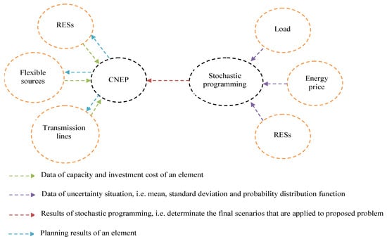
Figure 1.
The outline of the proposed stochastic coordinated network expansion planning (CNEP).
(A) Objective function: the objective function of the CNEP problem is expressed in Equation (1), and consists of five terms. The first one indicates the operation cost of generation units, and the second one presents the annual investment cost of the transmission expansion. The third and fourth terms refer to the RESs’ annual investment cost, and annual investment and operation cost of ESSs, respectively, and the flexibility index is formulated in the last term of the objective function. An annual step time in the horizon time is considered in this paper. Thus, the operation cost is multiplied by 8760, i.e., 24 × 365. It should be noted that the first and fifth terms of the objective function and the operation cost of ESS depend on uncertain parameters, while the second term, third term, and ESS investment costs do not. This means that the generating and ESS schedules are associated with the scenarios’ realization, as well as the system flexibility; however, the investment in new transmission lines, ESS, and RES cannot be changed by each scenario [32].
(B) AC power flow equations: These equations are introduced in (2)–(5), which correspond to the active and reactive power balance in each bus and time, (2) and (3), and the active and reactive power flow of lines in each time, (4) and (5), respectively. It should be noted that the multiplication of binary variable x in (4) and (5) is due to modeling the effect of the line construction. These constraints should be exerted only for the line candidates that are selected to be constructed. Also, note that the line between buses and is the same as the one between buses and . This fact is modeled by (6). In addition, A is a binary matrix whose elements represent the existence of transmission lines between different busses [21].
(C) System operation limitations: The operational limits of the system, i.e., the line capacity, the generating unit capacity, and the voltage limits, are expressed through (7)–(9) by the power flow equations [6].
(D) RES constraints: Constraint (10) presents the RES active power, where the maximum available power of RES (i.e., PRmax) is the function of wind speed/solar radiation for a wind/solar farm. Additionally, in constraint (10), if the RES i is constructed, = 1; otherwise, = 0.
(E) Flexibility resource constraints: The flexibility sources are ESSs in this paper due to their fast response characteristics [28], and hence, constraints (11)–(16) present the ESS operational equations. These constraints are charge rate limit, (11); discharge rate limit, (12); logical limit avoiding simultaneous ESS charging and discharging operation, (13); energy stored in an ESS, (14); minimum and maximum energy limits, (15); and the initial energy of an ESS, (16). Additionally, in constraints (13), (15), and (16), if the ESS i is constructed, = 1; otherwise, = 0.
(F) System flexibility constraints: This paper uses a metric to quantify the technical flexibility level of both individual flexible resources and the whole system based on the approach in [29]. This metric quantifies the technical ability of a system or resources to cope with the flexibility requirement resulting from the variability and the uncertainty produced by RESs. Flexible resources, i.e., ESSs, can be used to meet the system flexibility requirement. Also, there are upward and downward flexibility indices for each resource [29]. If the output power of flexible resources in the scenario ω is greater than its output power in the base case, there is upward flexibility for it. However, there is downward flexibility for the flexible resource if its output power in the scenario ω is less than the output power of this source in the base case [29]. The upward and downward flexibility for ESS can be obtained from (17). Moreover, system flexibility (SF) is calculated based on (18) [29].
2.2. The Linear CNEP Model
As can be observed from the aforementioned problem model, constraints (4), (5), (7) and (8) are nonlinear. In addition, Equations (4) and (5) are non-convex due to the terms of and [33,34,35], and they include a binary variable. Therefore, the model of (1)–(18) is a non-convex mixed-integer nonlinear problem (MINLP). This will slow down the solving procedure and may result in infeasible solutions in actual large-scale networks [36,37,38]. In this section, an equivalent linear model is proposed to speed up the solving procedure and guarantee the global optimality of the solution.
(A) The Linear approximation of AC power flow constraints: Nonlinear constraints in this section are (4) and (5). For linearizing these equations, the following assumptions are considered [38,39]:
- The difference in the voltage phases of the two ends of a transmission line is under 6 degrees or 0.105 radians.
- Since the magnitude of bus voltages in the transmission network should be between 0.95 and 1.05 per unit, the magnitude of bus voltages is very close to 1 per unit.
According to the mentioned assumptions, the bus voltages can be expressed as 1 + ΔV where the value of ΔV is much smaller than 1. Also, based on the first assumption, and are equal to 1 and , respectively. It is worth noting that the values of ΔV2, and are small enough to ignore, which is the case in this paper. Hence, Equations (4) and (5) are rewritten as below.
In order to linearize the multiplication of with other continuous terms, the big-M method can be used here as follows:
where M is a large enough number which is assumed to be 106. Also, the linearization procedure of Equation (23) is described in the next section.
(B) The linear approximation of system operation limitations: Equations (7), (8) and (23) are nonlinear. These relations represent circular inequalities, which denote the variation interval of active and reactive power inside a circle with a radius equal to the maximum apparent power. Nonetheless, determination of the linear equations corresponding to the circular plane with Equation (24) can be performed as illustrated in Figure 2 [36,37,38]. Hence, the circular plane is obtained by unifying several square planes. For example, based on Figure 2, the linear description of the circular plane is as in Equation (25).
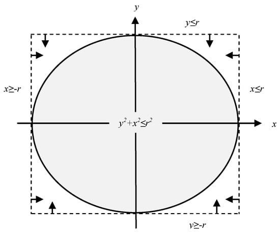
Figure 2.
The linearization of the circular plane.
According to Figure 2, Equation (24) has a large linearization error. Thereby, to reduce the linearization error, the number of square planes with different angles from the horizontal axis should be increased. Thus, at first 360 degrees of circle perimeter are divided into equal parts Δα. Then, the line equation is linearized for each k × Δα, where k is the counter of the linearized part. Finally, the calculated line equation is integrated with a circle with a radius less than or equal to r. Therefore, the linear approximation of the circular plane is expressed as below:
where nk denotes the number of linearized parts. For example, if 180 square planes are used for the linearization of a circular plane, nk and Δα will be equal to 180 and 2, respectively. Consequently, the planes x ≤ r and y ≤ r correspond to k = 0 and k = 45. Therefore, the linear approximation of (23) and (8) is as follows.
Therefore, the model of the mixed-integer linear problem (MILP) is proposed as:
Subject to:
(2), (3), (6), (10)–(18), (21), (22), (27) and (28)
As a final remark, in order to transform the model in (29)–(31) into a CNEP problem with DC power flow equations, the terms Q, ΔV, and g should be set to zero, and Equations (3), (22) and (31) must be removed. The term should be deleted from equations.
2.3. Uncertainties Model
In the proposed problem, the load parameters, i.e., PD and QD, the charging price (λ), and the maximum RES active power (PRmax) are considered to be the sources of uncertainty. In this paper, the roulette wheel mechanism (RWM) [27] for the generation of scenario samples is used for this case. It is noted that the RWM generates scenarios for load and price forecasting errors based on the normal distribution function [39], for the maximum RES active power based on Weibull distribution functions [27]. The Kantorovich method [27] is selected in this paper to reduce the number of scenarios, where the proposed scenario generation/reduction algorithm details are presented in [27].
3. Numerical Results and Discussion
To show the effectiveness of the proposed CNEP problem with AC power flow equations, it is tested on the IEEE 6-bus and IEEE 24-bus test systems, which are usually considered as test cases in previous research works in this area, such as [40,41,42]. Additionally, the proposed method is implemented in the GAMS software package using the solver of CPLEX/BONMIN for the MILP/MINLP problem [43]. An explanation about these solvers can be found in [44,45,46]. Note that the total number of linearization segments of circular constraint is considered to be 180 to obtain a low calculation error.
3.1. IEEE 6-Bus Test System
The diagram of the IEEE 6-bus test system is shown in Figure 3 [47], where bold lines denote the existing lines, and dashed lines represent the proposed lines to be constructed in the network. The power demand at the peak load hour, line data, and generator characteristics are described in Table 1, Table 2 and Table 3. Also, a planning horizon of 5 years is considered for the transmission lines. Table 4 represents the load percentage for each year, and the coincidence factor is considered to be 0.7 [21]. Moreover, it is forecasted that the wind farm with a capacity of 50 MW, and ESS with 200 MWh and charging/discharging rate of 50 MW and 88% efficiency can be installed in bus 4. Additionally, the forecasted daily load factor, the energy price, and the maximum RES (wind farm) power percentage are plotted in Figure 4 [34,48].
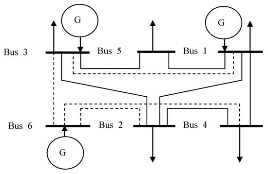
Figure 3.
Structure of 6-bus network [47].

Table 1.
Load characteristics of 6-bus network [47].
Table 2.
Line characteristics of 6-bus network [47].
Table 3.
Generator characteristics of 6-bus network [47].
Table 4.
Load percentage in different years.
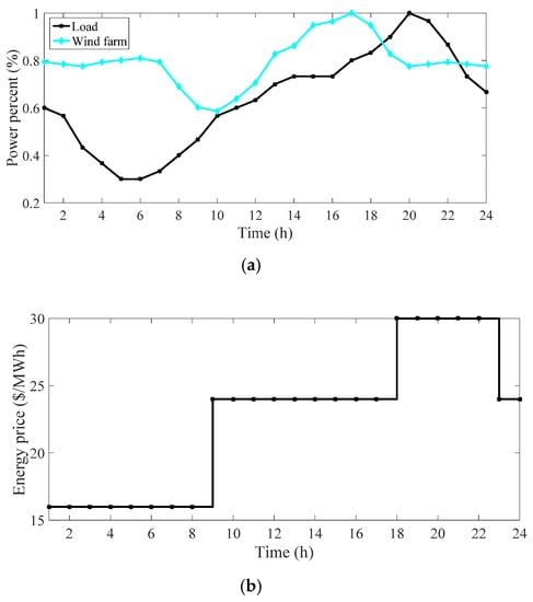
Figure 4.
(a) Daily curve of power percentage for the load [21] and wind farm [48], (b) energy price [34].
The base power and base voltage are equal to 100 MW and 230 kV, and the minimum and maximum voltage is 0.95 and 1.05 pu. Moreover, the reference bus is bus 1 with a voltage of 1.05∠0 pu.
(A) TEP Analysis: To compare the results and to understand better, for each test system, three different models have been tested as follows:
- Modeling of the TEP problem based on DC power flow equations (DCTEP) as an MILP problem.
- Modeling of the TEP problem based on nonlinear AC power flow equations (NACTEP) as an MINLP problem.
- Modeling of the TEP problem based on the linear approximation of AC power flow equations (LACTEP) as an MILP problem.
In this section, the deterministic TEP model considers only peak load hours, and both ESS and RES are removed from the proposed problem. The corresponding results for the three models are presented in Figure 5 and Table 5.
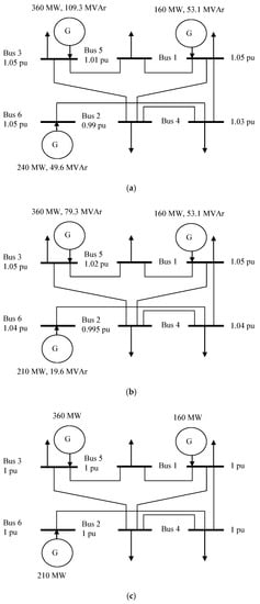
Figure 5.
Structure of 6-bus network that resulted from applying the proposed problem in the last year by using (a) NACTEP, (b) LACTEP, and (c) DCTEP.
Table 5.
Results of different factors in 6-bus network for different power flow methods.
According to this figure, the results of modeling of the TEP problem based on the DC power flow, the nonlinear power flow, and the linear approximation of AC power flow are the same in selecting the transmission lines for construction. For each of the three models, a transmission line is constructed between busses 4 and 6 by considering the load increase. However, it is seen that in Figure 5, the active and reactive power of generators and bus voltages have different values for different TEP models. The difference in bus voltages is negligible where linear or nonlinear AC power flow is used, but the difference in generators’ active and reactive power is about 3%. Also, it is observed that in the model based on DC power flow, bus voltages are always equal to 1 per unit and the reactive power is always zero.
Table 5 represents the obtained results for the operation and investment cost, constructed lines, network active and reactive losses, computation time, and the situation of problem-solving for three models. Based on this table, the construction cost is equal for the three models, due to their unique configuration. The exploitation cost and network’s active and reactive losses during the planning are equal in DC and linear AC power flow (models 1 and 3). Based on the obtained results, network losses in these two models are zero, due to the equations that are used in them. Since modeling based on nonlinear AC power flow (model 2) considers network losses, the operation cost of this model is greater than the two other ones. However, it is worth noting that model 2 as an MINLP problem achieves more accurate results, but its computation time is significantly larger than the computation time of models 1 and 3. Based on Table 6, model 2 does not have a globally optimal solution. Noticeably, the proposed TEP problem using linear AC power flow equations (model 3) possesses a slight approximation in comparison with model 2. It has a very small computation time and achieves a globally optimal solution. Also, the computation time of model 1 is short and it obtains an optimal solution, but the obtained result of this model is not feasible because the reactive power is not considered in DC power flow equations.
Table 6.
Results of different factors in 6-bus network for LACPF.
Herein, the results of the stochastic TEP method with the standard deviation of 10% for active and reactive load uncertainty are shown in Figure 6 and Table 6. By comparing Figure 5b and Figure 6, it is observed that in the stochastic model, two transmission lines are proposed to be constructed which include 2–6 and 4–6. Also, the expected active and reactive power of generators has been increased in comparison with the deterministic model, and the expected load bus voltages have been reduced. Based on Table 6, the total cost of operation and construction is about 153.368 M$, which will be equal to 93.062 M$ in the deterministic problem. The cost difference is 60.306 M$, which can be considered the prediction cost or the uncertainty cost or the security cost due to considering the load uncertainty.
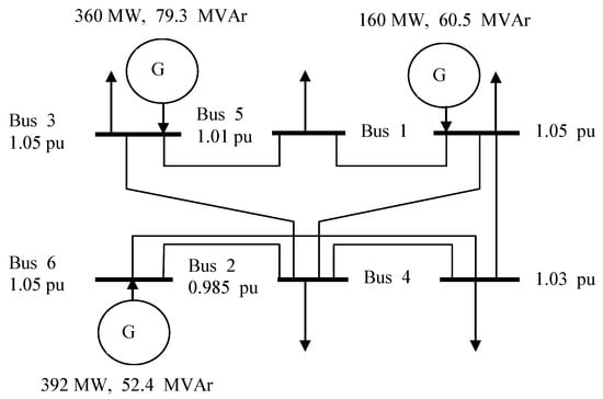
Figure 6.
Structure of 6-bus network that resulted from applying the proposed problem in the last year.
(B) CNEP capability: In this section, three cases are implemented on a 6-bus network to study the proposed stochastic CNEP problem as follows:
- Case I: The stochastic TEP method based on the linear AC power flow.
- Case II: The stochastic linear AC power flow-based CNEP (LAC-CNEP) method, considering renewable sources and the planning of transmission lines.
- Case III: The proposed stochastic LAC-CNEP method that is formulated in (29)–(31).
In this paper, the term FC is considered 2000 $ to obtain high flexibility in a 6-bus network. The results of three cases are presented in Table 7, and accordingly, it is seen that the proposed CNEP strategy has the following results:
Table 7.
The results of different methods of the proposed CNEP strategy.
- Reduce the operation cost: The operation cost in case II is 3,045,670 $, a reduction of 9.57% with respect to the TEP model. This term is 13.13% for the coordinated renewable sources and transmission expansion planning method.
- Reduce the investment cost: In the proposed CNEP method (case III), there is one constructed line that is between busses 2 and 6, while the TEP model includes two constructed lines.
- Improve the voltage profile: In case III, the maximum voltage drop is 0.053 p.u., while it is 0.065 and 0.059 p.u. in cases I and II, respectively. Therefore, the CNEP strategy can improve the voltage profile by about 18.46%.
- Obtain high flexibility: Based on Table 7, the CNEP method includes system flexibility of 10.93 as well as 0.2186 million $ flexibility benefit, where it is high concerning cases I and II.
3.2. IEEE 24-Bus Network
The 24-bus test system structure is presented in [14]. This network has 34 transmission lines, 24 of which exist, and 10 others of which are proposed for construction. The proposed lines for construction are shown in Table 8. Moreover, the wind farms with a capacity of 150 MW and ESSs with the maximum capacity of 400 MWh, 100 MW charging/discharging rate, and 88% efficiency can be connected to busses 13, 17, 21, and 23. The other data such as load factor, energy price, maximum RES power, etc., are the same as 6-bus test network data. The base power and base voltage of this network are 100 MVA and 230 kV, respectively.
Table 8.
The proposed line characteristics for construction.
The results for the proposed CNEP method are shown in Figure 7 and Figure 8. Figure 7 shows the energy profile of ESSs, in which the charging/discharging operation mode is represented by increasing/decreasing ESS energy. Accordingly, it is charged at the period of 1:00 to 8:00 due to the low energy price, and it is discharged at the period of 17:00 to 22:00 due to the high energy price as shown in Figure 4b. In other words, ESSs are charged during the low energy price period and are discharged at the high energy price time to have a low operation cost, based on objective function (1). Moreover, Figure 8 expresses the expected flexibility benefit and expected operation cost for the IEEE 24-bus network. According to Figure 8a, the expected flexibility benefit is increased by increasing the flexibility price (FC) to 105 $, and it is constant to 2.5 × 10⁵ if FC changes between 105 and 106 $. Also, the expected operation cost will be increased if FC increases between 0 and 105 $, and it is constant to 60 M$ if FC changes between 105 and 106 $. It is noted that the increase in FC causes the number of flexible sources or ESSs to be increased in the power system to obtain the high flexibility benefit; hence, the operation cost will be increased because a high number of ESSs is used in the power system in this condition. As a result, the CNEP can provide a transmission network with a lot of flexibility by setting a high flexibility incentive price. A suitable cost of operation value is also required. Finally, Table 9 presents the values of maximum voltage drop, system flexibility, and problem convergence. Accordingly, the maximum voltage drop from 1.05 p.u. is 0.064 p.u., which is less than the allowed value, i.e., 0.1 (1.05–0.95) p.u. Also, system flexibility is 19.4. In the end, these capabilities are calculated in 21 s, where the solution situation is optimal. Thus, the proposed method can obtain a reliable optimal solution in a low calculation time.
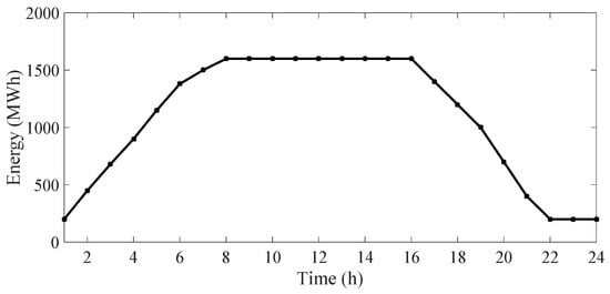
Figure 7.
Energy profile of energy storage systems (ESSs).
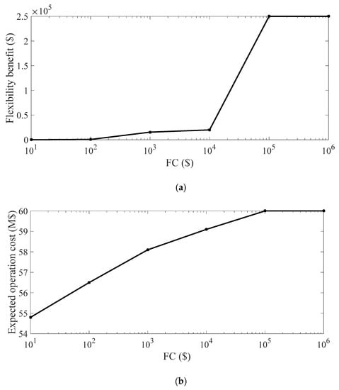
Figure 8.
(a) Flexibility benefit, (b) operation cost in FC.
Table 9.
Convergence, operation, and flexibility results.
4. Conclusions
This paper presents a method for the CNEP problem that minimizes the difference between investment and operation costs and flexibility benefit according to optimal power flow equations and planning constraints of different equipment. At first, the linear formulation of the AC optimal power flow model is used in the proposed strategy. Stochastic programming according to RWM-based scenario generation and Kantorovich method-based scenario reduction is used in this paper to model the forecasted error uncertainty of the load, energy price, and RES. Numerical results show that the proposed configuration structure by using MINLP and MILP models with linear AC and DC power flows is the same. The difference between the three models is in the network parameters, such as bus voltages and losses, the produced active and reactive power, and the operation cost. This difference is caused by the zero loss in MILP with AC power flow, and also the zero loss and reactive power and the 1 p.u. voltage in the MILP model with DC power flow. The difference in the first model is lower than in the second one. Also, two of the models have very short computation time and optimal solutions, while the MINLP model has a very long computation time and its solution is not an optimal one. The mentioned items indicate the superior performance of the MILP model by using linear AC power flow compared with the two other models. Thereby, the proposed CNEP strategy can improve the network indices such as the voltage profile, and it can allow high flexibility in the test system.
Author Contributions
M.R.A., conceptualization; S.P., validation and writing—original draft; M.K., methodology; A.N., edit and writing—original draft; M.B., supervision, analysis and interpretation of data. All authors have read and agreed to the published version of the manuscript.
Funding
The authors gratefully acknowledge financial support from the Universiti Teknologi Malaysia (Post-Doctoral Fellowship Scheme grant 05E09, and RUG grants 01M44, 02M18, 05G88, and 4B482).
Institutional Review Board Statement
Not applicable.
Informed Consent Statement
Not applicable.
Data Availability Statement
Data sharing not applicable. No new data were created or analyzed in this study.
Conflicts of Interest
The authors declare no conflict of interest.
Nomenclature
(1) Variables: All variables are in per unit (p.u.).
| ch, dch | Binary variable of charging and discharging state inflexible source (without unit) |
| E | Stored energy in the flexible source |
| F+, F− | Upward and downward flexibility active power |
| PFch, PFdch | Charging and discharging active power of flexible source |
| PG, QG | Active and reactive power of generation unit |
| PL, QL | Active and reactive power flow of line |
| PR | Active power of RES |
| SF | System flexibility (without unit) |
| V, ΔV, θ | Magnitude, deviation, and angle (in radian) of voltage |
| x, xR, xF | The binary variable of line, RES, and flexible source construction (without unit) |
(2) Constants:
| A | Bus incidence matrix (if a line existed between buses i and j, Ab,j is equal to 1, or otherwise zero) |
| C | Energy or operation price in $/MWh |
| CF | Coincidence factor |
| Eini | Initial energy of flexible source in p.u. |
| Emin, Emax | Minimum and maximum energy of flexible source in p.u. |
| FC | Flexibility price ($) |
| g, b | Conductance and susceptance of a line in p.u. |
| ICL, ICR, ICF | Investment cost of line, RES, and flexible source in $ |
| PD, QD | Active and reactive load in p.u. |
| PFmax | Maximum charge/discharge rate in p.u. |
| PRmax | Maximum RES active power in p.u. |
| Vmin, Vmax | Minimum and maximum value of voltage magnitude in p.u. |
| SLmax | Maximum capacity of line in p.u. |
| SGmax | Maximum capacity of generation unit in p.u. |
| ρ | Probability of scenario |
| λ | Energy price ($/MWh) |
| ηch, ηdch | Charging and discharging efficiency of flexible source |
(3) Sets and indices:
| (i, j), t, y, ω, k | Indices of bus, time, year, scenario, linearization segments of circular constraint |
| ϕi, ϕt, ϕy, ϕω, ϕk | Sets of bus, time, year, scenario, linearization segments of circular constraint |
References
- Jahannoosh, M.; Nowdeh, S.A.; Naderipour, A.; Kamyab, H.; Davoodkhani, I.F.; Klemeš, J.J. New Hybrid Meta-Heuristic Algorithm for Reliable and Cost-Effective Designing of Photovoltaic/Wind/Fuel Cell Energy System Considering Load Interruption Probability. J. Clean. Prod. 2020, 278, 123406. [Google Scholar] [CrossRef]
- Naderipour, A.; Abdul-Malek, Z.; Miveh, M.R.; Moghaddam, M.J.H.; Kalam, A.; Gandoman, F.H. A harmonic compensation strategy in a grid-connected photovoltaic system using zero-sequence control. Energies 2018, 11, 2629. [Google Scholar] [CrossRef]
- Naderipour, A.; Kalam, A.; Abdul-Malek, Z.; Davoudkhani, I.F.; Bin Mustafa, M.W.; Guerrero, J.M. An Effective Algorithm for MAED Problems with a New Reliability Model at the Microgrid. Electronics 2021, 10, 257. [Google Scholar] [CrossRef]
- Arabi-Nowdeh, S.; Nasri, S.; Saftjani, P.B.; Naderipour, A.; Abdul-Malek, Z.; Kamyab, H.; Nowdeh, A.J. Multi-criteria optimal design of hybrid clean energy system with battery storage considering off- and on-grid application. J. Clean. Prod. 2021, 290, 125808. [Google Scholar] [CrossRef]
- Fu, C.; Zhang, S.; Chao, K.-H. Energy Management of a Power System for Economic Load Dispatch Using the Artificial Intelligent Algorithm. Electronics 2020, 9, 108. [Google Scholar] [CrossRef]
- Bozorgavari, S.A.; Aghaei, J.; Pirouzi, S.; Vahidinasab, V.; Farahmand, H.; Korpås, M. Two-stage hybrid stochastic/robust optimal coordination of distributed battery storage planning and flexible energy management in smart distribution network. J. Energy Storage 2019, 26, 100970. [Google Scholar] [CrossRef]
- Alizadeh, B.; Jadid, S. Reliability constrained coordination of generation and transmission expansion planning in power systems using mixed integer programming. IET Gener. Transm. Distrib. 2011, 5, 948–960. [Google Scholar] [CrossRef]
- Jenabi, M.; Ghomi, S.F.; Smeers, Y. Bi-Level Game Approaches for Coordination of Generation and Transmission Expansion Planning Within a Market Environment. IEEE Trans. Power Syst. 2013, 28, 2639–2650. [Google Scholar] [CrossRef]
- Pozo, D.; Sauma, E.E.; Contreras, J. A three-level static MILP model for generation and transmission expansion planning. IEEE Trans. Power Syst. 2013, 28, 202–210. [Google Scholar] [CrossRef]
- Zhang, H.; Heydt, G.T.; Vittal, V.; Mittelmann, H.D. Transmission expansion planning using an ac model: Formulations and possible relaxations. In Proceedings of the 2012 IEEE Power and Energy Society General Meeting, San Diego, CA, USA, 22–26 July 2012; pp. 1–8. [Google Scholar] [CrossRef]
- Zhang, H.; Vittal, V.; Heydt, G.T.; Quintero, J. A Mixed-Integer Linear Programming Approach for Multi-Stage Security-Constrained Transmission Expansion Planning. IEEE Trans. Power Syst. 2011, 27, 1125–1133. [Google Scholar] [CrossRef]
- Santiago, P.T.; Carlos, A.C. Expansion planning for smart transmission grids using AC model and shunt compensation. IET Gener. Transm. Distrib. 2014, 8, 966–975. [Google Scholar]
- Alhamrouni, I.; Khairuddin, A.; Ferdavani, A.K.; Salem, M. Transmission expansion planning using AC-based differential evolution algorithm. IET Gener. Transm. Distrib. 2014, 8, 1637–1644. [Google Scholar] [CrossRef]
- Aghaei, J.; Amjady, N.; Baharvandi, A.; Akbari, M.-A. Generation and Transmission Expansion Planning: MILP–Based Probabilistic Model. IEEE Trans. Power Syst. 2014, 29, 1592–1601. [Google Scholar] [CrossRef]
- Mavalizadeh, H.; Ahmadi, A.; Heidari, A. Probabilistic multi-objective generation and transmission expansion planning problem using normal boundary intersection. IET Gener. Transm. Distrib. 2015, 9, 560–570. [Google Scholar] [CrossRef]
- Chen, B.; Wang, J.; Wang, L.; He, Y.; Wang, Z. Robust Optimization for Transmission Expansion Planning: Minimax Cost vs. Minimax Regret. IEEE Trans. Power Syst. 2014, 29, 3069–3077. [Google Scholar] [CrossRef]
- Moreira, A.; Pozo, D.; Street, A.; Sauma, E. Reliable renewable generation and transmission expansion planning: Co-optimization system’s resources for meeting renewable targets. IEEE Trans. Power Syst. 2017, 32, 3246–3257. [Google Scholar] [CrossRef]
- Hong, S.; Cheng, H.; Zeng, P. N-K Constrained Composite Generation and Transmission Expansion Planning With Interval Load. IEEE Access 2017, 5, 2779–2789. [Google Scholar] [CrossRef]
- Ahmadi, A.; Mavalizadeh, H.; Zobaa, A.F.; Shayanfar, H.A. Reliability-based model for generation and transmission expansion planning. IET Gener. Transm. Distrib. 2017, 11, 504–511. [Google Scholar] [CrossRef]
- Saxena, K.; Bhakar, R. Impact of LRIC pricing and demand response on generation and transmission expansion planning. IET Gener. Transm. Distrib. 2019, 13, 679–685. [Google Scholar] [CrossRef]
- Hamidpour, H.; Aghaei, J.; Dehghan, S.; Pirouzi, S.; Niknam, T. Integrated resource expansion planning of wind integrated power systems considering demand response programmes. IET Renew. Power Gener. 2019, 13, 519–529. [Google Scholar] [CrossRef]
- Najjar, M.; Falaghi, H. Wind-integrated simultaneous generation and transmission expansion planning considering short-circuit level constraint. IET Gener. Transm. Distrib. 2019, 13, 2808–2818. [Google Scholar] [CrossRef]
- Roldán, C.; Mínguez, R.; García-Bertrand, R.; Arroyo, J.M. Robust Transmission Network Expansion Planning under Correlated Uncertainty. IEEE Trans. Power Syst. 2019, 34, 2071–2082. [Google Scholar] [CrossRef]
- Huang, S.; Dinavahi, V. A Branch-and-Cut Benders Decomposition Algorithm for Transmission Expansion Planning. IEEE Syst. J. 2017, 13, 659–669. [Google Scholar] [CrossRef]
- Motie, S.; Keynia, F.; Ranjbar, M.R.; Maleki, A. Generation expansion planning by considering energy-efficiency programs in a competitive environment. Int. J. Electr. Power Energy Syst. 2016, 80, 109–118. [Google Scholar] [CrossRef]
- Nemati, H.; Latify, M.A.; Yousefi, G.R. Tri-level transmission expansion planning under intentional attacks: Virtual attacker approach—Part I: Formulation. IET Gener. Transm. Distrib. 2019, 13, 390–398. [Google Scholar] [CrossRef]
- Aghaei, J.; Barani, M.; Shafie-khah, M.; Sanchez de la Nieta, A.A.; Catalão, J.P.S. Risk-constrained offering strategy for aggregated hybrid power plant including wind power producer and demand response provider. IEEE Trans. Sustain. Energy 2016, 7, 513–525. [Google Scholar] [CrossRef]
- Zhang, Y.; Dong, Z.Y.; Luo, F.; Zheng, Y.; Meng, K.; Wong, K.P. Optimal allocation of battery energy storage systems in distribution networks with high wind power penetration. IET Renew. Power Gener. 2016, 10, 1105–1113. [Google Scholar] [CrossRef]
- Helistö, N.; Kiviluoma, J.; Holttinen, H. Long-term impact of variable generation and demand side flexibility on thermal power generation. IET Renew. Power Gener. 2018, 12, 718–726. [Google Scholar] [CrossRef]
- Zhang, W.; Maleki, A.; Rosen, M.A. A heuristic-based approach for optimizing a small independent solar and wind hybrid power scheme incorporating load forecasting. J. Clean. Prod. 2019, 241, 117920. [Google Scholar] [CrossRef]
- Maleki, A. Modeling and optimum design of an off-grid PV/WT/FC/diesel hybrid system considering different fuel prices. Int. J. Low Carbon Technol. 2018, 13, 140–147. [Google Scholar] [CrossRef]
- Conejo, A.J.; Baringo, L.; Kazempour, S.J.; Siddiqui, A.S. Investment in Electricity Generation and Transmission; Springer: Cham, Switzerland, 2016. [Google Scholar]
- Pirouzi, S.; Aghaei, J. Mathematical modeling of electric vehicles contributions in voltage security of smart distribution networks. Simulation 2018, 95, 429–439. [Google Scholar] [CrossRef]
- Pirouzi, S.; Aghaei, J.; Latify, M.A.; Yousefi, G.R.; Mokryani, G. A Robust Optimization Approach for Active and Reactive Power Management in Smart Distribution Networks Using Electric Vehicles. IEEE Syst. J. 2017, 12, 2699–2710. [Google Scholar] [CrossRef]
- Pirouzi, S.; Aghaei, J.; Shafie-khah, M.; Osório, G.J.; Catalão, J.P.S. Evaluating the security of electrical energy distribution networks in the presence of electric vehicles. In Proceedings of the IEEE PowerTech Conference, Manchester, UK, 18–22 June 2017; pp. 1–6. [Google Scholar]
- Pirouzi, S.; Aghaei, J.; Niknam, T.; Farahmand, H.; Korpås, M. Proactive operation of electric vehicles in harmonic polluted smart distribution networks. IET Gener. Transm. Distrib. 2018, 12, 967–975. [Google Scholar] [CrossRef]
- Pirouzi, S.; Aghaei, J.; Niknam, T.; Shafie-Khah, M.; Vahidinasab, V.; Catalão, J.P.S. Two alternative robust optimization models for flexible power management of electric vehicles in distribution networks. Energy 2017, 141, 635–652. [Google Scholar] [CrossRef]
- Pirouzi, S.; Aghaei, J.; Vahidinasab, V.; Niknam, T.; Khodaei, A. Robust linear architecture for active/reactive power scheduling of EV integrated smart distribution networks. Electr. Power Syst. Res. 2018, 155, 8–20. [Google Scholar] [CrossRef]
- Nikoobakht, A.; Mardaneh, M.; Aghaei, J.; Guerrero-Mestre, V.; Contreras, J. Flexible power system operation accommodating uncertain wind power generation using transmission topology control: An improved linearized AC SCUC model. IET Gener. Transm. Distrib. 2017, 11, 142–153. [Google Scholar] [CrossRef]
- Hagh, M.T.; Alipour, M.; Teimourzadeh, S. Application of HGSO to security based optimal placement and parameter setting of UPFC. Energy Convers. Manag. 2014, 86, 873–885. [Google Scholar] [CrossRef]
- Rabiee, A.; Shayanfar, H.A.; Amjady, N. Coupled energy and reactive power market clearing considering power system security. Energy Convers. Manag. 2009, 50, 907–915. [Google Scholar] [CrossRef]
- Esmaili, M.; Amjady, N.; Shayanfar, H.A. Stochastic congestion management in power markets using efficient scenario approaches. Energy Convers. Manag. 2010, 51, 2285–2293. [Google Scholar] [CrossRef]
- Generalized Algebraic Modeling Systems (GAMS). Available online: http://www.gams.com (accessed on 12 February 2021).
- Pirouzi, S.; Latify, M.A.; Yousefi, G.R. Conjugate active and reactive power management in a smart distribution network through electric vehicles: A mixed integer-linear programming model. Sustain. Energygrids Netw. 2020, 22, 100344. [Google Scholar] [CrossRef]
- Bozorgavari, S.A.; Aghaei, J.; Pirouzi, S.; Nikoobakht, A.; Farahmand, H.; Korpås, M. Robust planning of distributed battery energy storage systems in flexible smart distribution networks: A comprehensive study. Renew. Sustain. Energy Rev. 2020, 123, 109739. [Google Scholar] [CrossRef]
- Amjady, N.; Ansari, M.R. Non-convex security constrained optimal power flow by a new solution method composed of Benders decomposition and special ordered sets. Int. Trans. Electr. Energy Syst. 2014, 24, 842–857. [Google Scholar] [CrossRef]
- Rider, M.J.; Garcia, A.V.; Romero, R. Power system transmission network expansion planning using AC model. IET Gener. Transm. Distrib. 2007, 1, 731. [Google Scholar] [CrossRef]
- Maleki, A.; Askarzadeh, A. Optimal sizing of a PV/wind/diesel system with battery storage for electrification to an off-grid remote region: A case study of Rafsanjan, Iran. Sustain. Energy Technol. Assess. 2014, 7, 147–153. [Google Scholar] [CrossRef]


Publisher’s Note: MDPI stays neutral with regard to jurisdictional claims in published maps and institutional affiliations. |
© 2021 by the authors. Licensee MDPI, Basel, Switzerland. This article is an open access article distributed under the terms and conditions of the Creative Commons Attribution (CC BY) license (https://creativecommons.org/licenses/by/4.0/).