Application of Semi-Empirical Models Based on Satellite Images for Estimating Solar Irradiance in Korea

Abstract

The application of solar energy as a renewable energy source has significantly escalated owing to its abundance and availability worldwide. However, the intermittent behavior of solar irradiance is a serious disadvantage for electricity grids using photovoltaic (PV) systems. Thus, reliable solar irradiance data are vital to achieve consistent energy production. Geostationary satellite images have become a solution to this issue, as they represent a database for solar irradiance on a massive spatiotemporal scale. The estimation of global horizontal irradiance (GHI) using satellite images has been developed based on physical and semi-empirical models, but only a few studies have been dedicated to modeling GHI using semi-empirical models in Korea. Therefore, this study conducted a comparative analysis to determine the most suitable semi-empirical model of GHI in Korea. Considering their applicability, the Beyer, Rigollier, Hammer, and Perez, models were selected to estimate the GHI over Seoul, Korea. After a comparative evaluation, the Hammer model was determined to be the best model. This study also introduced a hybrid model and applied a long short-term memory (LSTM) model in order to improve prediction accuracy. The hybrid model exhibited a smaller root-mean-square error (RMSE), 97.08 W/m², than that of the Hammer model, 103.92 W/m², while producing a comparable mean-bias error. Meanwhile, the LSTM model showed the potential to further reduce the RMSE by 11.2%, compared to the hybrid model.

1. Introduction

Solar photovoltaic (PV) power has been widely utilized to cope with global warming and climate change, which are dominantly caused by the use of fossil fuels. Owing to its simple adaptation and low maintenance cost, solar PV technology is also becoming more common compared to other clean energies. However, the intermittent nature of solar irradiance is a major drawback that leads to unpredictable and uncontrollable electricity production from solar PV systems. Solar energy strongly depends on local meteorological factors, such as clouds and aerosol molecules, as well as sun position at a specific site. Therefore, solar irradiance data are critical for the optimization of solar PV power generation and the operation of solar PV systems [1,2,3,4].

The most reliable solar irradiance data are obtained from direct measurement using a pyranometer and pyrheliometer on the ground. Nowadays, the technology for irradiance measurement has advanced to the point that real-time data can be automatically collected and monitored. Nonetheless, ground measurement systems are expensive and require careful maintenance. As a result, ground measurement has limited spatial coverage, and the measurement database is still deficient for satisfying the demands of a PV-using society. Despite the attempts of some scholars to overcome the limited spatial coverage of direct measurement using conventional approaches, such as interpolation, the accuracy of the interpolated data is still not adequate [5,6].

Satellite data play an essential role in gathering information on solar irradiance on the earth’s surface. Zelenka et al. [5] showed that the accuracy of satellite-derived data is comparable with that of interpolated data from a station 25 km from the measurement site. The national solar radiation database in the United States has already taken advantage of satellite-driven irradiance data for nationwide coverage [7]. Geostationary satellites, whose orbit speed is identical to that of earth rotation, can repeatedly capture images of a specific area on the earth’s surface. The new generation of geostationary satellites are capable of delivering data images with a high spatial resolution of 1 × 1 km² for each visible channel image up to a 15-min time interval. Therefore, the solar irradiance data extracted from geostationary satellite images have a high potential for efficiently and inexpensively satisfying the demands of the solar energy sector.

Many researchers have developed and improved models to extract global horizontal irradiance (GHI) from satellite images [1,2,3,6,8,9,10,11,12]. The GHI estimation models are commonly in a physical or semi-empirical form. The physical models theoretically compute the extraterrestrial solar irradiance transmission through the atmosphere by calculating the radiative transfer equation. On the other hand, the semi-empirical models count on a linear interrelation between the satellite-recorded surface albedo and the clear-sky index, along with the consideration of important physical phenomena.

In terms of reliability and versatility, physical models have shown higher performance than semi-empirical models, as shown in

Table 1. Summary of semi-empirical and physical models using satellite images to estimate solar irradiance.

Reference	Year	Area	Köppen Climate Classification (Subtype)	Model	RMSE (W/m2)	rRMSE (%)	Satellite System
Beyer et al. [10]	1996	Germany	Continental (Dfb, Dfc) Temperate (Cfa, Cfb)	Semi-empirical	−	16	Meteosat-1
Perez et al. [2]	2002	United States	Dry (All subtypes) Temperate (All subtypes) Continental (All subtypes)	Semi-empirical	118	−	GOES
Hammer et al. [8]	2003	Europe	Dry (BSk, BWh) Temperate (Cfa, Cfb, Cfc, Csa, Csb) Continental (Dfa, Dfb)	Semi-empirical	−	35 (1 h ahead) 40 (2 h ahead)	Meteosat-2
Rigollier et al. [3]	2004	Europe	Dry (BSk, BWh) Temperate (Cfa, Cfb, Cfc, Csa, Csb) Continental (Dfa, Dfb)	Semi-empirical	− − −	45 (Jan 95) 27 (Apr 95) 18 (Jul 94)	Meteosat-1
Moradi et al. [11]	2009	Iran	Temperate (Csa)	Semi-empirical	−	11.7	Meteosat-5
Eissa et al. [12]	2012	United Arab Emirates	Dry (Bwh)	Semi-empirical	123	18.3	Meteosat-2
Choi et al. [15]	2015	Korea	Continental (Dwa)	Semi-empirical	−	30.8	COMS
Diallo et al. [6]	2018	French Guiana	Tropical (Af)	Semi-empirical	133	30	GOES
Yang et al. [4]	2020	Chengde	Continental (Dwa)	Semi-empirical	181 (1 h ahead) 200 (2 h ahead) 215 (3 h ahead)	−	Fengyun-4A
Jia et al. [16]	2021	Northern China	Continental (Dwa)	Semi-empirical	109	−	Fengyun-4A
Yeom et al. [17]	2012	Korea	Continental (Dwa)	Physical	71 (clear-sky) 90 (cloudy)	−	MTSAT-1R
Lefe’vre et al. [18]	2013	World	All classifications	Physical	35	7	Terra EOS
Zo et al. [19]	2014	Korea	Continental (Dwa)	Physical	85	−	COMS
Qu et al. [20]	2016	Europe and Africa	All classifications	Physical	90	18	Meteosat-2
Xie et al. [21]	2016	United States	Dry (All subtypes) Temperate (All subtypes) Continental (All subtypes)	Physical	130	−	−
Yeom et al. [22]	2016	Korea	Continental (Dwa)	Physical	72 (clear-sky) 106 (cloudy)	−	COMS
Kim et al. [23]	2016	Korea	Continental (Dwa)	Physical	65 (clear-sky) 149 (cloudy)	13 57	COMS

. However, physical models technically require more input of atmospheric data, such as aerosol optical depth (AOD), ozone content, and precipitable water. Such atmospheric data are often less accessible at a specific location than ground measurement data of solar irradiance. In contrast, semi-empirical models rely on simple assumptions and statistically determined coefficients. As a result, semi-empirical models require only a few input variables, and furthermore most of them are geometric factors. Semi-empirical models offer easier calculation, simpler implementation, and faster operation [13,14]. Due to their simplicity, semi-empirical models are often favorable for forecasting solar irradiance [8]. GHI forecasting means that the future values of input variables need to be known. The forecast accuracy of the physical model can quickly decrease with the number of input variables unless their values are properly forecast.

Cano et al. [9] proposed a pioneering form of the semi-empirical model, known as the Heliosat-1 model, which has become a fundamental technique for numerous following models. They assumed that the cloud index (CI) can be estimated based on the brightness of satellite sensor data. They calculated GHI by simply reducing clear-sky GHI according to the CI. Since then, Rigollier et al. [3], Perez et al. [2], Hammer et al. [8], Beyer et al. [10], and other scholars made improvements on the Cano model. As the well-known semi-empirical models were mainly developed using data in Europe and North America, many researchers evaluated and modified them for application to various other regions [6,11,12].

Table 1 implies that, based on Köppen–Geiger climate classification [24,25], the semi-empirical models were mostly dedicated to continental and temperate areas. Only a few studies addressed a hot summer continental climate, which is categorized as the “Dwa” subtype. In the northern region of China, Yang et al. [4] predicted GHI 1, 2, and 3 h ahead by using particle image velocimetry and the Rigollier method. Jia et al. [16] combined the McClear clear-sky irradiance [18] and Rigollier models to estimate GHI at Zhangbei. Both the studies utilized the Fengyun-4 satellite system.

In Korea, several studies have attempted to extract GHI from Korea’s Communication, Ocean, and Meteorological Satellite (COMS) system [15,17,19,22,23]. Since the COMS system was developed, most studies have focused on physical models. Zo et al. [19] initiated GHI modeling by using COMS data as input and introducing a physical model, which is called the Gangneung–Wonju National University (GWNU) model. Yeom et al. [22] applied the Kawamura model [26] and generated a solar irradiance map by considering topographical factors, such as terrain slope. In addition, Kim et al. [23] estimated GHI using their own physical model, which is called the CLAVR-x model. Still, as far as we know, only one such study has employed the semi-empirical method. Choi et al. [15] added a preprocessing algorithm into the Rigollier model to distinguish cloud from ground.

Considering the importance of semi-empirical models and the lack of relevant studies evaluating them in the hot summer continental climates, the present study focuses on two objectives. The first objective of this study is to conduct a comparative analysis of the existing semi-empirical solar irradiance models using data from Korea, and thus identify a semi-empirical model that is suitable for the hot summer continental climate. The second objective is to investigate the improvements in accuracy that could be achieved by combining formulas from various models and by applying a machine learning technique for replacing climate-dependent coefficients in the semi-empirical model. The fulfillment of these objectives will contribute to accurately estimating a regional database of solar radiation for the hot summer continental climate.

This paper consists of five sections. Section 2 presents ground station measurement of solar irradiance data, COMS satellite images, and AERONET data employed in this study. In Section 3, semi-empirical modeling methods, which include calculations of the cloud index, clear-sky irradiance, and GHI conversion, as well as the machine learning method, are explained. In addition, error metrics for accuracy evaluation of each model are listed. Detailed results, analyses, and discussions are presented in Section 4. Finally, Section 5 provides a summary of the major findings from the study.

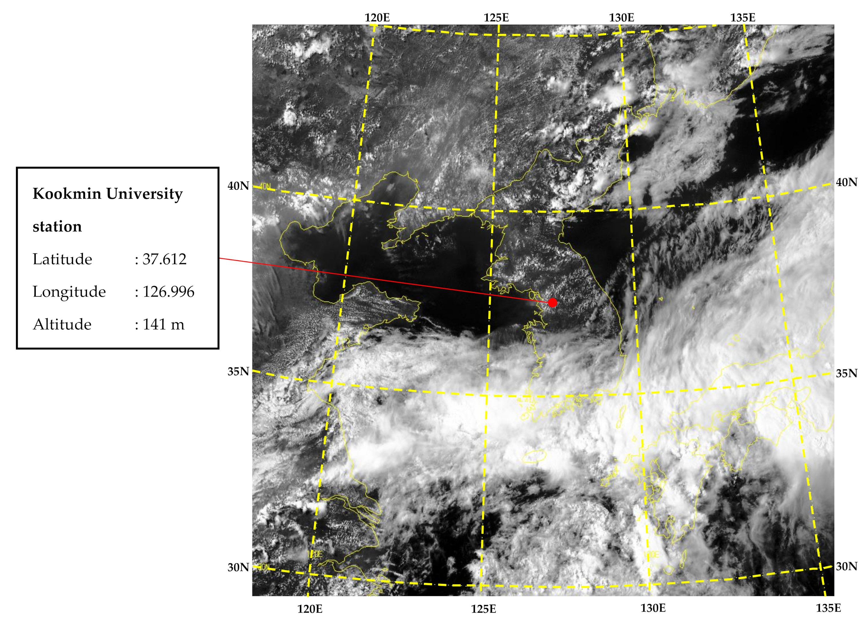
2. Satellite Images, Ground Measurement, and AERONET Dataset

The COMS has become a significant player in providing reliable weather data and atmospheric conditions since the Korean government launched its first geostationary satellite in 2011 at 128.2° E. The satellite system records the Korean peninsula and Asia-Pacific region, including the Australian continent, China, and Southeast Asia.

The COMS system carries three infrared (10.8 µm, 12 µm, and 3.7 µm), water vapor (6.7 µm), and visible (0.67 µm) channels to observe the earth’s surface. The images that COMS produced are composed of three levels of quality: level 1A, level 1B, and level 2. The level 1A images are satellite images processed through radiometric, geometric, and georeferencing calibration. In level 1B, images are then screened from distortion and nonuniform pixel intensity. Finally, images in level 2 are extracted into applicable maps, such as for forest fires, fog observation, and solar irradiance maps. Technically, the COMS satellite produces 16-bit visible images at 15-min intervals, and the satellite system provides a spatial resolution of 1 × 1 km² for the visible sensor and 4 × 4 km² for the three infrared channels. In this work, we utilized the hourly level 1B of satellite images (Figure 1) obtained from 1 January to 31 December 2018 and selected the pixel from each image that was closest to the ground measurement in order to validate our model.

This study performed GHI measurements from a ground station located in the northern part of Seoul (latitude, 37.612° N; longitude, 126.996° E; and altitude, 141 m). The ground measurement system comprises one pyranometer (MS-802 model) for the GHI and one pyrheliometer (MS-57 model) for direct normal irradiance (DNI). Both of the instruments, manufactured by the Eko company in Japan, have a sensitivity around ±7 µVm²/W for the GHI and DNI, respectively [27,28]. Identical to the COMS satellite data, hourly intervals for the ground data were also locally archived from 1 January–31 December 2018.

In this study, quality control was applied based on the procedure from Gueymard and Ruiz-Arias [29] to guarantee reliable data from the ground measurement. In particular, data that did not meet the following criteria were rejected:

• ${\mathsf{\theta }}_{\mathrm{z}}>{80}^{\circ }$
• $\mathrm{GHI}>0 \mathrm{W}/{\mathrm{m}}^2$
• $\mathrm{GHI}<1.5{\mathrm{G}}_{\mathrm{ext}}{\cos }^{1.2}{\mathsf{\theta }}_{\mathrm{z}}+100 \mathrm{W}/{\mathrm{m}}^2$
• $\mathrm{DNI}\ge 0 \mathrm{W}/{\mathrm{m}}^2$
• $\mathrm{DNI}\le G_{ext}$,

where ${\mathsf{\theta }}_{\mathrm{z}}$ and $G_{ext}$ denoted the solar zenith angle and extraterrestrial irradiance on a normal surface, respectively. The data that did not meet the requirements were rejected. Note that the criterion of ${\mathsf{\theta }}_{\mathrm{z}}>{80}^{\circ }$ was applied to remove GHI values at low sun elevation, and DNI data only were used for the data quality control.

The aerosol robotic network (AERONET) is a network of ground-based measurements providing continuous data on spectral AOD, precipitable water, and inversion aerosol in various aerosol regimes using a sun radiometer [30]. The sun–sky radiometer system of AERONET quantifies solar spectral measurements every 15 min through eight spectral bands at wavelengths of 340, 380, 440, 500, 675, 870, 940, and 1020 nm [31]. The AERONET dataset has three grades: level 1 for raw data, level 1.5 for data with clouds removed, and level 2 for quality-controlled data. In this study, clear-sky irradiance was calculated through the Linke turbidity factor ($T_L$) to consider the reduction of solar irradiance owing to atmospheric effects. The level 2 data of AERONET, which were collected from 1 January–31 December 2018, were employed and arranged into hourly intervals to determine the value of $T_L$.

3. Global Horizontal Irradiance Models

In this study, from their accuracy, applicability, and versatility, well-known semi-empirical models were chosen to generate the GHI over the Korea peninsula [1,3,8,11]. The Beyer, Rigollier, and Hammer models originally utilized the Meteosat imagery system and their results were validated through ground measurements located in Europe. Beyer et al. [10] modified the original Heliosat-1 model by introducing new variants for geometrical correction, backscatter correction, and clear-sky irradiance computation. It was revealed that the hourly insolation accuracy of the Beyer model has an RMSE of 120 Wh/m² (rRMSE of 16%). Rigollier et al. [3] improved the Heliosat-1 method by applying calibrated radiances instead of digital numbers. The application of the calibrated radiances as input opened the opportunity for substituting several empirical components of Heliosat-1 into the physical computation. The results of the Rigollier model revealed RMSEs and rRMSEs of 62 Wh/m² (45%), 96 Wh/m² (27%), and 103 Wh/m² (18%) for January 1995, April 1995, and July 1994, respectively.

The Hammer model was established to forecast the GHI several hours ahead. A motion vector field from two consecutive satellite images can be generated to determine cloud motion. The vector field was computed with the current images and extrapolated up to 120 min ahead with a 30-min interval. Finally, the GHI could be forecast by applying the extrapolated pixels of the satellite image to the Hammer model. The relative RMSEs (rRMSE) were 35% and 40% for 1-h and 2-h forecast horizons, respectively. Contrary to the other three models, the Perez model used the geostationary operational environmental satellite (GOES) system in the United States. Validation of the Perez model was then conducted against ten ground measurements from different climatic types of the American region. The RMSE of the Perez model varied from 44 to 118 W/m², depending on the location of the ground measurement. Below are the detailed explanations of the procedures used for each model.

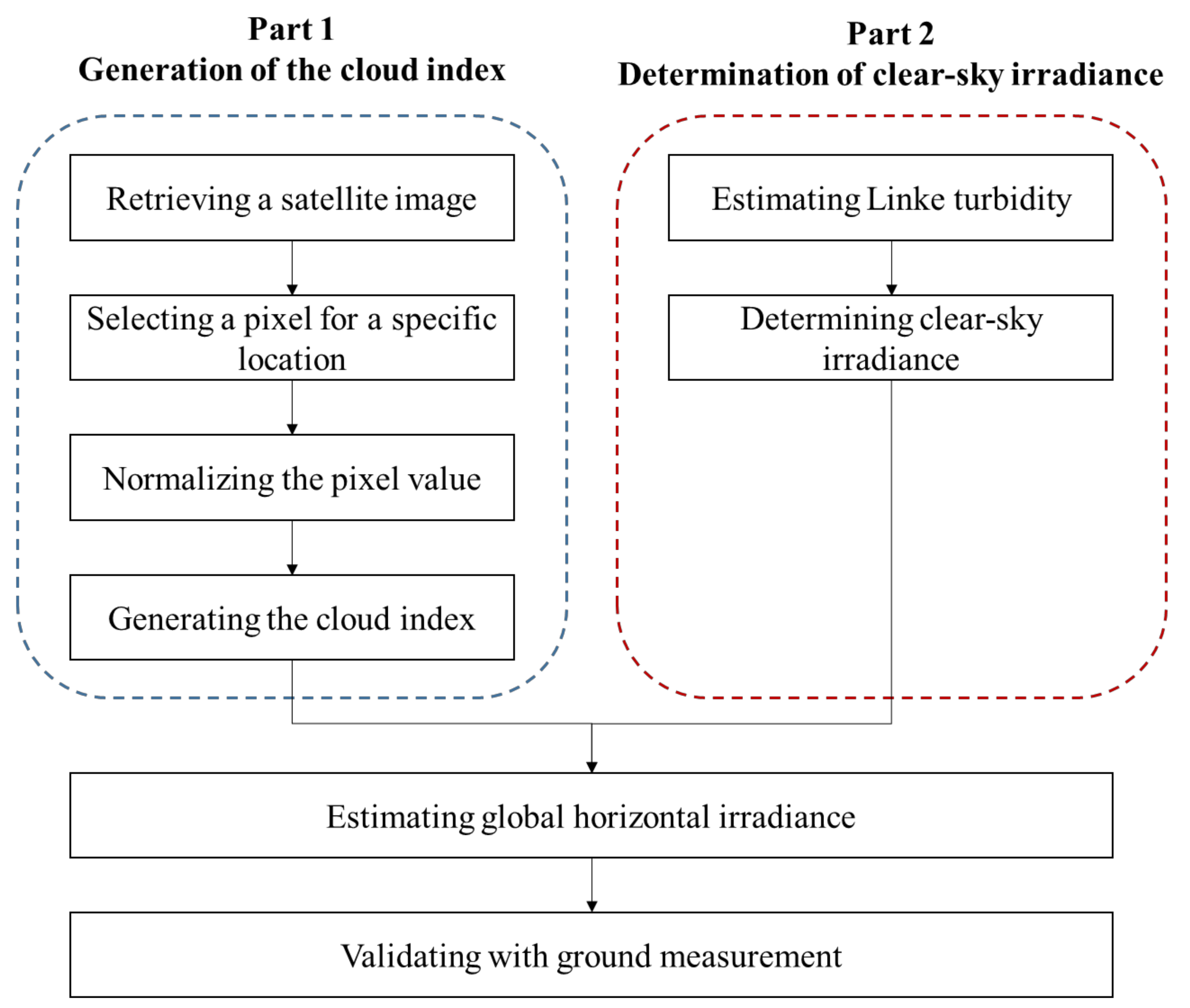
3.1. Cloud Index Formula

The schematic diagram in Figure 2 illustrates the flow to derive the GHI using the semi-empirical models. The two important procedures are the CI estimation, which represents the cloudiness over the earth’s surface based on a satellite image, and the calculation of the clear-sky irradiance using atmospheric data. Thus, the GHI can be determined as the decrease in the clear-sky irradiance due to the CI.

Normalization of satellite image data is mandatory to obtain a CI that is independent from optical and geometric effects [1]. The air mass and backscatter effects mainly cause optical distortion in image data. The air mass effect occurs because sunlight is scattered and absorbed by particles when it passes through the atmosphere. As a result, the closer the sun is to the horizon, the stronger the air mass effect is. The backscatter effect, which is also known as the hot-spot effect, implies that sunlight more significantly goes back in the sun’s direction after scattering by atmospheric particles. Thus, the sensor system overestimates the ground albedo when the satellite is close to the sun.

Each semi-empirical model has its own correction formula, which was originally developed using its satellite systems and local stations. The conversion formulas from raw satellite pixel data ($C_{sat}$) to normalized data ($CC$) are presented in Table 2. The Beyer and Hammer models include a correction factor ($C_0$) for the air mass and backscattering effects, where $C_0$ is determined through ${\mathsf{\theta }}_{\mathrm{z}}$, backscattering angle ($\mathsf{\psi }$), and satellite zenith angle ($\mathsf{\phi }$). The production of the solar constant ($I_0$) and the eccentricity correction of the sun-to-earth distance ($\mathsf{\epsilon }$) represent the extraterrestrial irradiance.

The Rigollier model extracted its correction factor ($C_{0R}$) using some equations from the European Solar Radiation Atlas (ESRA) model. To obtain $C{C}_R$, clear-sky diffuse irradiance (${\mathrm{DHI}}_{cR}$), transmittance from the sun to the earth ($T$), and transmittance from the earth to the satellite system ($T_{sat}$) were computed. The parameters ${\mathsf{\theta }}_{\mathrm{z}}$, $\mathsf{\phi }$, and $T_L$ were the key input variables for determining the energy that is scattered in the atmosphere and evaluated via the ESRA model. The maximum total irradiance of the visible sensor ($I_{0met}$) was obtained from the convolution of the spectral distribution of $I_0$ by the spectral sensitivity curve of the radiometer [3]. To obtain further details on the normalization process, the reader is encouraged to refer to Rigollier et al. [3] and the ESRA [32].

Contrary to the other three models, the Perez model introduced dependence on the sun elevation ($\mathsf{\gamma }$) and air mass ($AM$) to normalize pixels from air mass effect. Perez et al. [2] evaluated the backscatter correction by deriving different lower boundaries of the dynamic range from several years of recorded satellite data. However, the present study only used the data of a single year, and the backscatter effect was not considered.

In addition to the models chosen in this study, more models are available throughout the literature. The combination of formulas used by various models was attempted to investigate the possibility of increasing prediction accuracy. As a result, the normalization equations provided by Zelenka et al. [5], the clear-sky irradiance equation given by Kasten [33], and the GHI conversion equation proposed by Perez et al. [2] were combined to create a single model. In this study, this model will be referred to as the hybrid model. Originally, Zelenka et al. [5] used ${\mathsf{\theta }}_{\mathrm{z}}$ and $\mathsf{\psi }$ as the correction factor ($C_{0M}$) to normalize ground albedo ($C_{\min }$).

Clouds are the main factor attenuating solar irradiance when sunlight penetrates the atmospheric layer. The CI, which is used to represent the amount of clouds in the sky, can be estimated via a relative difference in the normalized pixel value between the lower and upper boundaries of its dynamic range. The lower and upper boundaries can be interpreted as the earth’s surface and cloud reflectance, respectively. Cloud index can be determined according to the previous studies [8,10,34]:

$$\mathrm{CI}=\frac{CC-C_{\min }}{C_{\max }-C_{\min }}$$

(1)

where $C_{\max }$ and $C_{\min }$ denote the highest and lowest values of $CC$, respectively. The CI value ranges from zero, which represents the darkest condition (no clouds) to unity, which represents the brightest condition (overcast). For the Rigollier model, $C_{\max }$ should be obtained in the same way as $C{C}_R$, but using the effective cloud albedo formulation, as follows [3]:

$$C_{\max R}=\frac{0.78-0.13[1-\exp (-4\cos {({\mathsf{\theta }}_{\mathrm{z}})}^5)]-C_{0R}}{T({\mathsf{\theta }}_{\mathrm{z}},T_L)T_{sat}(\mathsf{\phi },T_L)}$$

(2)

Table 2. Pixel normalization formulas for obtaining an independent cloud index (CI) (step 2). Each “raw” pixel ($C_{sat}$) is subjected to this normalization before CI extraction.

Model	Equation
Beyer	$C{C}_B=\frac{C_{sat}-C_{0B}}{(0.7)\mathsf{\epsilon }\cos {\mathsf{\theta }}_{\mathrm{z}}{\cos }^{0.15}{\mathsf{\theta }}_{\mathrm{z}}}$	(3)
	$C_{0B}=4.3+\left[4.5(1+{\cos }^2\mathsf{\psi })\frac{{\cos }^{0.15}{\mathsf{\theta }}_{\mathrm{z}}}{{\cos }^{0.8}\mathsf{\phi }}\right]$	(4)
Rigollier	$C{C}_R=\frac{C_{sat}-C_{0R}}{T({\mathsf{\theta }}_{\mathrm{z}},T_L)T_{sat}(\mathsf{\phi },T_L)}$	(5)
	$C_{0R}=\left(\frac{{\mathrm{DHI}}_{cR}}{\pi }\right)\left(\frac{I_{0\mathrm{m}et}}{I_0}\right){\left(\frac{0.5}{\cos \mathsf{\phi }}\right)}^{0.8}$	(6)
Hammer	$C{C}_H=\frac{C_{sat}-C_{0H}}{I_0\mathsf{\epsilon }\cos {\mathsf{\theta }}_{\mathrm{z}}}$	(7)
	$C_{0H}=4.3+\left[(1+{\cos }^2\mathsf{\psi })\frac{F_H}{{\cos }^{0.78}\mathsf{\phi }}\right]$	(8)
	$F_H=-0.55-25.2\cos {\mathsf{\theta }}_{\mathrm{z}}-38.3{\cos }^2{\mathsf{\theta }}_{\mathrm{z}}+17.7{\cos }^3{\mathsf{\theta }}_{\mathrm{z}}$	(9)
Perez	$C{C}_P=\frac{C_{sat}AM\mathsf{\epsilon }}{2.283{\mathsf{\gamma }}^{-0.26}\exp (0.004\mathsf{\gamma })}$	(10)
Hybrid	$C{C}_M=\frac{C_{sat}}{C_{0M}}$	(11)
	$C_{0M}=\left[0.85+0.15\left(\frac{\cos {\mathsf{\theta }}_{\mathrm{z}}+\sin {\mathsf{\theta }}_{\mathrm{z}}\exp (0.04-0.04AM)}{\cos {\mathsf{\theta }}_{\mathrm{z}}(\cos {\mathsf{\theta }}_{\mathrm{z}}+\sin {\mathsf{\theta }}_{\mathrm{z}})}\right)\right]\left[1+0.7{\left(\frac{50-\mathsf{\psi }}{50}\right)}^2\right]$	(12)

Table 2. Pixel normalization formulas for obtaining an independent cloud index (CI) (step 2). Each “raw” pixel ($C_{sat}$) is subjected to this normalization before CI extraction.

Model	Equation
Beyer	$C{C}_B=\frac{C_{sat}-C_{0B}}{(0.7)\mathsf{\epsilon }\cos {\mathsf{\theta }}_{\mathrm{z}}{\cos }^{0.15}{\mathsf{\theta }}_{\mathrm{z}}}$	(3)
	$C_{0B}=4.3+\left[4.5(1+{\cos }^2\mathsf{\psi })\frac{{\cos }^{0.15}{\mathsf{\theta }}_{\mathrm{z}}}{{\cos }^{0.8}\mathsf{\phi }}\right]$	(4)
Rigollier	$C{C}_R=\frac{C_{sat}-C_{0R}}{T({\mathsf{\theta }}_{\mathrm{z}},T_L)T_{sat}(\mathsf{\phi },T_L)}$	(5)
	$C_{0R}=\left(\frac{{\mathrm{DHI}}_{cR}}{\pi }\right)\left(\frac{I_{0\mathrm{m}et}}{I_0}\right){\left(\frac{0.5}{\cos \mathsf{\phi }}\right)}^{0.8}$	(6)
Hammer	$C{C}_H=\frac{C_{sat}-C_{0H}}{I_0\mathsf{\epsilon }\cos {\mathsf{\theta }}_{\mathrm{z}}}$	(7)
	$C_{0H}=4.3+\left[(1+{\cos }^2\mathsf{\psi })\frac{F_H}{{\cos }^{0.78}\mathsf{\phi }}\right]$	(8)
	$F_H=-0.55-25.2\cos {\mathsf{\theta }}_{\mathrm{z}}-38.3{\cos }^2{\mathsf{\theta }}_{\mathrm{z}}+17.7{\cos }^3{\mathsf{\theta }}_{\mathrm{z}}$	(9)
Perez	$C{C}_P=\frac{C_{sat}AM\mathsf{\epsilon }}{2.283{\mathsf{\gamma }}^{-0.26}\exp (0.004\mathsf{\gamma })}$	(10)
Hybrid	$C{C}_M=\frac{C_{sat}}{C_{0M}}$	(11)
	$C_{0M}=\left[0.85+0.15\left(\frac{\cos {\mathsf{\theta }}_{\mathrm{z}}+\sin {\mathsf{\theta }}_{\mathrm{z}}\exp (0.04-0.04AM)}{\cos {\mathsf{\theta }}_{\mathrm{z}}(\cos {\mathsf{\theta }}_{\mathrm{z}}+\sin {\mathsf{\theta }}_{\mathrm{z}})}\right)\right]\left[1+0.7{\left(\frac{50-\mathsf{\psi }}{50}\right)}^2\right]$	(12)

3.2. Clear-Sky Irradiance Formula

Another essential element of semi-empirical models is the determination of the maximum solar irradiance limit, i.e., the clear-sky irradiance (${\mathrm{GHI}}_c$). Under a cloudless condition, the solar irradiance attenuation depends on the concentration of absorbers and scatterers, such as aerosols, gases, and water vapor, inside the atmosphere. Most clear-sky models address solar attenuation through a derivation from atmospheric components and geometric position. With regard to the semi-empirical approach, the complexity of the clear-sky irradiance model, which is caused by rapid changes in aerosols, water vapor, and other molecules, is relatively reduced. The atmospheric variables can instead be simplified into a single turbidity variable of $T_L$ [35,36,37]. In this study, well-known clear-sky irradiance models (Table 3) were selected to examine ${\mathrm{GHI}}_c$.

The Beyer model applies a straightforward clear-sky model based on only a geometric calculation. This model is called the Bourges clear-sky formula and uses only ${\mathsf{\theta }}_{\mathrm{z}}$ to summarize the attenuation of extraterrestrial solar irradiance during transmission in the atmosphere [10]. The model was purely developed from an empirical correlation between ground measurement, sun position, and site location [38].

The clear-sky irradiance of the Rigollier model, which is known as the ESRA model, is decomposed into direct and diffuse components, considering $T_L$ and the Rayleigh scattering factor (${\delta }_R$). The clear-sky irradiance formula of the Hammer model is similar to that of the Rigollier model. The clear-sky DNI equations in both the Rigollier and Hammer models are identical [39], but the clear-sky DHI equations are different.

Owing to the complexities in the derivation of the clear-sky GHI from the Rigollier model, it was preferable to adopt a simpler formula, successfully applied in previous literature. Here, the Kasten clear-sky model was selected to determine the clear-sky GHI of the hybrid model. The model conserved site elevation ($\mathrm{z}$) and atmosphere turbidity for a site. By including $\mathrm{z}$ in the equation, the Kasten model demonstrated its advantage in investigating clear-sky GHI at high elevations. In the Perez model, the clear-sky GHI is calculated based on the study by Ineichen and Perez [36], in which they upgraded the original Kasten model. This new variant also considers $T_L$ and $\mathrm{z}$ to enhance its suitability for observational data from the West of the American continent.

The most important input parameter in the clear-sky model is the Linke turbidity, which accounts for atmospheric conditions. The Linke turbidity is also a convenient tool for simplifying the degree of atmospheric attenuation due to absorption and scattering. Theoretically, $T_L$ can be evaluated via either a direct or indirect formula [40]. The direct formula, which is called the pyrheliometric formula, commonly exploits DNI measurement data, $AM$, and ${\delta }_R$ [2]. In contrast, the indirect formula, which is called the parameterized formula, uses atmospheric components, such as $AM$, precipitable water vapor ($w$), angstrom turbidity factor ($\mathsf{\beta }$), and AOD [41]. After testing various formulas of $T_L$, the model introduced by Remund et al. [41] (Equation (13)) turned out to be optimal and was used throughout this study:

$$T_L=(1.8498+0.2425w-0.0203w^2)+(15.427+0.3153w-0.0254w^2)\mathsf{\beta }$$

(13)

Table 3. Clear-sky irradiance formulas used for each semi-empirical model.

Model	Equation
Beyer	${\mathrm{GHI}}_{cB}=0.7I_0\mathsf{\epsilon }{\cos }^{1.15}{\mathsf{\theta }}_{\mathrm{z}}$	(14)
Rigollier	${\mathrm{GHI}}_{cR}={\mathrm{DNI}}_{cR}\cos {\mathsf{\theta }}_{\mathrm{z}}+{\mathrm{DHI}}_{cR}$	(15)
	${\mathrm{DNI}}_{cR}=I_0\mathsf{\epsilon }\cos {\mathsf{\theta }}_{\mathrm{z}}\exp (-0.8662T_L{\mathsf{\delta }}_{R}AM)$	(16)
	${\mathrm{DHI}}_{cR}=I_0\mathsf{\epsilon }{T}_{rd}{F}_R$	(17)
	$T_{rd}=-0.015843+0.03543T_L+0.0003797T_L{}^2$	(18)
	$F_R=A_0+A_1\cos {\mathsf{\theta }}_{\mathrm{z}}+A_2{\cos }^2{\mathsf{\theta }}_{\mathrm{z}}$	(19)
	$A_0=0.26463-0.061581T_L+0.0031408T_L{}^2$	(20)
	$A_1=2.0402-0.018945T_L+0.01161T_L{}^2$	(21)
	$A_2=-1.3025-0.039231T_L+0.0085079T_L{}^2$	(22)
Hammer	${\mathrm{GHI}}_{cH}={\mathrm{DNI}}_{cH}\cos {\mathsf{\theta }}_{\mathrm{z}}+{\mathrm{DHI}}_{cH}$	(23)
	${\mathrm{DNI}}_{cH}=I_0{\mathsf{\epsilon }\cos \mathsf{\theta }}_{\mathrm{z}}\exp (-0.8662T_L{\mathsf{\delta }}_{R}AM)$	(24)
	${\mathrm{DHI}}_{cH}={\mathrm{G}}_{ext}\mathsf{\epsilon }\left[\begin{array}{l}0.0065+(-0.045+0.0646T_L)\cos {\mathsf{\theta }}_{\mathrm{z}}+\\ (0.014-0.0326T_L){\cos }^2{\mathsf{\theta }}_{\mathrm{z}}\end{array}\right]$	(25)
Perez	${\mathrm{GHI}}_{cP}=cg1I_0\cos {\mathsf{\theta }}_{\mathrm{z}}\exp [-cg2AM(fh1+fh2(T_L-1))]\exp (0.01A{M}^{1.8})$	(26)
	$fh1=\exp \left(\frac{-\mathrm{z}}{8000}\right)$	(27)
	$fh2=\exp \left(\frac{-\mathrm{z}}{1250}\right)$	(28)
	$cg1=0.0000509\mathrm{z}+0.868$	(29)
	$cg2=0.0000392\mathrm{z}+0.0387$	(30)
Hybrid	${\mathrm{GHI}}_{cM}=0.84I_0\cos {\mathsf{\theta }}_{\mathrm{z}}\exp [-0.027AM(fh1+(T_L-1)fh2)]$	(31)

Table 3. Clear-sky irradiance formulas used for each semi-empirical model.

Model	Equation
Beyer	${\mathrm{GHI}}_{cB}=0.7I_0\mathsf{\epsilon }{\cos }^{1.15}{\mathsf{\theta }}_{\mathrm{z}}$	(14)
Rigollier	${\mathrm{GHI}}_{cR}={\mathrm{DNI}}_{cR}\cos {\mathsf{\theta }}_{\mathrm{z}}+{\mathrm{DHI}}_{cR}$	(15)
	${\mathrm{DNI}}_{cR}=I_0\mathsf{\epsilon }\cos {\mathsf{\theta }}_{\mathrm{z}}\exp (-0.8662T_L{\mathsf{\delta }}_{R}AM)$	(16)
	${\mathrm{DHI}}_{cR}=I_0\mathsf{\epsilon }{T}_{rd}{F}_R$	(17)
	$T_{rd}=-0.015843+0.03543T_L+0.0003797T_L{}^2$	(18)
	$F_R=A_0+A_1\cos {\mathsf{\theta }}_{\mathrm{z}}+A_2{\cos }^2{\mathsf{\theta }}_{\mathrm{z}}$	(19)
	$A_0=0.26463-0.061581T_L+0.0031408T_L{}^2$	(20)
	$A_1=2.0402-0.018945T_L+0.01161T_L{}^2$	(21)
	$A_2=-1.3025-0.039231T_L+0.0085079T_L{}^2$	(22)
Hammer	${\mathrm{GHI}}_{cH}={\mathrm{DNI}}_{cH}\cos {\mathsf{\theta }}_{\mathrm{z}}+{\mathrm{DHI}}_{cH}$	(23)
	${\mathrm{DNI}}_{cH}=I_0{\mathsf{\epsilon }\cos \mathsf{\theta }}_{\mathrm{z}}\exp (-0.8662T_L{\mathsf{\delta }}_{R}AM)$	(24)
	${\mathrm{DHI}}_{cH}={\mathrm{G}}_{ext}\mathsf{\epsilon }\left[\begin{array}{l}0.0065+(-0.045+0.0646T_L)\cos {\mathsf{\theta }}_{\mathrm{z}}+\\ (0.014-0.0326T_L){\cos }^2{\mathsf{\theta }}_{\mathrm{z}}\end{array}\right]$	(25)
Perez	${\mathrm{GHI}}_{cP}=cg1I_0\cos {\mathsf{\theta }}_{\mathrm{z}}\exp [-cg2AM(fh1+fh2(T_L-1))]\exp (0.01A{M}^{1.8})$	(26)
	$fh1=\exp \left(\frac{-\mathrm{z}}{8000}\right)$	(27)
	$fh2=\exp \left(\frac{-\mathrm{z}}{1250}\right)$	(28)
	$cg1=0.0000509\mathrm{z}+0.868$	(29)
	$cg2=0.0000392\mathrm{z}+0.0387$	(30)
Hybrid	${\mathrm{GHI}}_{cM}=0.84I_0\cos {\mathsf{\theta }}_{\mathrm{z}}\exp [-0.027AM(fh1+(T_L-1)fh2)]$	(31)

3.3. GHI Conversion Formula

After CI and ${\mathrm{GHI}}_c$ are given, the GHI can be calculated from ${\mathrm{GHI}}_c$ by appropriately reducing it according to CI. The reduction factor is called the clear-sky index ($k_c$) and is expressed as a correlation function. Finally, the conversion equations are presented in

Table 4. Global horizontal irradiance (GHI) conversion used for each semi-empirical model.

Model	Equation
Beyer	${\mathrm{GHI}}_B=k_{cB}{\mathrm{GHI}}_{cB}$	(33)
	$k_{cB}=1-{\mathrm{CI}}_B$	(34)
Rigollier	${\mathrm{GHI}}_R=k_{cR}{\mathrm{GHI}}_{cR}$	(35)
	${\mathrm{CI}}_R\le -0.2;k_{cR}=1.2$	(36)
	$-0.2<{\mathrm{CI}}_R\le 0.8;k_{cR}=1-{\mathrm{CI}}_R$
	$0.8<{\mathrm{CI}}_R\le 1.1;k_{cR}=2.0667-3.6667{\mathrm{CI}}_R+1.6667{\mathrm{CI}}_R{}^2$
	$1.1<{\mathrm{CI}}_R;k_{cR}=0.05$
Hammer	${\mathrm{GHI}}_H=k_{cH}{\mathrm{GHI}}_{cH}$	(37)
	${\mathrm{CI}}_H\le -0.2;k_{cH}=1.2$	(38)
	$-0.2<{\mathrm{CI}}_H\le 0.8;k_{cH}=1-{\mathrm{CI}}_H$
	$0.8<{\mathrm{CI}}_H\le 1.1;k_{cH}=2.0667-3.6667{\mathrm{CI}}_H+1.6667{\mathrm{CI}}_H{}^2$
	$1.1<{\mathrm{CI}}_H;k_{cH}=0.05$
Perez	${\mathrm{GHI}}_P=k_{cP}{\mathrm{GHI}}_{cP}(0.0001k_{cP}{\mathrm{GHI}}_{cP}+0.9)$	(39)
	$k_{cP}=2.36{\mathrm{CI}}_P{}^5-6.2{\mathrm{CI}}_P{}^4+6.22{\mathrm{CI}}_P{}^3-2.63{\mathrm{CI}}_P{}^2-0.58{\mathrm{CI}}_P{}^2-0.58{\mathrm{CI}}_P+1$	(40)
Hybrid	${\mathrm{GHI}}_M=(0.02+0.98987k_{cM}{)\mathrm{GHI}}_{cM}$	(41)
	$k_{cM}=1-{\mathrm{CI}}_M$	(42)

.

$$\mathrm{GHI}=k_c{\mathrm{GHI}}_c$$

(32)

Table 5. Comparison of input variables in semi-empirical models.

Model	Input						Total
	${\mathsf{\theta }}_{\mathrm{z}}$ $(\mathrm{or} \mathsf{\gamma }$)	$\mathsf{\phi }$	$T_L$	$\mathsf{\psi }$	$\mathrm{z}$	$C_{\max }$
Beyer	●	●		●			3
Rigollier	●	●	●			●	4
Hammer	●	●	●	●			4
Perez	●		●		●		3
Hybrid	●		●	●	●		4

presents the input variables of all the semi-empirical models utilized in this study. Compared to the other three models, the Beyer model is the simplest and does not require $T_L$ to account for the atmospheric conditions. On the other hand, the Rigollier and Hammer models are the best options in terms of versatility and comprehensiveness. These models allow generating three components at once, i.e., GHI, DNI, and DHI, under clear skies. They were also demonstrated to be accurate in major areas of Europe and Africa, which include regions with a similar climate to Korea [6,12]. The Perez model could also be a prudent candidate for application in Korea, based on the number of input variables. Note that one variable is implicit in the Perez model; Perez et al. [2] supposed that $C_{\min }$ dynamically changed, rather than being a constant throughout a year and thus determined it according to historical data. Consequently, this step to select $C_{\min }$ can be regarded as an independent variable. In this study, this step was not implemented. The hybrid model also takes four input variables for accuracy while trying to circumvent the complexities in other models.

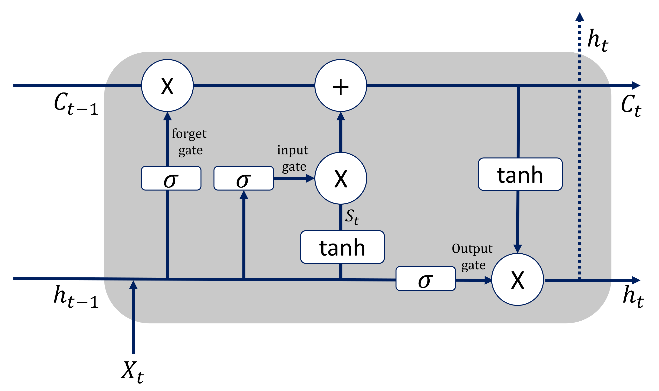
3.4. Long Short-Term Memory Model

The long short-term memory (LSTM) model is a variant of the recurrent neural network model that enables learning order dependence in sequential data [42]. The model was successfully applied for temporal and ordinal data, including image captioning, machine translation, and speech recognition [43,44,45]. Although the LSTM model works in similar steps to the recurrent neural network model, the procedures inside the cell are different. As shown in Figure 3, LSTM contains three main gates: input, output, and forget gates with internal memory. Each cell memorizes values in certain time intervals and these three gates control the information that comes in and out of the cell. The gates and internal memory of LSTM are used to resolve the vanishing and exploding gradient problems that often occur in recurrent neural network models.

The operational formulas of the LSTM method and definitions of notation are as follows:

$$f_t=\sigma (W_f{X}_t+U_f{h}_{t-1}+b_f)$$

(43)

$$i_t=\sigma (W_i{X}_t+U_i{h}_{t-1}+b_i)$$

(44)

$$o_t=\sigma (W_o{X}_t+U_o{h}_{t-1}+V_o{C}_t+b_o)$$

(45)

$$S_t=\tanh (W_c{X}_t+U_c{h}_{t-1}+b_c)$$

(46)

$$C_t=i_t{S}_t+f_{t-1}{S}_t$$

(47)

$$h_t=o_t\tanh (C_t)$$

(48)

• $X_t$ is the input vector to the memory cell at time $t$.
• $\sigma$ is the sigmoid function.
• $b$ is the bias vector.
• $W$, $U$ and $V$ are weight matrices.
• $i_t$, $f_t$, and $o_t$ are the values of the input, forget, and output gates at time $t$, respectively.
• $S_t$, $C_t$, and $h_t$ are the values of candidate state of the memory cell, the state of the memory cell at time $t$, and the value of the memory cell at time $t$, respectively.

The sigmoid function, $\sigma$ in Equations (43)–(45) generates values from zero to one. A value of one signifies that the input data are available to transfer through the gate, while the value of zero implies the opposite [43,46]. $S_t$ via tanh function in Equation (46) produces a new value at time $t$, which ranges from −1 to 1. The value of $C_t$ in Equation (47) is obtained from the inputs of $i_t$ and $f_t$, and the multiplication between $o_t$ and $\tanh (C_t)$ in Equation (48) results in the final output, $h_t$.

The LSTM model showed the best performance compared to the other machine learning methods for GHI prediction. Rajagukguk et al. [43] mentioned that the RMSE of the LSTM model ranged from 108.88 W/m² to 30.21 W/m², depending on location, input parameter, forecast horizon, and time interval. Thus, this study applied LSTM for solar irradiance forecasting in order to compare it with semi-empirical models, which contain regression equations. The inputs for the LSTM model were $C_{sat}$, ${\mathsf{\theta }}_{\mathrm{z}}$, $T_L$, and $\mathsf{\psi }$, whereas the constant value of $\mathrm{z}$ was ignored. The data from January–September 2018 were used for training, and those from October–December 2018 were selected for data tests.

3.5. Error Metrics for Model Validation

Determining statistical accuracy is necessary to quantify whether a model underestimates or overestimates the GHI. This study validated the accuracy through MBE, RMSE, rRMSE, and rMBE determination. The formulas were defined, respectively, as follows:

$$\mathrm{MBE}=\raisebox{1ex}{$1$}\!\left/ \!\raisebox{-1ex}{$n$}\right.{\displaystyle {\sum }_{i=1}^n({\mathrm{GHI}}_{\mathrm{model}}-{\mathrm{GHI}}_{\mathrm{measurement}})}$$

(49)

$$\mathrm{RMSE}=\sqrt{\raisebox{1ex}{$1$}\!\left/ \!\raisebox{-1ex}{$n$}\right.{{\displaystyle {\sum }_{i=1}^n({\mathrm{GHI}}_{\mathrm{model}}-{\mathrm{GHI}}_{\mathrm{measurement}})}}^2}$$

(50)

$$\mathrm{rRMSE}=\frac{\sqrt{\raisebox{1ex}{$1$}\!\left/ \!\raisebox{-1ex}{$n$}\right.{{\displaystyle {\sum }_{i=1}^n({\mathrm{GHI}}_{\mathrm{model}}-{\mathrm{GHI}}_{\mathrm{measurement}})}}^2}}{\raisebox{1ex}{$1$}\!\left/ \!\raisebox{-1ex}{$n$}\right.{\displaystyle {\sum }_{i=1}^n{\mathrm{GHI}}_{\mathrm{measurement}}}}\times 100$$

(51)

$$\mathrm{rMBE}=\frac{\raisebox{1ex}{$1$}\!\left/ \!\raisebox{-1ex}{$n$}\right.{\displaystyle {\sum }_{i=1}^n({\mathrm{GHI}}_{\mathrm{model}}-{\mathrm{GHI}}_{\mathrm{measurement}})}}{\raisebox{1ex}{$1$}\!\left/ \!\raisebox{-1ex}{$n$}\right.{\displaystyle {\sum }_{i=1}^n{\mathrm{GHI}}_{\mathrm{measurement}}}}\times 100,$$

(52)

where $n$ denotes the total number of data points. The RMSE indicated how close the predicted values were to the observational data with help from a regression line. The RMSE always produces a positive value. On the other hand, the MBE demonstrates the average bias in a model. The MBE is a sum of predicted data minus the observations. Hence, a positive MBE value indicates an overprediction, whereas a negative one represents an underprediction.

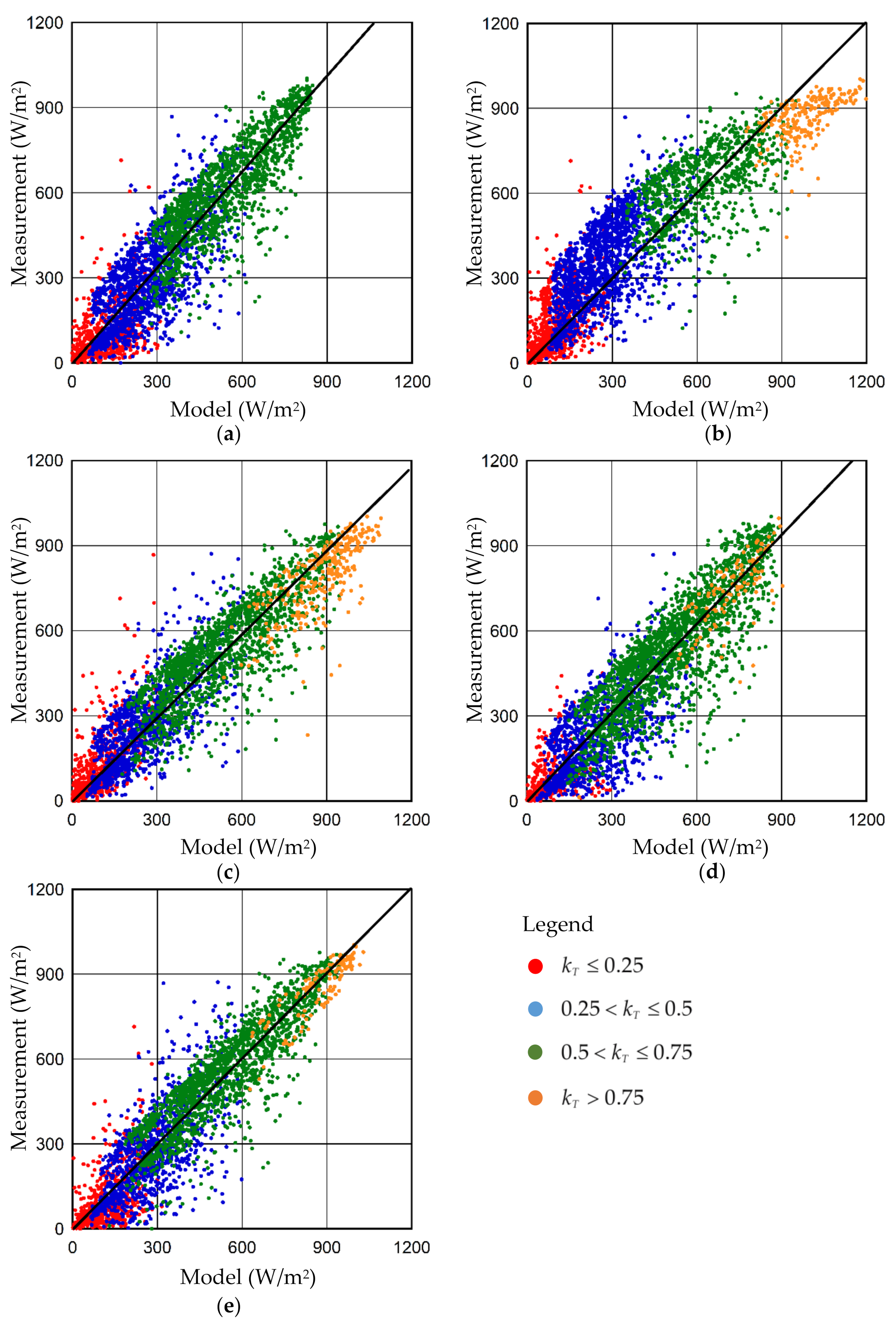
4. Results and Discussion

The vital step in determining CI is the pixel normalization to compensate for backscatter and air mass effects, which often create bias in images. Thus, the normalization provides the “true” brightness of the earth’s surface. Note that the digital number for COMS pixels varies from 0 to 1023. Figure 4 presents box-and-whisker plots of the pixel values after the normalization of each model was conducted. The normalized pixels were expected to demonstrate a constant dynamic range of the upper and lower boundaries. In all the models, the lower boundary was relatively constant, except at low backscatter angles. In other words, when the backscatter angle reached 0°, i.e., the sun was close to the satellite, the lower boundary tends to become slightly increased. The constant lower boundary indicates that the albedo for the earth’s surface had not change significantly. The upper boundaries, which represent overcast conditions, were also expected to remain constant. The variations of the upper boundaries were larger than those of the lower boundaries. Moreover, large maximums and some outliers beyond the maximum appeared. Consequently, the determination of the upper boundaries is more uncertain, and the GHI estimation under overcast conditions tends to be less accurate. Compared to the other three models, the Beyer model exhibited large deviations in terms of the interquartile range and the maximum. Based on the range of the normalized pixel counts, as shown in Figure 4, CI was determined according to Equation (1). CI indicates an attenuation factor from clear-sky GHI.

The derivations of ${\mathrm{GHI}}_c$ against $\mathsf{\gamma }$ are visualized in Figure 5. In general, all the models showed similar trends, where ${\mathrm{GHI}}_c$ escalated along with $\mathsf{\gamma }$. However, each model also yielded different dispersions due to their basic formulas. As previously discussed, the Beyer model does not consider atmospheric conditions via $T_L$. Consequently, the dispersion of the Beyer model results was the smallest among the models. The Rigollier and Hammer models produced a similar trend, while the latter showed slightly larger dispersions. Contrarily, the dispersion in the Perez and hybrid models was significantly wide. Note that a small or large dispersion does not imply that the ${\mathrm{GHI}}_c$ has good accuracy. Instead, it indicates that $T_L$ has significant effects in those two models. The maximum and minimum values of ${\mathrm{GHI}}_c$ also varied among the models. The Beyer model yielded the smallest range, from 70.22 to 859.54 W/m². The hybrid and Perez models produced broader ranges, of 10.12–1021.77 W/m² and 5.86–998.23 W/m², respectively. The Hammer model obtained the largest ${\mathrm{GHI}}_c$, where it achieved from 50.78 W/m² to 1092.52 W/m².

Based on CI and clear-sky irradiance, as shown in Figure 4 and Figure 5, GHI values under all sky conditions were derived and compared with the measurement data in Figure 6. The comparison was distinguished on different levels of the clearness index $(k_T={\mathrm{GHI}}_{\mathrm{model}}/I_0\cos {\mathsf{\theta }}_{\mathrm{z}})$. Note that $k_T\le 0.25$, $0.25<k_T\le 0.5$, $0.5<k_T\le 0.75$, and $k_T>0.75$ were described as cloudy, partially cloudy, clear, and clearest sky conditions, respectively. The scatterplots in Figure 6 indicate that all the semi-empirical models worked well within a $k_T$ range from 0.25 to 0.75. The Beyer model, the simplest model, was unable to estimate the GHI when $k_T>0.75$. It is obvious that the Rigollier model underestimates when $k_T$ is small, and the opposite when $k_T$ is large.

Error metrics for the comparisons in Figure 6 are summarized in

Table 6. Accuracy of the GHI models by level of clearness index.

Model	Clearness Level	R2	RMSE (W/m2)	rRMSE (%)	MBE (W/m2)	rMBE (%)
Beyer	$k_T\le 0.25$	0.60	87.23	90.29	10.25	10.61
	$0.25<k_T\le 0.5$	0.88	116.16	39.85	−26.86	−9.21
	$0.5<k_T\le 0.75$	0.97	121.59	19.65	−67.87	−10.97
	$k_T>0.75$	−	−	−	−	−
	All $k_T$	0.94	113.74	29.18	−36.84	−9.45
Rigollier	$k_T\le 0.25$	0.68	90.02	79.40	−30.26	−26.69
	$0.25<k_T\le 0.5$	0.88	145.46	41.45	−83.68	−23.85
	$0.5<k_T\le 0.75$	0.95	133.29	20.98	−12.83	−2.02
	$k_T>0.75$	0.99	145.97	16.85	121.16	13.98
	All $k_T$	0.91	137.38	35.09	−30.12	−7.69
Hammer	$k_T\le 0.25$	0.73	84.34	78.64	−21.65	−20.18
	$0.25<k_T\le 0.5$	0.87	105.56	40.14	−11.01	−4.18
	$0.5<k_T\le 0.75$	0.96	106.23	19.89	0.39	0.07
	$k_T>0.75$	0.98	126.50	15.88	90.87	11.41
	All $k_T$	0.94	103.92	26.54	0.09	0.02
Perez	$k_T\le 0.25$	0.52	84.73	89.46	−1.10	−1.16
	$0.25<k_T\le 0.5$	0.82	122.56	40.55	−16.96	−5.61
	$0.5<k_T\le 0.75$	0.96	111.29	20.46	−17.50	−3.21
	$k_T>0.75$	0.98	103.03	16.35	57.88	9.19
	All $k_T$	0.93	112.57	28.64	14.53	3.70
Hybrid	$k_T\le 0.25$	0.64	82.83	85.03	2.32	2.38
	$0.25<k_T\le 0.5$	0.85	113.39	40.90	−7.36	−2.65
	$0.5<k_T\le 0.75$	0.97	89.60	15.67	−19.17	−3.35
	$k_T>0.75$	0.99	48.24	5.47	10.06	1.14
	All $k_T$	0.95	97.08	24.12	−7.24	−1.80

. As indicated in Figure 6b, MBE values confirmed the biased estimation by the Rigollier model for different $k_T$ levels. The Hammer model also exhibited a similar trend to the Rigollier model, even though MBE values were reduced. Probably, the change from underestimation to overestimation as $k_T$ increases is a common feature of Helisat-2 models. On the other hand, RMSE generally decreases with $k_T$, which implies difficulties in generating accurate CI or limitations of CI-based modeling.

The accuracy for all sky conditions means the annual performance throughout 2018. All the models yielded promising results, in which they did not exceed 35.09% of rRMSE and −9.45% of rMBE. It was found that the Hammer model outperformed the other three semi-empirical models, with the best agreement of RMSE and MBE, as 103.92 W/m² and 0.09 W/m², respectively. Despite the fact that the Hammer model performed the best, the differences in accuracy among the Hammer, Perez, and Beyer models were small. The deviation in the rRMSE between the Hammer and Perez models was only 2.1%, whereas that between the Hammer and Beyers models was only 2.64%. In contrast, the Beyer model exhibited the largest MBE, with the value reaching −36.84 W/m².

The hybrid model had slightly improved RMSE and rRMSE compared to the Hammer model, with the differences of 6.84 W/m² and 2.42%, respectively. Meanwhile, the MBE and rMBE of the hybrid model were slightly larger than those of the Hammer model, with the absolute differences 7.15 W/m² and 1.82%, respectively. However, the rMBE of the Hammer model significantly varies with $k_T$, such that rMBE exceeds −20% when $k_T\le 0.25$. The rMBE of the hybrid model is fairly constant regardless of $k_T$ under the maximum absolute value of 3.35%. The separation of ${\mathrm{GHI}}_c$ into ${\mathrm{DNI}}_c$ and ${\mathrm{DHI}}_c$, such as in Rigollier and Hammer models (refer to Table 3) does not guarantee better accuracy. As shown in Table 6, the Hammer and Rigollier models demonstrated contrasting accuracies, either very good or very poor, in this study. Although the Beyer model adopted a very simple formula that does not address atmospheric conditions via $T_L$, it produced better accuracy than the Rigollier model. The hybrid model also took advantage of a simple clear-sky irradiance formula and improved accuracy. As a result, a simple model can be better than a complicated one if the clear-sky model is not sufficiently accurate.

Figure 7 shows variations of solar irradiance under clear-sky and overcast conditions on exemplary days. In general, all the semi-empirical models were capable of estimating hourly variations. However, all the models consistently overestimated or underestimated, for instance, for the morning on 9 April, afternoon on 9 April, morning on 2 December, and so on. Such consistent estimations, regardless of model, demonstrate that either the atmospheric data to produce clear-sky irradiance are inaccurate or the assumption that only the cloud amount contributes to reducing solar irradiance is incorrect. Pollen and yellow sand dust often occur during the spring season in Korea, but clear-sky irradiance models in Table 3 may not suitably account for such regional features. More importantly, rain and snow are likely to affect solar irradiance. As evidenced by large RMSE values when $k_T$ is low from Table 6, the consideration of the effects of rain and snow can improve model accuracy.

In order to investigate seasonal variations of model performance, monthly rRMSE and rMBE were plotted in Figure 8 and Figure 9. Even though seasonal variations of rRMSE are not so noticeable in Figure 8, prediction accuracy was slightly better in the spring and fall seasons. Probably, the reason was that sky in both of the seasons tends to be clear in Korea. Unlike rRMSE in Figure 8, rMBE in Figure 9 reveals remarkable seasonal variations independent of the model. Except for the Beyer model, overestimation only occurs during the summer season. The closer to the winter season the time gets, the larger the underestimation becomes. This seasonal change of accuracy is caused by ground albedo change [2,47]. The location of interest, i.e., Kookmin University, is adjacent to the mountain, and the 1 × 1-km² COMS pixel corresponding to the location is likely to include both buildings and forest. Consequently, the combined effects of vegetation, soil, and building properties resulted in the ground albedo, $C_{\min }$. In winter, this issue becomes even more evident due to snow cover, which is often disguised as cloud. If the ground albedo change is considered, the solar irradiance model can improve prediction accuracy.

The Rigollier model consistently produced the largest error, and it only performed slightly better than the Beyer model during April and September 2018. Contrarily, the Hammer model produced smaller rRMSE and rMBE values than the Beyer, Perez, and Rigollier models throughout the 12 months. The lowest errors gained by the Hammer model were 18.8% for the rRMSE and 0.6% for the rMBE in April. The accuracy of the Perez model followed that of the Hammer model, with the best rRMSE and rMBE being 22.6% in February and 3.7% in September, respectively. The hybrid model consistently had a better accuracy than any of the four semi-empirical models for each month, with the lowest rRMSE and rMBE values at 17.1% and −0.1% during April, respectively. The hybrid model also showed higher accuracy compared with the other models during winter, as can be observed from the rRMSE values of 19.9%, 21.4%, and 18.5% for December, January, and February, respectively.

So far, the hybrid model has turned out to be more accurate than any other model. However, the development of such models is cumbersome and awkward because the hybrid model in this study was created after using trial-and-error combinations of constituent formulas. Therefore, to replace the combination process in the hybrid model, an LSTM model was attempted, and its results are summarized in

Table 7. Accuracy of the semi-empirical models and LSTM model from October to December 2018.

Model	RMSE (W/m2)	rRMSE (%)	MBE (W/m2)	rMBE (%)
Beyer	118.95	28.10	−88.05	−20.80
Rigollier	143.45	41.09	−107.27	−30.72
Hammer	88.36	25.31	−35.44	−10.15
Perez	89.67	25.75	−28.71	−8.24
Hybrid	86.14	23.92	−19.70	−5.47
LSTM	76.45	21.92	−24.28	−6.96

. As the hybrid model produced the best accuracy among the semi-empirical models, the input variables of the hybrid model ($C_{sat}$, ${\mathsf{\theta }}_{\mathrm{z}}$, $T_L$, and $\mathsf{\psi }$) were selected for those of the LSTM model. The LSTM model revealed a slight improvement in RMSE compared to the hybrid model. Its MBE slightly increased, but it was comparable to that of the hybrid model and still better than those of the other models. Consequently, it was demonstrated that the machine learning method can replace the hybrid model.

5. Conclusions

Four semi-empirical models that use pixel values from a COMS geostationary satellite in order to extract GHI were evaluated. The models were compared using the same data time-resolution and location. The investigation was also deepened by separating the GHI based on daily, monthly, and annual evaluations, as well as on a clearness index. This study demonstrated that the Hammer model was selected as the most appropriate model for deriving the GHI over Korea, according to the RMSE and MBE.

The hybrid model, which was developed from the combination of correlation formulas, was found to exhibit moderately improved accuracy and successfully simplified a lengthy procedure in the Hammer and Rigollier models. The hybrid model was also able to slightly decrease the RMSE and rRMSE of the Hammer model from 103.92 W/m² and 26.54%, to 97.08 W/m² and 24.12%, respectively.

In order to replace the trial-and-error combination of the hybrid model, a machine learning model of LSTM was also presented. The LSTM model was able to predict GHI more accurately than the hybrid model, with an enhancement in rRMSE of 2%, although its rMBE was still comparable to that of the hybrid model.

Semi-empirical models can accurately determine the GHI with a small number of inputs, such as ${\mathsf{\theta }}_{\mathrm{z}}$, $\mathsf{\phi }$, $T_L$, $\mathsf{\psi }$, and $\mathrm{z}$. In the context of Korea, this study provided a comparison of well-known semi-empirical models and suggested improved methods using hybrid formulas and the LSTM method. Hopefully, this study will be helpful for utilizing a semi-empirical approach to estimating solar irradiance in regions with a hot summer continental climate.

References

1. Ineichen, P.; Perez, R. Derivation of Cloud Index from Geostationary Satellites and Application to the Production of Solar Irradiance and Daylight Illuminance Data. Theor. Appl. Climatol. 1999, 64, 119–130. [Google Scholar] [CrossRef]
2. Perez, R.; Ineichen, P.; Moore, K.; Kmiecik, M.; Chain, C.; George, R.; Vignola, F. A New Operational Model for Satellite-Derived Irradiances: Description and Validation. Sol. Energy 2002, 73, 307–317. [Google Scholar] [CrossRef]
3. Rigollier, C.; Lefèvre, M.; Wald, L. The Method Heliosat-2 for Deriving Shortwave Solar Radiation from Satellite Images. Sol. Energy 2004, 77, 159–169. [Google Scholar] [CrossRef]
4. Yang, L.; Gao, X.; Hua, J.; Wu, P.; Li, Z.; Jia, D. Very Short-Term Surface Solar Irradiance Forecasting. Sensors 2020, 20, 2606. [Google Scholar] [CrossRef]
5. Zelenka, A.; Perez, R.; Seals, R.; Renné, D. Effective Accuracy of Satellite-Derived Hourly Irradiances. Theor. Appl. Climatol. 1999, 62, 199–207. [Google Scholar] [CrossRef]
6. Mouhamet, D.; Tommy, A.; Primerose, A.; Laurent, L. Improving the Heliosat-2 Method for Surface Solar Irradiation Estimation under Cloudy Sky Areas. Sol. Energy 2018, 169, 565–576. [Google Scholar] [CrossRef]
7. National Renewable Energy Laboratory National Solar Radiation Database 1991–2005 Update: User’s Manual. Task No. PVA7.6102; National Renewable Energy Lab.: Golden, CO, USA, 2007; Available online: https://www.nrel.gov/docs/fy07osti/41364.pdf (accessed on 12 April 2021). [CrossRef]
8. Hammer, A.; Heinemann, D.; Hoyer, C.; Kuhlemann, R.; Lorenz, E.; Müller, R.; Beyer, H.G. Solar Energy Assessment Using Remote Sensing Technologies. Remote Sens. Environ. 2003, 86, 423–432. [Google Scholar] [CrossRef]
9. Cano, D.; Monget, J.M.; Albuisson, M.; Guillard, H.; Regas, N.; Wald, L. A Method for the Determination of the Global Solar Radiation from Meteorological Satellite Data. Sol. Energy 1986, 37, 31–39. [Google Scholar] [CrossRef]
10. Beyer, H.G.; Costanzo, C.; Heinemann, D. Modifications of the Heliosat Procedure for Irradiance Estimates from Satellite Images. Sol. Energy 1996, 56, 207–212. [Google Scholar] [CrossRef]
11. Moradi, I.; Mueller, R.; Alijani, B.; Kamali, G.A. Evaluation of the Heliosat-II Method Using Daily Irradiation Data for Four Stations in Iran. Sol. Energy 2009, 83, 150–156. [Google Scholar] [CrossRef]
12. Eissa, Y.; Chiesa, M.; Ghedira, H. Assessment and Recalibration of the Heliosat-2 Method in Global Horizontal Irradiance Modeling over the Desert Environment of the UAE. Sol. Energy 2012, 86, 1816–1825. [Google Scholar] [CrossRef]
13. Janjai, S.; Sricharoen, K.; Pattarapanitchai, S. Semi-Empirical Models for the Estimation of Clear Sky Solar Global and Direct Normal Irradiances in the Tropics. Appl. Energy 2011, 88, 4749–4755. [Google Scholar] [CrossRef]
14. Sengupta, M.; Heidinger, A.; Miller, S. Validating an Operational Physical Method to Compute Surface Radiation from Geostationary Satellites. Reliab. Photovolt. Cells Modul. Compon. Syst. III 2010, 7773, 77730T. [Google Scholar] [CrossRef]
15. Seok, C.W.; Ram, S.A.; Yong, K. Solar Irradiance Estimation in Korea by Using Modified Heliosat-II Method and COMS-MI Imagery. J. Korean Soc. Surv. Geod. Photogramm. Cartogr. 2015, 33, 463–472. [Google Scholar] [CrossRef]
16. Jia, D.; Hua, J.; Wang, L.; Guo, Y.; Guo, H.; Wu, P.; Liu, M.; Yang, L. Estimations of Global Horizontal Irradiance and Direct Normal Irradiance by Using Fengyun-4a Satellite Data in Northern China. Remote Sens. 2021, 13, 790. [Google Scholar] [CrossRef]
17. Yeom, J.M.; Han, K.S.; Kim, J.J. Evaluation on Penetration Rate of Cloud for Incoming Solar Radiation Using Geostationary Satellite Data. Asia Pac. J. Atmos. Sci. 2012, 48, 115–123. [Google Scholar] [CrossRef]
18. Lefèvre, M.; Oumbe, A.; Blanc, P.; Espinar, B.; Gschwind, B.; Qu, Z.; Wald, L.; Schroedter-Homscheidt, M.; Hoyer-Klick, C.; Arola, A.; et al. McClear: A New Model Estimating Downwelling Solar Radiation at Ground Level in Clear-Sky Conditions. Atmos. Meas. Tech. 2013, 6, 2403–2418. [Google Scholar] [CrossRef]
19. Zo, I.S.; Jee, J.B.; Lee, K.T.; Kim, B.Y. Analysis of Solar Radiation on the Surface Estimated from GWNU Solar Radiation Model with Temporal Resolution of Satellite Cloud Fraction. Asia Pac. J. Atmos. Sci. 2016, 52, 405–412. [Google Scholar] [CrossRef]
20. Qu, Z.; Oumbe, A.; Blanc, P.; Espinar, B.; Gesell, G.; Gschwind, B.; Klüser, L.; Lefèvre, M.; Saboret, L.; Schroedter-Homscheidt, M.; et al. Fast Radiative Transfer Parameterisation for Assessing the Surface Solar Irradiance: The Heliosat-4 Method. Meteorol. Z. 2017, 26, 33–57. [Google Scholar] [CrossRef]
21. Xie, Y.; Sengupta, M.; Dudhia, J. A Fast All-Sky Radiation Model for Solar Applications (FARMS): Algorithm and Performance Evaluation. Sol. Energy 2016, 135, 435–445. [Google Scholar] [CrossRef]
22. Yeom, J.M.; Seo, Y.K.; Kim, D.S.; Han, K.S. Solar Radiation Received by Slopes Using COMS Imagery, a Physically Based Radiation Model, and GLOBE. J. Sens. 2016, 2016, 4834579. [Google Scholar] [CrossRef]
23. Kim, C.K.; Kim, H.-G.; Kang, Y.-H.; Yun, C.-Y.; Lee, S.-N. Evaluation of Global Horizontal Irradiance Derived from CLAVR-x Model and COMS Imagery Over the Korean Peninsula. New Renew. Energy 2016, 12, 13. [Google Scholar] [CrossRef]
24. Carver, S.; Mikkelsen, N.; Woodward, J. Updated World Map of the Köppen-Geiger Climate Classification. Permafr. Periglac. Process. 2002, 13, 243–249. [Google Scholar] [CrossRef]
25. Ascencio-Vásquez, J.; Brecl, K.; Topič, M. Methodology of Köppen-Geiger-Photovoltaic Climate Classification and Implications to Worldwide Mapping of PV System Performance. Sol. Energy 2019, 191, 672–685. [Google Scholar] [CrossRef]
26. Kawamura, H.; Tanahashi, S.; Takahashi, T. Estimation of Insolation over the Pacific Ocean off the Sanriku Coast. J. Oceanogr. 1998, 54, 457–464. [Google Scholar] [CrossRef]
27. EKO Instrument Co., Ltd. MS-57 Instruction Manual Pyrheliometer Ver. 3; Version 3; EKO Instrument Co., Ltd.: Tokyo, Japan, 2019. [Google Scholar]
28. EKO Instrument Co., Ltd. MS-802 Instruction Manual Pyranometer Ver. 3; Version 3; EKO Instrument Co., Ltd.: Tokyo, Japan, 2019. [Google Scholar]
29. Gueymard, C.A.; Ruiz-Arias, J.A. Extensive Worldwide Validation and Climate Sensitivity Analysis of Direct Irradiance Predictions from 1-Min Global Irradiance. Sol. Energy 2016, 128, 1–30. [Google Scholar] [CrossRef]
30. Emery, W.; Camps, A. Introduction to Satellite Remote Sensing: Atmosphere, Ocean, Land, and Cryosphere Applications; Elsevier: Amsterdam, The Netherlands, 2017. [Google Scholar] [CrossRef]
31. Kumar, K.R.; Sivakumar, V.; Reddy, R.R.; Gopal, K.R.; Adesina, A.J. Inferring Wavelength Dependence of AOD and Ångström Exponent over a Sub-Tropical Station in South Africa Using AERONET Data: Influence of Meteorology, Long-Range Transport and Curvature Effect. Sci. Total Environ. 2013, 461–462, 397–408. [Google Scholar] [CrossRef]
32. Rigollier, C.; Bauer, O.; Wald, L. On the Clear Sky Model of the ESRA—European Solar Radiation Atlas—With Respect to the Heliosat Method. Sol. Energy 2000, 68, 33–48. [Google Scholar] [CrossRef]
33. Kasten, F. Parametriesirung Der Globalstahlung Durch Bedeckungsgrad Und Trubungsfaktor. Ann. Meteorol. Neue Folge 1984, 20, 49–50. [Google Scholar]
34. Diabaté, L.; Demarcq, H.; Michaud-Regas, N.; Wald, L. Estimating Incident Solar Radiation at The Surface from Images of The Earth Transmitted by Geostationary Satellites: The Heliosat Project. Int. J. Sol. Energy 1987, 5, 261–278. [Google Scholar] [CrossRef]
35. Song, A.; Choi, K.; Jung, M.; Kim, Y. Estimation of the Linke Turbidity Factor and the Solar Irradiance under a Clear Sky Over the Korean Peninsula Using COMS MI. New Renew. Energy 2016, 12, 21. [Google Scholar] [CrossRef]
36. Ineichen, P.; Perez, R. A New Airmass Independent Formulation for the Linke Turbidity Coefficient. Sol. Energy 2002, 73, 151–157. [Google Scholar] [CrossRef]
37. Marif, Y.; Bechki, D.; Zerrouki, M.; Belhadj, M.M.; Bouguettaia, H.; Benmoussa, H. Estimation of Atmospheric Turbidity over Adrar City in Algeria. J. King Saud Univ. Sci. 2019, 31, 143–149. [Google Scholar] [CrossRef]
38. Bourges, G. Courbes de Fréquence Cumulées de l’irradiation Solaire Globale Horaire Reçue Par Une Surface Plane; Tome II; European Commission: Brussels, Luxembourg, 1979. [Google Scholar]
39. Page, J. Algorithms for The Satellight Programme; Projektinterner Berict; 1996. [Google Scholar]
40. Jacovides, C.P. Model Comparison For The Calculation of Linke’s Turbidity Factor. Int. J. Climatol. 1997, 17, 551–563. [Google Scholar] [CrossRef]
41. Remund, J.; Wald, L.; Lefevre, M.; Ranchin, T.; Page, J.; Remund, J.; Wald, L.; Lefevre, M.; Ranchin, T.; Page, J.; et al. Worldwide Linke Turbidity Information. In Proceedings of the ISES Solar World Congress, Göteborg, Sweden, 14–19 June 2003. [Google Scholar] [CrossRef]
42. Hochreiter, S.; Schmidhuber, J. Long Short-Term Memory. Neural Comput. 1997, 9, 1735–1780. [Google Scholar] [CrossRef]
43. Rajagukguk, R.A.; Ramadhan, R.A.A.; Lee, H.-J. A Review on Deep Learning Models for Forecasting Time Series Data of Solar Irradiance and Photovoltaic Power. Energies 2020, 13, 6623. [Google Scholar] [CrossRef]
44. Aslam, M.; Lee, J.M.; Kim, H.S.; Lee, S.J.; Hong, S. Deep Learning Models for Long-Term Solar Radiation Forecasting Considering Microgrid Installation: A Comparative Study. Energies 2019, 13, 147. [Google Scholar] [CrossRef]
45. Husein, M.; Chung, I.Y. Day-Ahead Solar Irradiance Forecasting for Microgrids Using a Long Short-Term Memory Recurrent Neural Network: A Deep Learning Approach. Energies 2019, 12, 1856. [Google Scholar] [CrossRef]
46. Jeon, B.K.; Kim, E.J. Next-Day Prediction of Hourly Solar Irradiance Using Local Weather Forecasts and LSTM Trained with Non-Local Data. Energies 2020, 13, 5258. [Google Scholar] [CrossRef]
47. Choi, W.; Song, A.; Kim, Y. Estimation of Solar Radiation by Using Modified Heliosat-II Method and COMS-MI Imagery. Remote Sens. Clouds Atmos. XX 2015, 9640, 964015. [Google Scholar] [CrossRef]
Figure 1. Example of a satellite image from visible channel provided by COMS (Communication, Ocean, and Meteorological Satellite), stationed at 36,000 km above the equator. This image is considered as level 1B data.
Applsci 11 03445 g001
Figure 2. Procedure to derive solar irradiance from satellite images.
Applsci 11 03445 g002
Figure 3. Architecture of the long short-term memory (LSTM).
Applsci 11 03445 g003
Figure 4. Normalized COMS satellite pixel against backscatter angle; (a) Beyer, (b) Rigollier, (c) Hammer, (d) Perez, and (e) hybrid models. The backscatter angle, ψ , was divided into nine classes with the interval of 10°. In the box-and-whisker plot, the box height is the distance between the first and the third quartiles, and the maximum and minimum is determined by the interquartile range.
Applsci 11 03445 g004
Figure 5. Clear-sky irradiance against the sun elevation angle; (a) Beyer, (b) Rigollier, (c) Hammer, (d) Perez, and (e) hybrid models. The sun elevation angle, γ , was divided into eight classes with the interval of 10°.
Applsci 11 03445 g005
Figure 6. Comparison of modeling results with measurement data by the level of the clearness index; (a) Beyer, (b) Rigollier, (c) Hammer, (d) Perez, and (e) hybrid models. The clearness index, k T , was divided into four classes with the interval of 0.25.
Applsci 11 03445 g006
Figure 7. Daily variations of solar irradiance: (a) clear sky conditions and (b) overcast conditions.
Applsci 11 03445 g007aApplsci 11 03445 g007b
Figure 8. Comparison of monthly accuracy based on rRMSE (%).
Applsci 11 03445 g008
Figure 9. Comparison of monthly accuracy based on rMBE (%).
Applsci 11 03445 g009