1. Introduction
Neural network design requires the proper determination of the input variables, i.e., the appropriate selection of the factors that affect the variable behavior to be modeled. However, this is not a trivial issue because there is no formal theory to ensure that the selected network is the best for a particular application problem. There are no handled performance metrics for unsupervised neural networks to ensure that the configuration developed has reached the optimal performance [
1]. In supervised neural networks, the Mean Absolute Percentage Error (MAPE) is commonly used to evaluate the generalization capability of the model. Likewise, the state-of-the-art reports that the Akaike information criterion (AIC) is proposed as a measure of comparison to identify a suitable configuration [
2,
3]. For these reasons, it is necessary to know which factors influence the behavior of these two-performance metrics, so that it can be established whether it is possible to determine an optimal operating point for AIC and an appropriate dispersion index level for MAPE.
Next, this paper will show some examples of the neural network training process design, applying different strategies.
The training process models based on Radial Basis Function (RBF) networks [
4] are the most efficient in the neural network models for achieving an effective, adaptive, and versatile architecture with precise computational time results. A multi-level neural architecture composed of RBF Serially Operating Multipliers (SOM) algorithms executed in parallel in a programming mode known as Compute Unified Device Architecture (CUDA) is proposed by [
5] to improve the accuracy and timing of the RBF model with the same amount of data. The validation for such a structure consists of estimating ecological variables with information on the environment through the CUDA-RBF-SOM structure, which shows an improvement in time and precision for the training process of 0.1154% compared with the RBF network for the same estimated variable. In conclusion, they present a new training process (CUDA-RBF-SOM) that reduces the execution time by 99.8846% compared to an RBF-SOM model.
In some cases, the quantity of data for the training process can lead to a problem, so the architecture must not be limited by data. The neural network model proposed by [
6] is focused on reducing the quantity of input data needed in the training process. An RBF network is applied to regression problems; the new structure consists of a multi-stage training process that matches the orthogonal least squares (OLS) with an optimization gradient. The model validation tests are performed on the data for the prediction of stress and force in the knee required to prevent injuries in different scenarios (tasks), in which the results and estimated times are compared with other models, such as OLS and feed-forward back-propagation network (FFN), with their real values. The proposed structure named Opt-RBN shows, in some scenarios, favorable results in the training data. Although the training process time is a little longer, the authors consider it a good time because it is less than one minute.
The Stochastic Gradient Descent (SGD) model during the training process updates a Convolutional Neural Network (CNN) with a noisy gradient calculated from a random batch. Each batch uniformly updates the network every once in a while, which leads to loss problems in the batches. A model to mitigate this problem is proposed in the form of a stochastic process that automatically selects the batch with the largest loss to accelerate its training. This is called Inconsistent Stochastic Gradient Descent (ISGD) by [
7]. The key concept is that the inconsistent training dynamically adjusts the training effort without loss. ISGD gradually reduces the average lost batch and uses a dynamic upper control limit to identify a large lost batch as it goes along. The ISGD remains in the identified batch to speed up the training with additional gradient updates. The tests for validating the ISGD are based on data such as those derived from ImageNet (A large-scale hierarchical image database), MNIST (Modified National Institute of Standards and Technology database), and CIFAR-10 (Canadian Institute For Advanced Research database). Those tests showed a convergence of the ISGD that was 14.94% faster than the SGD using the ImageNet database. ISGD showed a convergence that was 23.57% faster than the SGD in the CIFAR-10 test. It also showed a convergence that was 28.57% faster than the SGD using the MNIST database.
The Back Propagation Neural Network (BPNN) model is used in the training process to determine the number of neurons needed in the two hidden layers of a neural network to forecast the magnitude, on the Richter scale, of earthquakes in a region of the Philippine Sea [
8]. With the use of a data register for the earthquakes in the area from 1990 to 2014, several series of BPNN models were built to forecast the magnitude of the earthquake and compare them to the actual data. From the obtained data, it was concluded that a number of 10 neurons per hidden layer is the ideal number for the forecasting model, since the forecasting errors of the BPNN model with 10 neurons in each hidden layer were very similar to those of the models that use more than 10 neurons per layer, which involves a longer time of computation for similar results. The results were compared with the actual values of the magnitudes of earthquakes that have already occurred, and the authors concluded that the BPNN model forecasts a reliable Richter scale earthquake magnitude result.
Neural network models are used to solve the text categorization problem. One of the models is the Improved Back-Propagation Neural Network (IBPNN), proposed by [
9], that, with a parallel computational process, speeds up the neural network training for text categorization. The BPNN algorithm uses a Sun Cluster with 34 nodes (processors). The parallel IBPNN is integrated with the Singular Value Decomposition (SVD) technique, wherein the neural network input is represented as a low dimensional feature vector. The validation is performed using different databases wherein the number of processors is modified from 1 to 32, which produces an improvement in the execution time without diminishing the categorized text accuracy. The results show that the parallel IBPNN and the SVD technique achieve a faster, more adaptive, and more reliable training process in the text categorization problem.
Table 1 shows a summary of techniques commonly used in the training of time series models.
According to
Table 1, the data modeling process is not unique when evaluating several different configurations’ performances to select one that best fits the variables to be considered along with the data themselves. Depending on the configuration, it will be necessary to define which process is more suitable for adjusting each parameter that defines it. Since there is no formal theory for selecting the best model, in the case of neural networks, it is common to find authors who base their selection on iterative processes in which the training parameters change. The training process is supposed to be automatized, and an experimental design wherein the most significant parameters are identified within the modeling structure is proposed, in such a way that parameters change during the iterative process for selection and comparison.
2. Experimental Planification
A design for experiments considering AIC and MAPE as performance metrics is proposed to identify which factors are significant in the neural networks’ training process for forecasting purposes. The historical energy demand data of an energy commercialization market in Colombia, in the city of Barranquilla, were used to carry out this procedure [
16].
In the training process, the validation and selection of the neural network can influence the adaptability and generalization of the neural network. Factors related to the network configuration are highlighted in the first instance, within which are (1) network type, (2) number of layers, (3) the number of neurons in the hidden layer, and (4) activation function type. Additionally, the factors defined in the training and validation stages are (5) initial learning coefficient, (6) number of data to consider, (7) percentage of data for training, validation, and testing, (8) training algorithm, (9) training epochs, (10) corresponding time, and (11) presentation data order for training [
17].
Factors 1, 4, 9, 10, and 11 are held constant. The activation functions used in pattern recognition and classification are typically the input neurons′ identity function, and the sigmoid function for the other layers (hidden layer and output layer). For the network type, a Multilayer Perceptron (MLP) is used due to its better generalization capability; for example, RBF for activities related to classification and pattern recognition applications. The number of epochs is set at 100.
Factors 2, 3, and 5–9 will be the design factors manipulated to verify their significance in the AIC index and the MAPE metric. Since the main goal is to identify which factors are significant in designing a neural network for time series modeling, we decided to choose two factor levels (low and high).
According to the state-of-the-art, the ranges to be considered during the training and validation processes shall be as follows:
Training algorithm—Levenberg–Marquardt or Resilient Backpropagation;
Number of hidden layers—1–5;
Number of neurons in the hidden layer—1–10;
Data number—60–120;
Validation percentage—10–30.
Table 2 shows the levels and ranges for the design factors.
Since the objective of this study is to identify the significant factors in the performance of a neural network for forecasting purposes, we chose to select as response variables the AIC and the MAPE.
3. Experimental Design
The 2
k factorial design is selected to evaluate each factor’s effect on the neural network′s training and validation processes. This experiment is adequate when the goal is to analyze the significance of the factors with a minimum number of runs [
18]. In this case, only two levels (low and high) are considered. This can be viewed as a weakness when the factors have significant interaction and a curvature in the experimental zone. When the curvature is detected, it is necessary to aggregate central and axial points in the experimental design. Another aspect to consider is the null quantity of the degree of freedom of the error. Thus, it is recommended to apply the following two strategies: (1) to identify the significant effects through a normal probability plot, i.e., remove from the analysis those factors fitted to the normal probability plot because their behaviors are similar to the residues. In this case, the degree of freedom of each excluded effect is added to the error. (2) To aggregate central points to the 2
k experiment; these points are added in the center of the experimental zone, at points
. This strategy allows for adding a degree of freedom to the error and measuring the response variable experimental zone curvature.
The experimental design carried out in this paper is a 25 with six central points. Three of these will be developed with a qualitative factor in the low level (Levenberg–Marquardt algorithm) and the other three in the high level (Resilient Backpropagation algorithm). If the linear model does not fit the data, adding an axial point located at the central point will be necessary.
4. Experimental Results
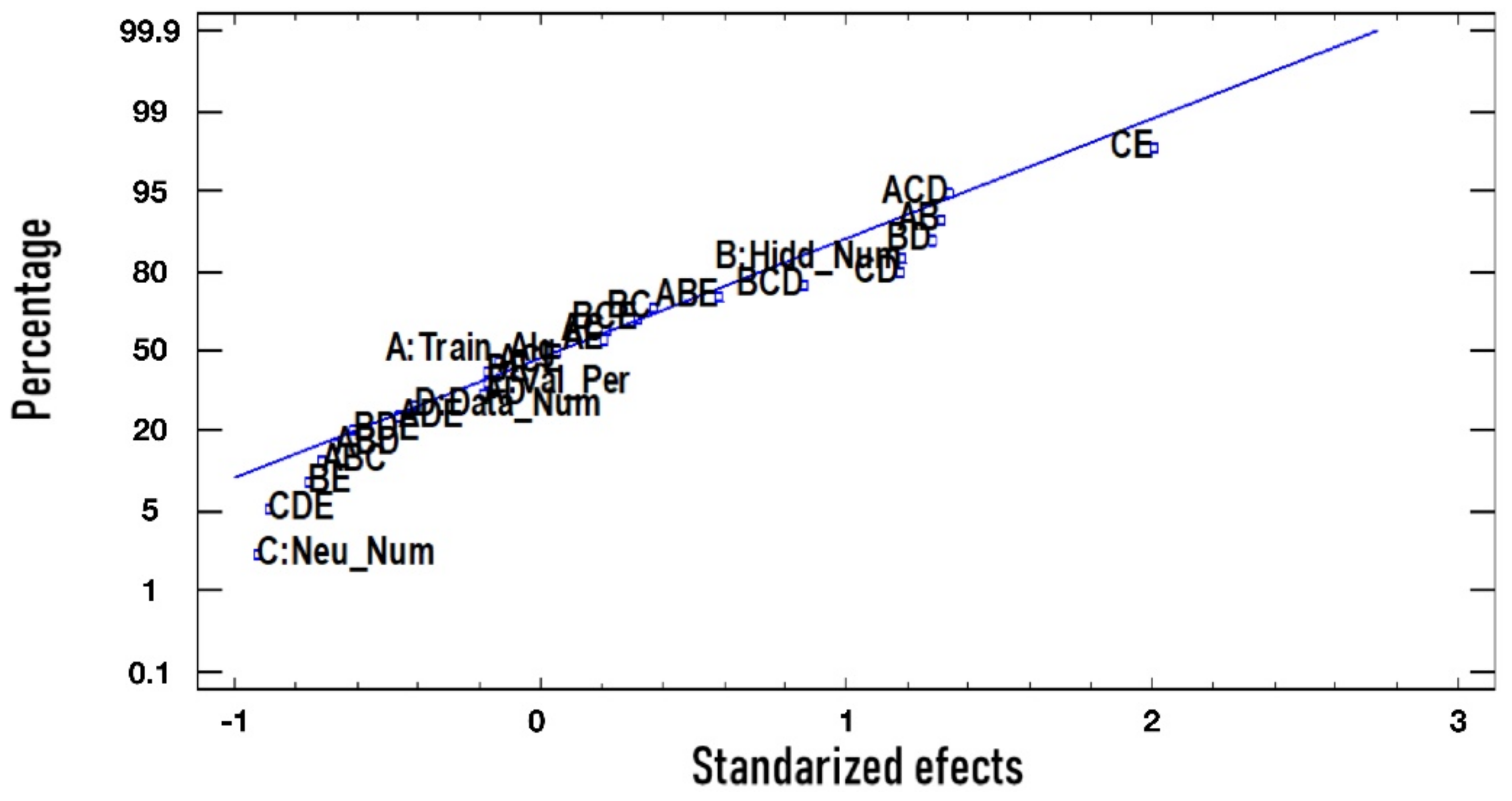
ANOVA multifactorial analysis of variance is used to identify which factors are relevant. In this sense, a normal probability plot is constructed to determine which factors are relevant, as shown in
Figure 1 for the AIC index.
Figure 1 and
Table 3 show the CE effect as the most relevant. The AIC response is only affected by the CE effect, because the
p-value is less than 0.05. It is necessary to verify that the model fulfills the normality, homoscedasticity, and independent conditions to validate the result reached through the ANOVA analysis.
Table 3 shows the results reached through the ANOVA analysis for AIC.
Table 3.
ANOVA for AIC.
| Source | Sum of Squares | Degrees of Freedom | Mean Square | F-Ratio | p-Value |
|---|
| A: Train_Alg | 24.1165 | 1 | 24.1165 | 0.00 | 0.9507 |
| B: Hidd_Num | 10,937.1 | 1 | 10,937.1 | 1.77 | 0.1968 |
| C: Neu_Num | 6739.35 | 1 | 6739.35 | 1.09 | 0.3074 |
| D: Data_Num | 1338.51 | 1 | 1338.51 | 0.22 | 0.6460 |
| E: Val_Per | 240.395 | 1 | 240.395 | 0.04 | 0.8454 |
| AB | 13,455.4 | 1 | 13,455.4 | 2.18 | 0.1540 |
| AC | 366.218 | 1 | 366.218 | 0.06 | 0.8098 |
| AD | 266.442 | 1 | 266.442 | 0.04 | 0.8373 |
| AE | 350.781 | 1 | 350.781 | 0.06 | 0.8138 |
| BC | 1048.89 | 1 | 1048.89 | 0.17 | 0.6842 |
| BD | 12,865.9 | 1 | 12,865.9 | 2.08 | 0.1629 |
| BE | 4542.03 | 1 | 4542.03 | 0.74 | 0.4003 |
| CD | 10,783.0 | 1 | 10,783.0 | 1.75 | 0.1999 |
| CE | 31,620.4 | 1 | 31,620.4 | 5.12 | 0.0338 |
| DE | 237.081 | 1 | 237.081 | 0.04 | 0.8464 |
| Total error | 135,813 | 22 | 6173.34 | | |
| Total (corrected error) | 230,629 | 37 | | | |
Because the Chi-square test has a p-value greater than 0.05, it is not possible to reject the null hypothesis; hence, the residuals fit into a normality plot.
To verify the homoscedasticity condition, we used the Levene’s test, as shown in
Table 5.
According to the results in
Table 5, four factors fulfill the homoscedasticity condition because their
p-values are greater than 0.05.
The third and last condition is lag 1 autocorrelation, and the results are as follows: Durbin–Watson = 2.3533 (p-value = 0.5515), Lag 1 autocorrelation = −0.057753. The Durbin–Watson statistic is equal to 2 approximately; hence, residuals are independent.
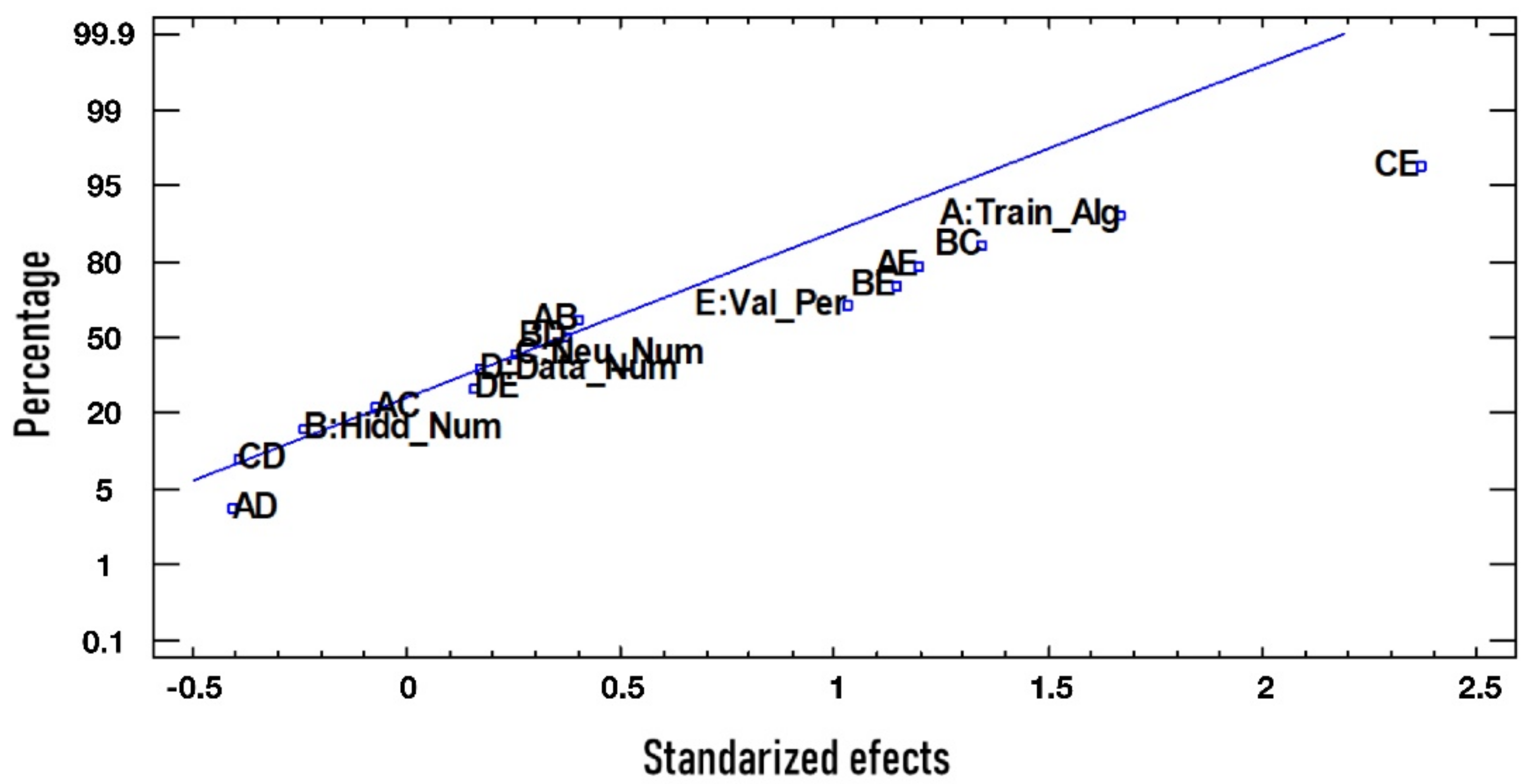
For MAPE analysis the same procedure is carried out. As is seen in
Figure 2 and
Table 6, the CE effect is the most relevant. The MAPE response is only affected by the CE effect, because the
p-value is less than 0.05. It is necessary to verify that the model fulfills the normality, homoscedasticity, and independent conditions to validate the result reached through the ANOVA analysis for MAPE.
Chi-square is used to validate the normality condition. The result is shown in
Table 7.
There are no data results for this stage with the normality test. Since the factors have similar effects compared to the AIC response, it is considered acceptable to continue the optimization stage with only the last response variable.
According to the results of
Table 8, four factors fulfill the homoscedasticity condition because the
p-values are greater than 0.05.
Durbin–Watson statistic = 2.13134 (p-value = 0.6651), and Lag 1 residual autocorrelation = −0.158786.
Due to the fact that the Durbin–Watson statistic has a p-value greater than 0.05, the null hypothesis is rejected; hence, the residuals have no linear correlation.
5. Regression Model
According to the ANOVA analysis, the interaction of two factors (C: Neurons number and E: Validation percentage) is related significantly to the AIC behavior. Now, it is necessary to set an ideal configuration through an optimization process. To carry out this stage, the experimental design to be used is two factors with one replicate.
The results of the experiment are shown in
Table 9.
Equation (1) shows the fitted equation of the regression model for the AIC response. The coefficient test is conducted according to the result shown in
Table 10.
Table 11 shows the grouped regression statistics of the adjusted model. The R
2 is the achieved correlation coefficient.
Table 12 shows that the
p-value (4.7736 × 10
−7) is less than the α used in the experiment; hence, the null hypothesis is rejected, demonstrating that the model fits to the actual data.
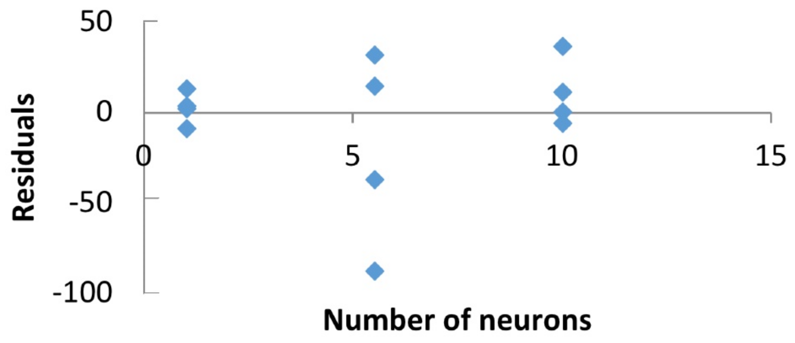
Figure 3 shows only the residuals for the relevant factor (number of neurons) discovered in the fitting curve for the AIC response. It has no clear structure in the residuals data.
6. Optimization Results
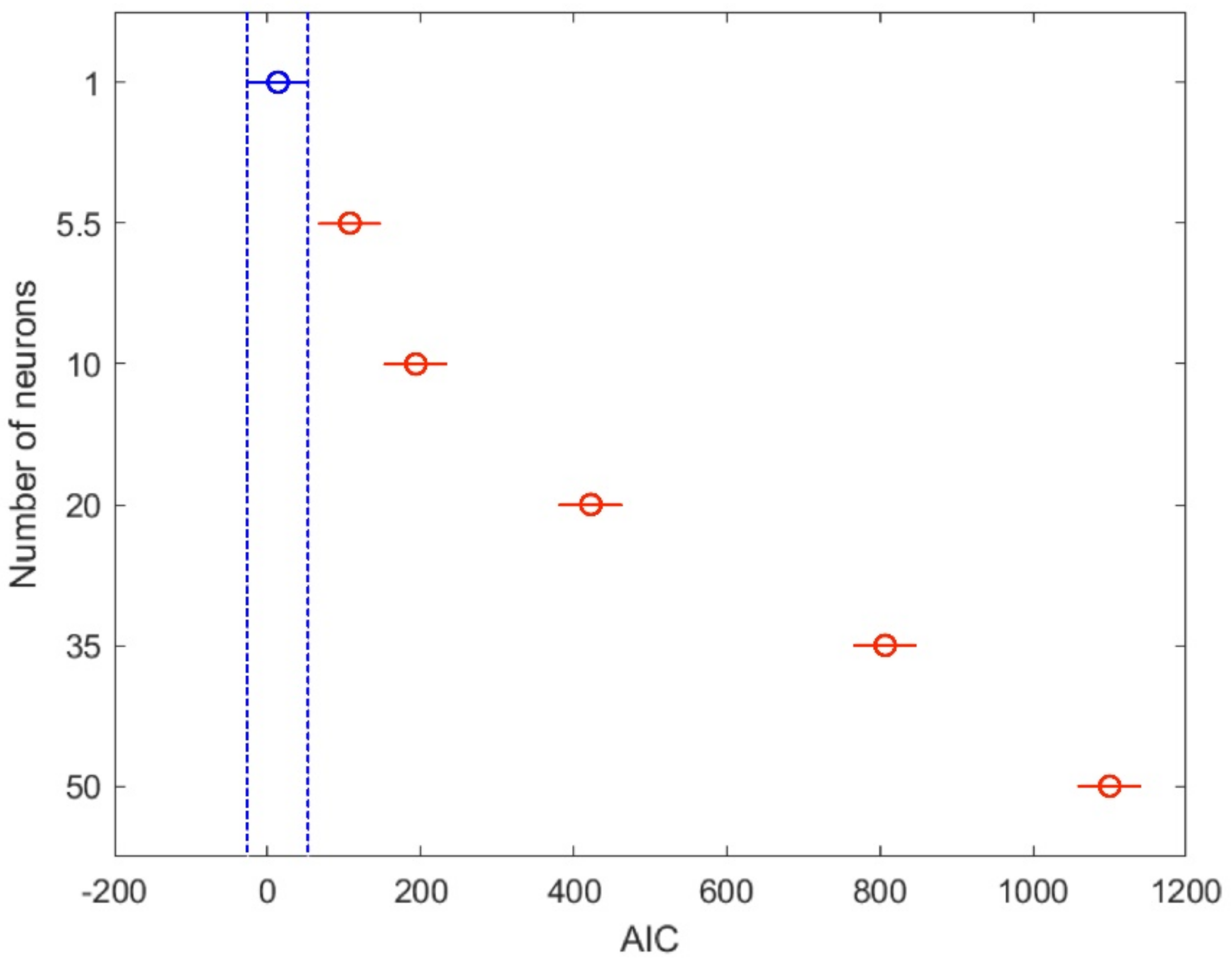
According to the regression model analysis, only the C factor is required for fitting the data to the AIC response. It is proposed to evaluate the means of observing whether there is any statistical difference between levels. The results are shown in
Table 13. In this case, we propose minimizing the AIC response with a minimum number of neurons.
Table 13 and
Table 14 show the results of LSD (Least Significant Difference) analysis. The results show that there is no statistical difference between 1 and 5.5 levels. However, the change when the number of neurons jumps to 10 is notable.
The optimal point where the system reaches a minimum AIC with a low number of neurons is less than five for one neuron in the hidden layer.
7. Forecasting Model Testing
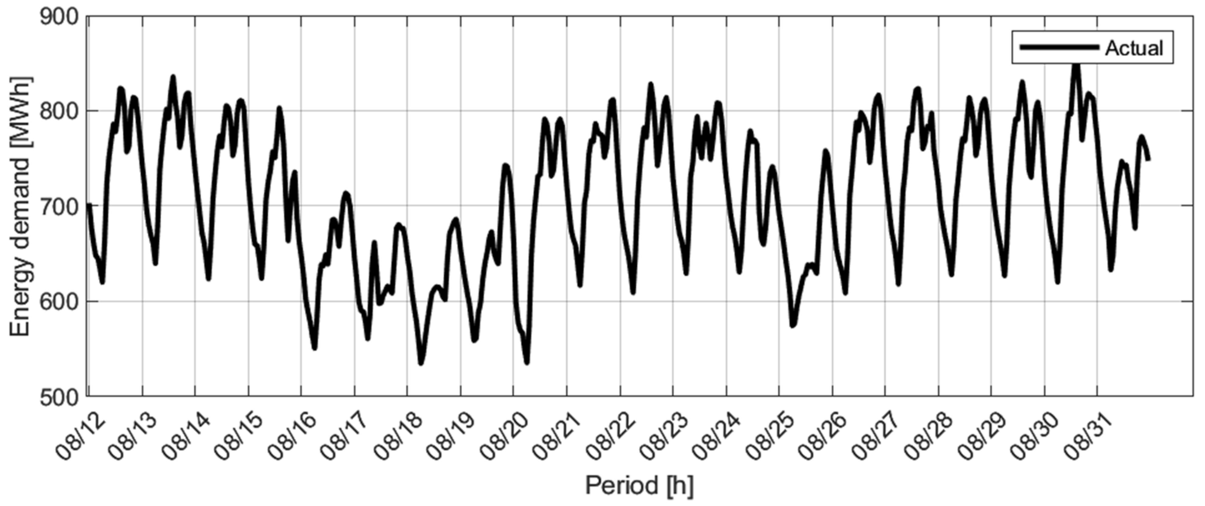
The historical energy demand data of an electricity market in Colombia (State of Atlántico) were taken in the period from 1 January 2016 to 30 September 2019 (see
Figure 4) to evaluate the performance of this proposal. Here, 70% of the data are taken for training, 15% for validation, and 15% for testing the time series. The models’ performance is validated by using one of the rolling windows with a step k that depends on the number of models for each subset. For the validation process, the separation of data into small subsets has been proposed to avoid data overlap during the training process. This ensures that the models are unaware of all the validation data. Once the model training process is done, the test data are used to evaluate the model performance. The training data selection will be made randomly and following a uniform distribution. Weather data were acquired through the website
www.accuweather.com (accessed on 30 September 2019).
Time series data of
Figure 4 are used as a reference to evaluate the results from
Section 7.
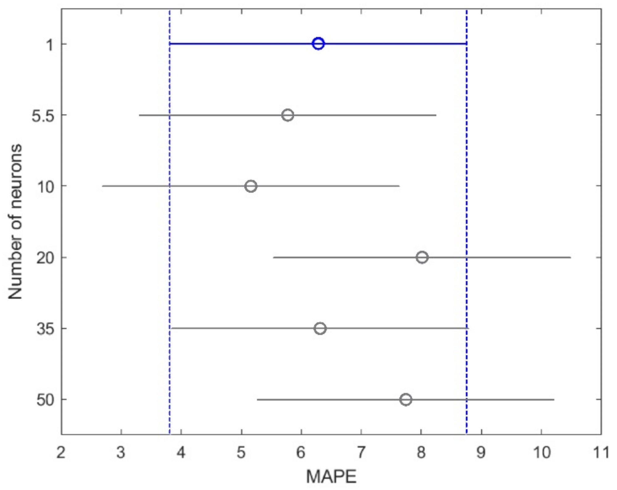
Figure 5 and
Figure 6 show that an increase in the C factor only increases the model complexity, without guaranteeing better performance in terms mainly of MAPE.
Additionally, we show how it is possible to obtain better performance by varying the number of neurons, allowing a lower computational cost due to a training process with a lower time requirement.
Table 15 shows the relationship between the number of neurons and the training time for data from the 24 periods of energy demand according to the considerations addressed in [
19].
Table 15 shows that a higher number of neurons in the training process implies an exponentially higher computational cost. Therefore, the proposed approach is key when defining an experimentation zone that reduces the time required for the training process, searching for an optimal performance value of the forecasting model.
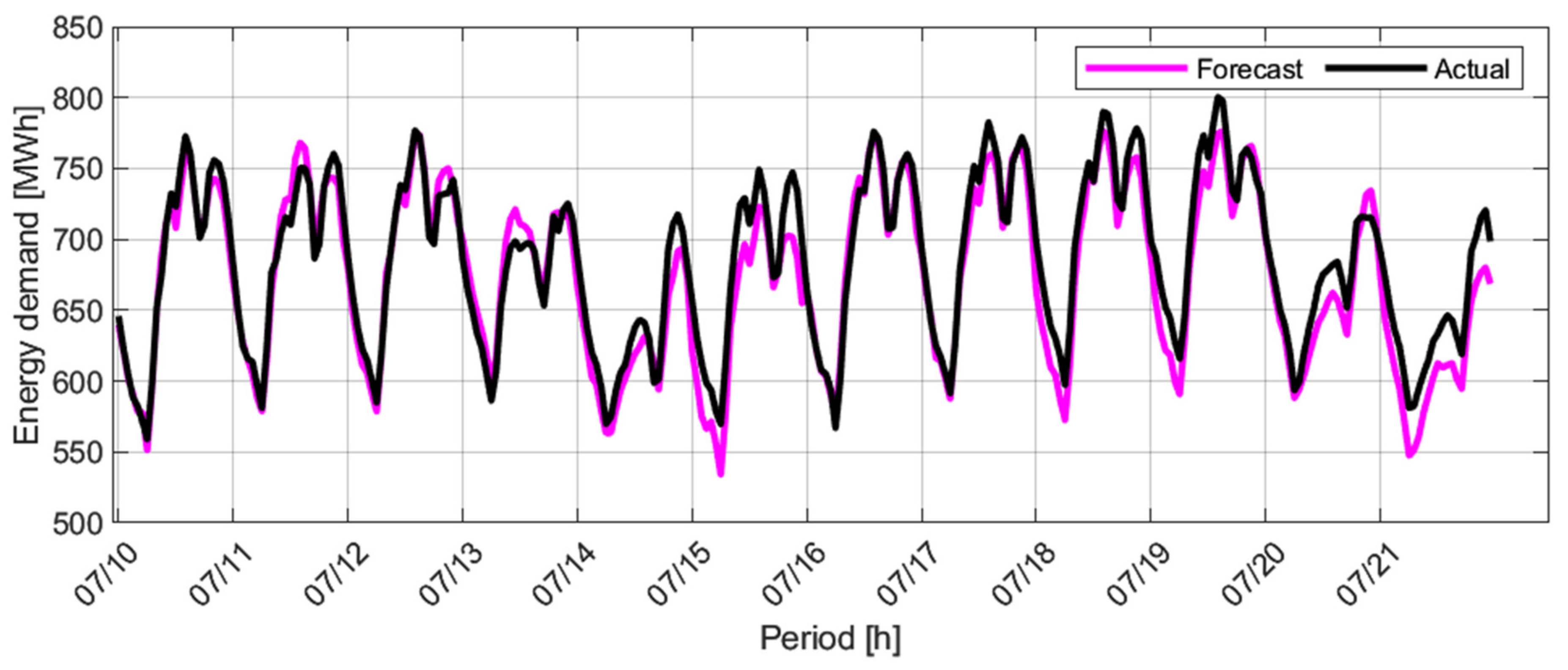
The results in the implementation of an energy demand prediction model are shown in
Figure 7, using the same methodology in the training process of the models as is used in [
16].
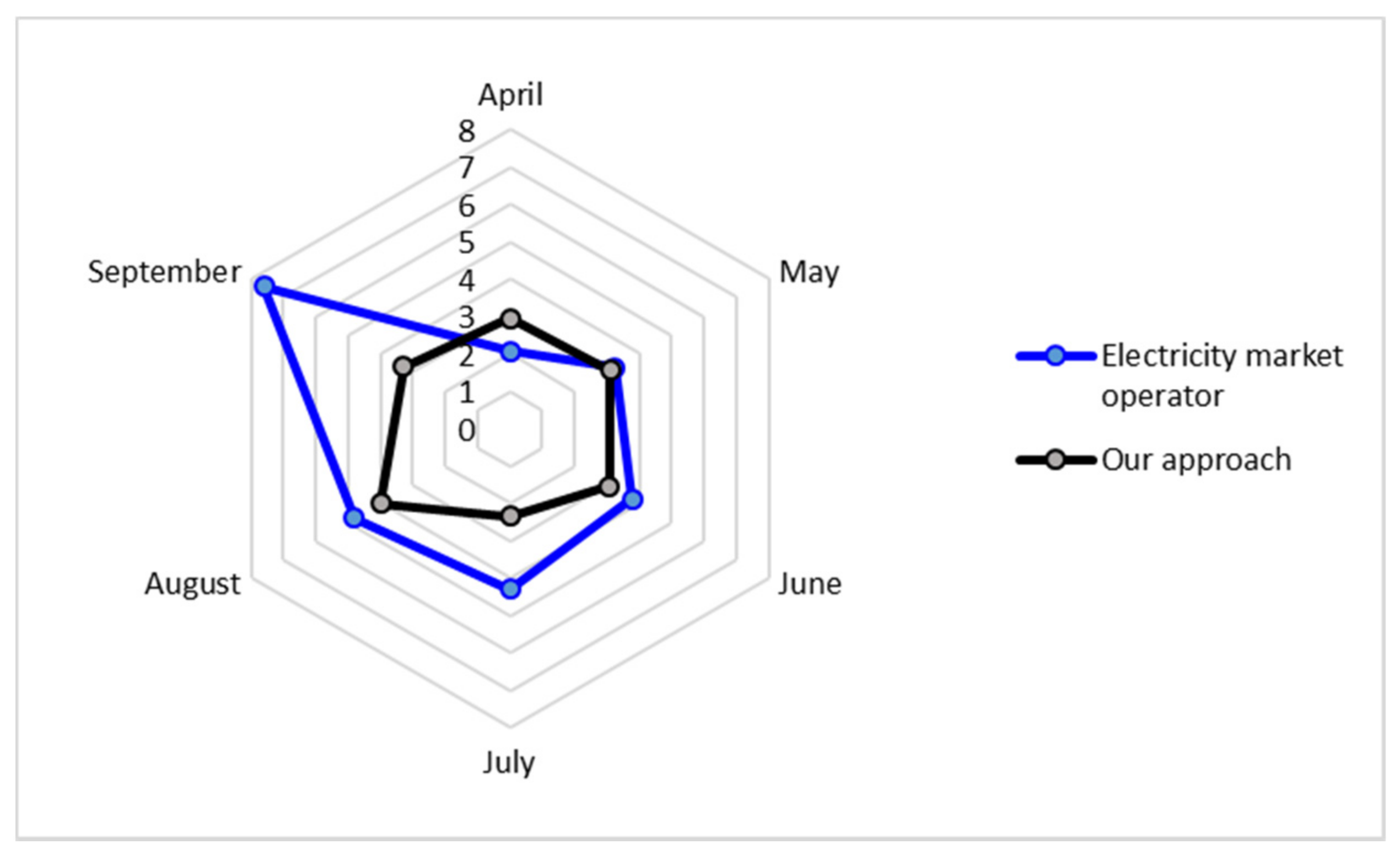
Figure 8 shows the MAPE performance of the proposed approach for the forecasting process of the Atlántico electricity market, considering the testing data from 1 April 2019 to 30 September 2019.
The forecasting models obtained through the proposed methodology evidence a better performance due to this method’s radar chart area being less than that of the Atlántico electricity market operator.
8. Conclusions
The results of this experimental design allowed us to identify that factors such as the number of hidden layers, the quantity of training data, and the validation percentage are not relevant in the network performance in terms of AIC and MAPE performance. Through the ANOVA analysis and the normal probability plot, it was possible to show initially which interaction had more relevance. In both cases, the response variable depended only on the interaction between the number of neurons and the validation percentage.
After selecting the relevant effects, a 3k design was used to detect curvature and determine the best model. In this case, only a linear model is necessary to describe the relationship between AIC and the number of neurons. There are defined as constraints a maximum of five (5) neurons and an AIC of less than 10 to optimize the regression model. An Excel solver makes it possible to find this optimal point.
Finally, multi-comparison tests showed a high difference between levels 1 and 3. A significant difference in terms of better performance was only demonstrated for a low number of neurons.
Author Contributions
Conceptualization, J.J. and C.G.Q.M.; methodology, J.J. and C.G.Q.M.; software, J.J.; validation, J.J.; formal analysis, J.J., L.N., C.G.Q.M., and M.P.; investigation, J.J., L.N., C.G.Q.M., and M.P.; resources, J.J.; data curation, J.J.; writing—original draft preparation, J.J., L.N., C.G.Q.M., and M.P.; writing—review and editing, J.J., L.N., C.G.Q.M., and M.P.; visualization, J.J.; supervision, M.P.; project administration, C.G.Q.M.; funding acquisition, J.J. and C.G.Q.M. All authors have read and agreed to the published version of the manuscript.
Funding
This research was supported by the Colombian Ministry of Science and Technology, MINCIENCIAS. Educational founding for national doctorates, Call No. 785.
Institutional Review Board Statement
Not applicable.
Informed Consent Statement
Not applicable.
Data Availability Statement
Not applicable.
Acknowledgments
This work was supported by Universidad del Norte, Barranquilla–Colombia.
Conflicts of Interest
The authors declare no conflict of interest.
References
- Orosz, T.; Rassõlkin, A.; Kallaste, A.; Arsénio, P.; Pánek, D.; Kaska, J.; Karban, P. Robust Design Optimization and Emerging Technologies for Electrical Machines: Challenges and Open Problems. Appl. Sci. 2020, 10, 6653. [Google Scholar] [CrossRef]
- Ding, Y. A novel decompose-ensemble methodology with AIC-ANN approach for crude oil forecasting. Energy 2018, 154, 328–336. [Google Scholar] [CrossRef]
- Attar, N.F.; Khalili, K.; Behmanesh, J.; Khanmohammadi, N. On the reliability of soft computing methods in the estimation of dew point temperature: The case of arid regions of Iran. Comput. Electron. Agric. 2018, 153, 334–346. [Google Scholar] [CrossRef]
- Broomhead, D.; Lowe, D. Multivariable functional interpolation and adaptive networks. Complex Syst. 1998, 2, 321–355. [Google Scholar]
- López, F.J.M.; Arriaza, J.A.T.; Puertas, S.M.; López, M.M.P. Multilevel neuronal architecture to resolve classification problems with large training sets: Parallelization of the training process. J. Comput. Sci. 2016, 16, 59–64. [Google Scholar] [CrossRef]
- Bataineh, M.; Marler, T. Neural network for regression problems with reduce training sets. Neural Netw. 2017, 95, 1–9. [Google Scholar] [CrossRef] [PubMed]
- Wang, L.; Yang, Y.; Min, R.; Chakradhar, S. Accelerating deep neural network training with inconsistent stochastic gradient descent. Neural Netw. 2017, 93, 219–229. [Google Scholar] [CrossRef] [PubMed] [Green Version]
- Lin, J.W.; Chao, C.T.; Chiou, J.S. Determining Neuronal Number in Each Hidden Layer Using Earthquake Catalogues as Training Data in Training an Embedded Back Propagation Neural Network for Predicting Earthquake Magnitude. IEEE Access 2018, 6, 52582–52597. [Google Scholar] [CrossRef]
- Li, C.H.; Yang, L.T.; Lin, M. Parallel training of an improved neural network for text categorization. Int. J. Parallel Program. 2014, 42, 505–523. [Google Scholar] [CrossRef]
- Gu, L.; Tok, D.K.S.; Yu, D.L. Development of adaptive p-step RBF network model with recursive orthogonal least squares training. Neural Comput. Appl. 2018, 29, 1445–1454. [Google Scholar] [CrossRef]
- Liang, Y.; Jiang, J.; Chen, Y.; Zhu, R.; Lu, C.; Wang, Z. Optimized Feedforward Neural Network Training for Efficient Brillouin Frequency Shift Retrieval in Fiber. IEEE Access 2019, 7, 68034–68042. [Google Scholar] [CrossRef]
- Hacibeyoglu, M.; Ibrahim, M.H. A Novel Multimean Particle Swarm Optimization Algorithm for Nonlinear Continuous Optimization: Application to Feed-Forward Neural Network Training. Sci. Program. 2018, 2018, 1435810. [Google Scholar] [CrossRef]
- Rani, R.H.J.; Victoire, T.A.A. Training Radial Basis Function Networks for Wind Speed Prediction Using PSO Enhanced Differential Search Optimizer. PLoS ONE 2018, 13, e0196871. [Google Scholar] [CrossRef] [PubMed] [Green Version]
- Chouikhi, N.; Alimi, A.M. Adaptive Extreme Learning Machine for Recurrent Beta-basis Function Neural Network Training. arXiv 2018, arXiv:1810.13135. [Google Scholar]
- Jimenez, J.; Pertuz, A.; Quintero, C.; Montana, J. Multivariate statistical analysis based methodology for long-term demand forecasting. IEEE Lat. Am. Trans. 2019, 17, 93–101. [Google Scholar] [CrossRef]
- Mares, J.J.; Navarro, L.; Quintero, M.C.G.; Pardo, M. A methodology for energy load profile forecasting based on intelligent clustering and smoothing techniques. Energies 2020, 13, 4040. [Google Scholar] [CrossRef]
- Zhang, Q.J.; Gupta, K.C. Neural Networks for RF and Microwave Design, 1st ed.; Artech House: Norwood, MA, USA, 2000. [Google Scholar]
- Montgomery, D. Diseño y Análisis de Experimentos, 2nd ed.; Wiley, Limusa: Mexico City, Mexico, 2005. [Google Scholar]
- Jiménez, J.; Donado, K.; Quintero, C.G. A Methodology for Short-Term Load Forecasting. IEEE Lat. Am. Trans. 2017, 15, 400–407. [Google Scholar] [CrossRef]
Figure 1.
Normal probability plot for Akaike information criterion (AIC).
Figure 1.
Normal probability plot for Akaike information criterion (AIC).
Figure 2.
Normal probability plot for Mean Absolute Percentage Error (MAPE).
Figure 2.
Normal probability plot for Mean Absolute Percentage Error (MAPE).
Figure 3.
Residuals for the C factor.
Figure 3.
Residuals for the C factor.
Figure 4.
Actual data for the energy demand of Atlántico electricity market.
Figure 4.
Actual data for the energy demand of Atlántico electricity market.
Figure 5.
Multi-comparison test: AIC vs. number of neurons.
Figure 5.
Multi-comparison test: AIC vs. number of neurons.
Figure 6.
Multi-comparison test: MAPE vs. number of neurons.
Figure 6.
Multi-comparison test: MAPE vs. number of neurons.
Figure 7.
Forecast and actual data for the energy demand of the Atlántico electricity market.
Figure 7.
Forecast and actual data for the energy demand of the Atlántico electricity market.
Figure 8.
Performance comparison of the model used by the Atlántico electricity market operator and the proposed approach.
Figure 8.
Performance comparison of the model used by the Atlántico electricity market operator and the proposed approach.
Table 1.
Summary of techniques commonly used in the training of time series models.
Table 1.
Summary of techniques commonly used in the training of time series models.
| Author | Training Techniques |
|---|
| ANN | RBF | OLS | BPNN | FFN | SGD |
|---|
| [5] | ✓ | ✓ | | | | |
| [6] | ✓ | | ✓ | | ✓ | |
| [7] | ✓ | | | | | ✓ |
| [8] | | | | ✓ | | |
| [9] | ✓ | | | ✓ | | |
| [10] | ✓ | ✓ | | | | |
| [11] | ✓ | | | | ✓ | |
| [12] | ✓ | | | | ✓ | |
| [13] | ✓ | ✓ | | | | |
| [14] | | ✓ | ✓ | | ✓ | |
| [15] | | | | | ✓ | |
Table 2.
Factors design.
| Factors | Levels |
|---|
| Low | High |
|---|
| Training algorithm | Levenberg–Marquardt | Resilient Backpropagation |
| Number of hidden layers | 1 | 5 |
| Number of neurons in the hidden layer | 1 | 10 |
| Data number | 60 | 120 |
| Validation percentage | 10 | 30 |
Table 4.
Normality test for AIC.
Table 4.
Normality test for AIC.
| Test | p-Value |
|---|
| Chi-square | 0.1319 |
Table 5.
Homoscedasticity test for AIC.
Table 5.
Homoscedasticity test for AIC.
| | Levene′s Test | p-Value |
|---|
| B | 1.38557 | 0.263 |
| C | 1.54509 | 0.22749 |
| D | 1.61809 | 0.2127 |
| E | 1.73115 | 0.1919 |
Table 6.
ANOVA for MAPE.
| Source | Sum of Squares | Degrees of Freedom | Mean Square | F-Ratio | p-Value |
|---|
| A: Train_Alg | 0.871079 | 1 | 0.871079 | 2.78 | 0.1096 |
| B: Hidd_Num | 0.0182764 | 1 | 0.0182764 | 0.06 | 0.8114 |
| C: Neu_Num | 0.0201734 | 1 | 0.0201734 | 0.06 | 0.8020 |
| D: Data_Num | 0.00900434 | 1 | 0.00900434 | 0.03 | 0.8669 |
| E: Val_Per | 0.331972 | 1 | 0.331972 | 1.06 | 0.3145 |
| AB | 0.0507545 | 1 | 0.0507545 | 0.16 | 0.6912 |
| AC | 0.00168203 | 1 | 0.00168203 | 0.01 | 0.9422 |
| AD | 0.0519588 | 1 | 0.0519588 | 0.17 | 0.6877 |
| AE | 0.446753 | 1 | 0.446753 | 1.43 | 0.2451 |
| BC | 0.567389 | 1 | 0.567389 | 1.81 | 0.1921 |
| BD | 0.0440187 | 1 | 0.0440187 | 0.14 | 0.7114 |
| BE | 0.412097 | 1 | 0.412097 | 1.32 | 0.2637 |
| CD | 0.048383 | 1 | 0.048383 | 0.15 | 0.6981 |
| CE | 1.75907 | 1 | 1.75907 | 5.62 | 0.0270 |
| DE | 0.00784171 | 1 | 0.00784171 | 0.03 | 0.8757 |
| Error total | 6.89167 | 22 | 0.313258 | | |
| Total (corrected error) | 11.5321 | 37 | | | |
Table 7.
Normality test for MAPE.
Table 7.
Normality test for MAPE.
| Test | p-Value |
|---|
| Chi-square | 0.0269 |
Table 8.
Homoscedasticity test for MAPE.
Table 8.
Homoscedasticity test for MAPE.
| Factor | Levene′s Test | p-Value |
|---|
| B | 0.327 | 0.722 |
| C | 0.305 | 0.738 |
| D | 0.366 | 0.685 |
| E | 0.876 | 0.425 |
Table 9.
Levels of model analysis.
Table 9.
Levels of model analysis.
| Neu_Num (C) | Val_Per (E) | AIC |
|---|
| 1 | 10 | 18.2656065 |
| 5.5 | 20 | 2.35135344 |
| 10 | 20 | 165.831393 |
| 5.5 | 10 | 53.4919072 |
| 1 | 20 | 7.9016126 |
| 10 | 10 | 200.675933 |
| 1 | 10 | 19.8895334 |
| 5.5 | 20 | 105.424653 |
| 10 | 20 | 175.661213 |
| 5.5 | 10 | 121.928836 |
| 1 | 20 | 29.8195033 |
| 10 | 10 | 159.069137 |
Table 10.
Coefficients test.
Table 10.
Coefficients test.
| | Coefficient | Typical Error | t-Statistic | p-Value |
|---|
| Number of neurons | 16.46 | 1.44 | 11.38 | 1.9 × 10⁻⁷ |
Table 11.
Grouped regression statistics of the model analysis.
Table 11.
Grouped regression statistics of the model analysis.
| Regression Statistics |
|---|
| R_pearson | 0.96010775 |
| R2 | 0.92180688 |
| Adjusted R2 | 0.83089779 |
| Typical error | 33.1356306 |
| Observations | 12 |
Table 12.
ANOVA for model analysis.
Table 12.
ANOVA for model analysis.
| Source | Degrees of Freedom | Sum of Squares | Mean Square | F-Ratio | p-Value |
|---|
| Regression | 1 | 142,381.8 | 142,381.8 | 129.677347 | 4.7736 × 10⁻⁷ |
| Residues | 11 | 12,077.6 | 1097.97 | | |
| Total | 12 | 154,459.5 | | | |
Table 13.
ANOVA for C Factor (number of neurons).
Table 13.
ANOVA for C Factor (number of neurons).
| Source | Sum of Squares | Degrees of Freedom | Mean Square | F-Ratio | p-Value |
|---|
| Between groups | 50,734.7 | 2 | 25,367.4 | 22.75 | 0.0003 |
| Within groups | 10,036.5 | 9 | 1115.17 | | |
| Total (corrected error) | 60,771.3 | 11 | | | |
Table 14.
Fisher LSD test.
Table 14.
Fisher LSD test.
| Neu_Number | Cases | Mean | Homogenous Group |
|---|
| 1 | 4 | 18.9691 | X |
| 5.5 | 4 | 70.7992 | X |
| 10 | 4 | 175.309 | X |
Table 15.
Relationship between number of neurons and training time.
Table 15.
Relationship between number of neurons and training time.
| Number of Neurons | Training Sime (s) |
|---|
| 1 | 0.285186 |
| 10 | 0.284743 |
| 20 | 0.466448 |
| 50 | 7.847768 |
| Publisher’s Note: MDPI stays neutral with regard to jurisdictional claims in published maps and institutional affiliations. |
© 2021 by the authors. Licensee MDPI, Basel, Switzerland. This article is an open access article distributed under the terms and conditions of the Creative Commons Attribution (CC BY) license (https://creativecommons.org/licenses/by/4.0/).


