CFD Analysis and Shape Optimization of Airfoils Using Class Shape Transformation and Genetic Algorithm—Part I

Abstract

This paper presents the parameterization and optimization of two well-known airfoils. The aerodynamic shape optimization investigation includes the subsonic (NREL S-821) and transonic airfoils (RAE-2822). The class shape transformation is employed for parametrization while the genetic algorithm is used for optimization purposes. The absolute scheme of the optimization process is carried out for the minimization of the drag coefficient and maximization of lift to drag ratio. In-house MATLAB code is incorporated with a genetic algorithm to calculate the drag coefficient and lift to drag ratio of the resulting optimized airfoil. The panel method is utilized in genetic algorithm optimization code to calculate pressure distribution, lift coefficient, and lift to drag ratio for optimized airfoil shapes and validates with XFOIL and NREL experimental data. Furthermore, CFD analysis is conducted for both the original (NREL S-821) and optimized airfoil obtained. The present method shows that the optimized airfoil achieved an improvement in lift to drag ratio by 7.4% and 15.9% of S-821 and RAE-2822 airfoil, respectively, by the panel technique method and provides high design desirable stability parameters. These features significantly improve the overall aerodynamic performance of the newly optimized airfoils. Finally, the improved aerodynamics results are reported for the design of turbulence modeling and NREL phase II, Phase III, and Phase VI HAWT blades.

1. Introduction

The increase in global energy consumption and the decrease in fossil fuels forces governments to spend more on alternative energy resources. Wind energy is alternative renewable energy that is clean, economical, and available in abundant quantity [1,2]. The fast-growing trend of wind energy worldwide has increased the demand for efficient and optimized performance of airfoil, which further paved the way for energy harvesting systems. To harvest maximum energy from the wind, a properly designed airfoil is required for wind turbine blades to maximize lift and minimize drag. Therefore overall researches need to be improved to meet essential needs for the aerodynamic performance of wind turbines. Airfoil design is important to increase the aerodynamic performance of a wind turbine rotor. The selection of an optimum aerodynamic design that effectively fits a specified range of flow conditions is very important. Nowadays, the optimization of aerodynamic shape has become crucial with the rapid development of aerospace and mechanical engineering. As Igor Rodriguez-Eguia et al. [3] explained, the idea to control devices and aerodynamic shapes that locally change the aerodynamic performance of the airfoil on the wind turbine blade. The parametric method in aerodynamic shape plays a crucial role in the optimized process of airfoil optimization. A good parameterization method with fewer design parameters can handle larger shape changes of the wing in the design space [4].

Due to the industrial revolution and new computational fluid dynamics and technological changes, some numerical tools for optimizing airfoils have been developed instead of using plate theory to design airfoils [5]. Two main approaches for the design of aerodynamic shapes are (a) Inverse design (ID) and (b) Direct Numerical Optimization (DNO) [6,7]. The first method solves the geometry and searches for different airfoils that can meet the demand of fluid dynamic structure and as a result, it produces pressure distribution. The second method (DNO) combines with geometric definition and analysis is done for aerodynamic shape in an iterative process to generate the best concerning different goals and constraints. The above methods indicate that it is necessary to modify the present airfoil design or to achieve a new and better design through partial airfoil modification by applying even different parameterization methods. These local airfoil shape modifications can be achieved through analytical function by smooth perturbations of original airfoil coordinates, for instance, Bernstein polynomials [8]. ASO is a combination of parameterization and optimization process as well as design analysis of aerodynamic shape. The parameterization method has a great impact on the optimization output which can accommodate a large number of potential airfoils with smaller design variables in design space [9]. In a recent study, Nili et al. developed and employed an inverse design method and linked it with Ball Spine Algorithm (BSA), which showed promising results to solve complex geometries for various flow regimes [10,11]. Different parameterization techniques have been developed to parameterize the aerodynamic shape [12]. A variety of parametric methods which are implemented to ASO are the PARSEC method, B-spline, Bezier curves which are used to fit aerodynamic shapes by interpolation methods [13,14]. Hicks–Henne’s [15] function was explained earlier in their work about airfoil families which can be represented by deriving analytical functions. The result of these above methods cannot be used to design new concepts but the methods are robust enough to illustrate different airfoils. Due to the larger number of parameters used in the airfoil, the search for optimized design results is more feasible [15,16,17,18]. However, due to an increase in design variable which leads to increase inevitably, the search problem of optimization algorithms are not beneficial to search-optimized design results. Optimization of an airfoil plays another important role where aerodynamic performance is optimized to obtain benefits in drag minimization or high endurance if the L/D ratio is maximized. The shape of the airfoil changes by optimization process to achieve the objective function, but it is too compact to use all of the design variable sets during the optimization process. Therefore, the variables used for design should be reduced from almost infinite to a limited set, and a parametric method should be used to illustrate a new airfoil or initial airfoil. Samareh [19] has surveyed parameterization techniques and confirmed that the method has a great impact on the optimization process in aerodynamic shape design. Ulaganathan and Balu [20] believe that polynomial methods based on parameterization will strongly influence the design variables generated through an optimization process.

Some physically tried and tested methods allowed us to use the parameters of the airfoil to define its shapes, such as angle of the trailing edge, wing thickness, and radius of the leading-edge. Kulfan and Bussoletti [21,22,23] introduced a new parametrization technique which is also called Kulfan parameters, or CST method. This CST parameterization is a powerful method because of its simplicity and robustness. Sobieczky [24] presented a new methodology for parameterization called PARSEC. A total of 11 parameters are used to define the shape of the airfoil. It has designed a variety of aerodynamic shapes with smooth geometric shapes, with fewer parameters and equations [25]. With a lower order polynomial, preliminary design and optimization of the airfoil can be easy since only a few numbers of parameters are required to control the shape of an airfoil. Since the CST equation is an addition operation of the Bezier curve with a class function term so CST is considered to be very similar to the Bezier curve. Different aerodynamic shapes are derived from the class function which is classified as basic functions. These aerodynamic shapes are biconvex, Sears–Haack body, round nose, and pointed aft end airfoil which is similar to NACA airfoil, oval airfoil, wedge airfoil, and some other different airfoils. These types of airfoils can be converted into axisymmetric bodies, can also be modified by shape function to obtain a new airfoil shape. The shape function in the same class is indicated by the class function has its geometric shape. Compared with the Bezier curve, the advantage of CST is that it can fit the curve to specific shapes with a smaller coefficient.

Related to the previous literature, in this study the CST parametrization in combination with a genetic algorithm has been employed to bring forward a unified solution for aerodynamic shape optimization. The prime motive is carrying out the optimized shapes in a simplified manner by considering airfoil shapes as under-investigated profiles. The subsonic NREL S-821 airfoil and transonic RAE-2822 airfoil are selected for this purpose, which is the most commonly used for aerospace and wind energy applications. The panel method technique is used to calculate the drag coefficient of the airfoil. The resulting lift to drag ratio of the optimized and baseline airfoil are correlated with the NREL experimental data to verify the proposed optimization method. Besides, numerical validation and CFD analysis were implemented for the S-821 airfoil to check the applicability of the airfoil constraint inside the structured mesh in the numerical simulation and compared it with the experimental results. Findings are described in detail and shown with indicators like pressure coefficient, convergence graph, and grid independence study. Finally, the coefficient of drag (Cd), lift coefficient (Cl) and lift to drag (L/D) ratio for baseline and optimized airfoil at 3° angle of attack (AOA) is discussed and reported in the paper. The shape optimization of the baseline airfoil used in the paper has a great impact on the energy harvesting system of the wind turbine blades. Nevertheless, the expected results based on the CFD-derived data can be slightly proved that the novelty of the research method is a better technique that can be easily applied in the energy field.

2. Mathematical Model

2.1. CST Parametrization of Airfoil

CST is an effective parameterization technique and relatively powerful as well for modeling two-dimensional and three-dimensional aerodynamic shapes using Bernstein polynomials. The CST method is not limited to the shape of the airfoil and can also produce other aerodynamic shapes. Equations (1) and (2) are the coefficients of two arrays which are designed to show the CST method which differentiates the airfoils from one another. The curvature coefficients of the lower and upper surfaces of the airfoil are controlled by the coefficient of CST arrays [26]. These curvature coefficients further provide a set of design variables that are utilized in the optimization of the airfoil shape. This parametric scheme covers a wide range of airfoils, making it equally suitable for any shape of airfoils. Later in the paper, it is described mathematically that CST consists of two main elements, namely the shape function and the class function. The class function of the airfoil handles the fixed parameters inside the class function itself. For CST and Bernstein Polynomial the smoothness of the curve plays a crucial role for optimization purposes. CST is explained mathematically in the coming paragraph.

Equations (1) and (2) shows the relation between the upper and lower surface of CST, where ‘C’ = class function and ‘S’ = shape function. The upper and lower surfaces are expressed as follows:

$${\left(\frac{y}{c}\right)}_{upper}=C_{N_2}^{N_1}\left(\frac{x}{c}\right)S_U\left(\frac{x}{c}\right)+\frac{x}{c} \frac{z_{u,TE}}{c}$$

(1)

$${\left(\frac{y}{c}\right)}_{lower}=C_{N_2}^{N_1}\left(\frac{x}{c}\right)S_L\left(\frac{x}{c}\right)+\frac{x}{c} \frac{z_{l,TE}}{c}$$

(2)

where, $z_{u,TE}$ and $z_{l,TE}$ are trailing edge thickness of upper and lower surface, respectively. $N_1=0.5$ and $N_2=1$ is constant. The class function draws the main contours of the aerodynamic shape, while the shape function creates a fixed shape within the same geometric category. The class function can be expressed by the following equation

$$C_{N_2}^{N_1}\left(\frac{x}{c}\right)={\left(\frac{x}{c}\right)}^{N_1}{\left(1-\frac{x}{c}\right)}^{N_2}$$

(3)

The CST parameterization method airfoils are derived from class function. The exponent $N_1$ and $N_2$ are replaced by the values 0.5 and 1.0, respectively to represent the upper and lower surface of an airfoil [26]. To show an airfoil, Equations (1) and (2) can be written as:

$${\left(\frac{y}{c}\right)}_{upper}=C_{1.0}^{0.5}\left(\frac{x}{c}\right)S_U\left(\frac{x}{c}\right)+\frac{x}{c} \frac{z_{u,TE}}{c}$$

(4)

$${\left(\frac{y}{c}\right)}_{lower}=C_{1.0}^{0.5}\left(\frac{x}{c}\right)S_L\left(\frac{x}{c}\right)+\frac{x}{c} \frac{z_{l,TE}}{c}$$

(5)

The general shape function for $S_U$ (for upper surface) and $S_L$ (for lower surface) defines specific shapes within the same class of airfoil as shown in Equations (6) and (7):

$$S_U\left(\frac{x}{c}\right)={\displaystyle \sum }_{i=0}^{N_U}{W}_U\left(i\right) S\left(\frac{x}{c},i\right)$$

(6)

$$S_L\left(\frac{x}{c}\right)={\displaystyle \sum }_{i=0}^{N_L}{W}_L\left(i\right) S\left(\frac{x}{c},i\right)$$

(7)

where $W_U$ = upper surface weights and $W_L$ = lower surface weights, $N_U$ and $N_L$ denote the number of shape functions for the upper and lower surface, respectively. S is a component shape function that is different for the upper and lower surface. The equation of component shape function is shown below:

$$S\left(\frac{x}{c}, i\right)=K_i^N\ast S\left(\frac{x}{c}\right){ }^i\ast {\left(1-\frac{x}{c}\right)}^{N-i}$$

(8)

where $K$ denotes Binomial coefficient which belongs to order N Bernstein polynomial as follows:

$$K_i^N=\frac{N!}{i!\left(N-i\right)!}$$

(9)

The above Equations (3)–(9) are solved to produce a complete form of equations for both surfaces of airfoils are expressed in Equations (10) and (11) as follows:

$${\left(\frac{y}{c}\right)}_{upper}= {\left(\frac{x}{c}\right)}^{0.5}\ast \left(1-\frac{x}{c}\right) {}^{1.0} {\displaystyle \sum }_{i=0}^{N_U}\left[W_U\left(i\right)\ast \frac{N_U!}{i!\left(N_U-i\right)!}\ast {\left(\frac{x}{c}\right)}^i\left(1-\frac{x}{c}\right) {}^{N_U-i}\right]+\frac{x}{c} \frac{z{u}_{TE}}{c}$$

(10)

$${\left(\frac{y}{c}\right)}_{lower}= {\left(\frac{x}{c}\right)}^{0.5}\ast \left(1-\frac{x}{c}\right) {}^{1.0} {\displaystyle \sum }_{i=0}^{N_L}\left[W_L\left(i\right)\ast \frac{N_L!}{i!\left(N_L-i\right)!}\ast {\left(\frac{x}{c}\right)}^i\left(1-\frac{x}{c}\right) {}^{N_L-i}\right]+\frac{x}{c} \frac{z{l}_{TE}}{c}$$

(11)

The Equations (10) and (11) provide perfect curvature coefficients to an airfoil. Further curvature coefficients are optimized to generate an airfoil profile and a new set of design variables is obtained from parametrization by the CST method. Figure 1 presents an airfoil generated by CST parameterization using 2nd order Bernstein polynomial, where $N_1$ and $N_2$ is kept 0.5 and 1.0, respectively [27]. In Figure 1, the base airfoil shows the initial airfoil in red, and the blue dot line represents airfoil generated by CST parametrization.

2.2. Optimization Scheme

At present for challenging engineering problems, there are different numerical design techniques to achieve solutions. Since there are several optimization algorithms in the literature, it is very important to choose a suitable search algorithm for aerodynamic shape optimization. Here genetic algorithm (GA) is selected for the optimization process. To get an optimized result of both the airfoil NREL S-821 and RAE-2822, GA and flow solver XFOIL were linked with in-house MATLAB code to obtain the coefficients of an airfoil. These coefficients are generated with the help of design variables obtained from the CST method during the parametrization process. These design variables are used in the optimization process as the main task. As per the previous study, optimization problems are of two types, Constrained and unconstrained. These optimization problems based on the principle of natural selection are solved by a genetic algorithm. The process of GA drives biological evolution and is used to optimize the shape of the airfoil. The process of optimization for each scenario was performed with a default population size (Ps) of 50 and the maximum generation of 200. The conditions employed for aerodynamic flow parameters in the optimization process include Re, Ma, and AOA. The single-objective function for the optimization of an airfoil is expressed as:

$$\mathrm{Minimize}:f\left(x\right)=Cd$$

(12)

The main goal is to attain the maximum value of aerodynamic performance by minimizing Cd and maximizing the L/D ratio. For aerodynamic shape optimization, GA is used in a large design space. The probabilities of operating crossover and mutation on each generation are 0.5 and 0.01, respectively. The optimized airfoil profile of NREL S-821 and RAE-2822 are shown in Figure 2.

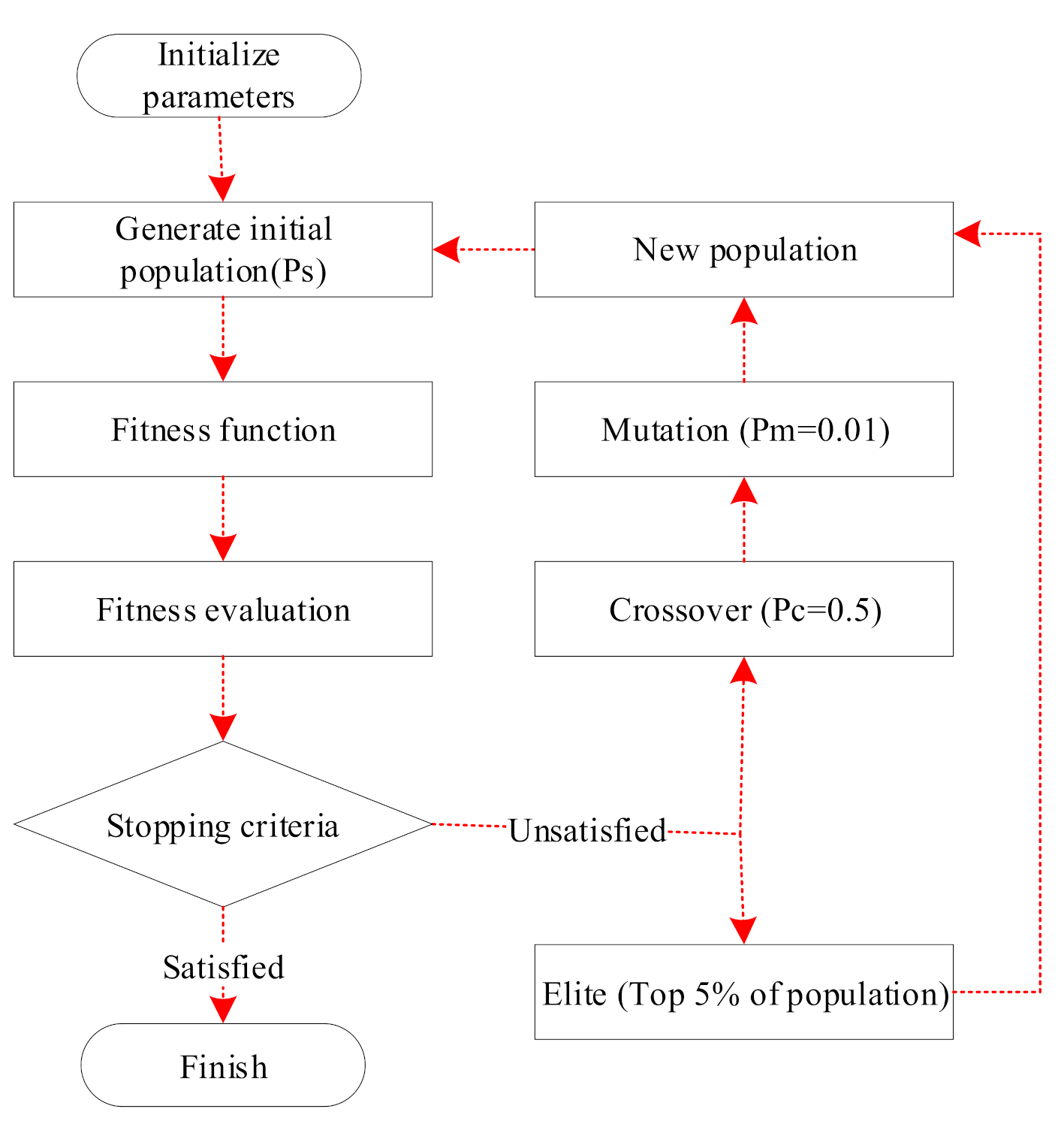
2.3. Genetic Algorithm

Genetic algorithm (GA) is also known as evolutionary algorithm based on natural selection process contrary to gradient optimization technique. A genetic algorithm was introduced by John Holland in 1960 based on Darwin’s theory of evolution and later it was carried out further by David Goldberg [28] in 1989. GA is a metaheuristic technique, motivated by Charles Darwin’s theory of natural evolution which relates to the bigger class of evolutionary algorithm (EA). The concept of GA is applied to optimization problems to obtain optimal solutions. The whole process of evolution was carried out through bio-inspired operators such as crossover, mutation, and selection [29]. For the solution process, each chromosome was ranked accordingly to its fitness vector. For each objective, one fitness value was allotted. The values with the highest-ranking continue to next-generation while the low-value ranking of chromosomes has a very less probability of selection. A new set of artificial strings are generated by using the fragments of the most suitable value in each generation, and this new part is used for good measure. The chromosomes which are newly selected are manipulated in the next generation using operators such as selection, mutation, and crossover to generate a final set of chromosomes for the new generation. The process of iterating continues from generation to generation until the algorithm terminates and it happens when the suitable level of convergence is obtained or the maximum number of generations has been produced. It works theoretically well in the non-smooth design spaces. This method is also good for the multi-objective optimization process and computes Pareto optimal sets in place of the limited single point design optimization. The basic GA flow chart which has been adopted during developing MATLAB code is explained in Figure 3.

2.3.1. Initialization

The initial population generates optimized parameters randomly between 0 and 1 and allows all the possible ranges for the solution. The bit value is fixed, depends on the range of random numbers. For a number between 0–0.5 and 0.5–1, the bit will be taken as 0 and 1, respectively. Population size (Ps) controls the size of the initial population and it can be determined by the nature of the problem which contains several hundred or thousands of possible solutions. Population size must be even in number.

2.3.2. Selection

Selection’s role is to select the best solution and let them pass their genes to the next generation. These fittest individuals are further coupled and generate new offsprings. The individuals with desirable properties are selected in the next generation which is adapted by the tournament wheel selection process which is determined by a particular selection process among the individuals. The individuals with the highest fitness value will be considered the winner of the tournament and placed in the mating pool. The selection process has some important properties: (i) best fit individuals are favored but not chosen always, (ii) individuals with worst fitness value are not always eliminated to maintain the variability in generation.

2.3.3. Crossover

Crossover is a genetic operator used to combine the genetic information of two parents to generate new offspring. This depends on the method of encoding and the types of problems to be solved. Crossover facilitates the algorithm to remove the best genes from different individuals which are then recombined into a potentially superior one. Various approaches are available for a crossover but a uniform crossover approach is employed in this paper. The current research includes crossover probability (Pc = 0.5) and a probability test is performed for each bit in the bit string. These bits are randomly exchanged between the two parents who choose to pair and it continues until it reaches the crossover point. Figure 4 explains the formation of offspring from parents by exchanging their genes.

2.3.4. Mutation

The main role of the mutation is to alter one or more gene values in a chromosome from its initial state. As a result, the solution is changed entirely from the previous one and gives a better solution. Here mutation probability (Pm = 0.01) is defined and the test is performed in the bit string on each bit. If the test is passed, the bits in the bit string are flipped and compared with the original one. Mutation probability cannot be less than equal to zero and greater than equal to 1. The probability of mutation can be described by relation as shown in Equation (13).

$$\mathrm{Pm}= \frac{\sum \left(bits\right)+1}{2\ast P_s\ast \sum \left(bits\right)}$$

(13)

2.3.5. Fitness Evaluation

The procedure of objective function evaluation for each set of optimized parameters is labeled as fitness evaluation. After the fitness of the new offsprings, they become new parents and are chosen for further mating. The process is continued until the convergence is attained. Fitness function must not correlate with the designer’s goal but also it must compute the problem quickly.

2.3.6. XFOIL

XFOIL is a flow solver for the analysis and design of isolated airfoils. Furthermore, the optimization algorithm combines with an XFOIL in a single script MATLAB code [30]. The airfoil coordinates are provided to XFOIL through MATLAB program after the optimization process by GA. The shape of the 2D airfoil is specified using these coordinates. Through the panel technique method, i.e., XFOIL, the pressure distribution, lift and drag characteristics of the airfoil are calculated. It takes input as the coordinates of an airfoil, Reynolds number, and Mach numbers to generate the required results.

The whole transformation and optimization schemes start with the selection of airfoils, parametrization method, and an optimization algorithm. As it has been described earlier in the manuscript that instead of designing new airfoils, the existing well-known with common application airfoils NREL S-821 and RAE-2822 were selected for this study. CST parameterization and GA for optimization of an airfoil in the design phase is the most important part. Hence, in this paper, the shape parameterization by CST method is implemented for subsonic (NREL S-821) and transonic airfoils (RAE-2822) in the MATLAB environment. Further CST method is linked with GA in-house MATLAB code for optimization purposes.

3. Methodology

The whole transformation and optimization schemes start with the selection of airfoils, parametrization method, and an optimization algorithm. As has been described earlier in the manuscript, instead of designing new airfoils, the existing well-known with common application airfoils NREL S-821 and RAE-2822 were selected for this study. CST parameterization method and GA for optimization of an airfoil in the design phase are implemented for subsonic (NREL S-821) and transonic airfoils (RAE-2822) in MATLAB environment. Further CST code is linked with GA code in MATLAB for the optimization process. XFOIL based flow solver is called in the GA optimization process to calculate Cd, Cl, and L/D ratio for generated optimized airfoil, and pressure distribution curve is extracted at 3° AOA. Finally, on the other hand, CFD analysis on ANSYS CFX using the structured mesh was also performed for NREL S-821 for both the original and optimized airfoil generated by the optimization process. The complete analysis procedure is organized and shown in Figure 5, as a flowchart

3.1. Computational Model

As additional validation of the resulted airfoil, a computational study conceded out by solving a compressible form of Reynolds Averaged Navier–Stokes equation (RANS) and continuity equation. The mass and momentum conservation equations are expressed as follows [31,32,33]:

$$\frac{\partial }{\partial x_i}\left(\rho u_i\right)=0$$

(14)

$$\frac{\partial \left(\rho u_i{u}_j\right)}{\partial x_j}=\frac{\partial p}{\partial x_i}+\frac{\partial }{\partial x_i}\left(\mu \left(\frac{\partial u_i}{\partial x_j}+\frac{\partial u_j}{\partial x_i}-\frac{2}{3}{\delta }_{ij}\frac{\partial u_j}{\partial x_i}\right)\right)+\frac{\partial }{\partial x_j}\left(-\rho \overline{{\acute{u}}_i{\acute{u}}_j}\right)+\rho f_b$$

(15)

where $\rho$ = density, $p$ = pressure, $\mu$ = dynamic viscosity and $f_b$ denotes body forces. $u_i$ and $u_j$ denotes velocity vectors for $i, j=1,2,3$. Another unknown term in Equation (15) are Reynold stresses, i.e., $\left(\frac{\partial }{\partial x_j}\left(-\rho \overline{{\acute{u}}_i{\acute{u}}_j}\right)\right)$ where ${\acute{u}}_i$ and ${\acute{u}}_i$ are known as fluctuating parts of the corresponding velocity vectors $u_i$ and $u_j$, respectively [34,35]. As per the requirement of solution due to unknown Reynolds stress term, RANS turbulence model is mandatory to close the equation but the RANS equation is not closed. The wall function is also used by some people to model flow in the RANS turbulence model within the boundary layer but these types of turbulence models are not appropriate for accurate prediction of the boundary layer, flow recirculation, pressure drops, and flow separations [29]. There are some very expensive computationally techniques, for instance, Direct Numerical Simulation (DNS), Large Eddy simulations (LES), and Detached Eddy Simulation (DES). Therefore SST turbulence model is used for the numerical study to obtain the advantages of accurate aerodynamic data and computational economy [30].

The shear stress transport turbulence model is a mixture of Wilcox $k-\omega$ and $k-ϵ$ turbulence models. The $k-ϵ$ turbulence model is used to solve the flow in full turbulence region to get benefit from its economy, robustness, and free flow independence, while Wilcox $k-\omega$ is used to solve the flow near the wall to accurately predict the boundary layer [36,37]. The two equations of turbulence energy ($k$) and turbulence dissipation rate ($\omega$) in the SST turbulence model are as follows in Equations (15) and (16):

$$\frac{\partial }{\partial t}\left(\rho k\right)+\frac{\partial }{\partial x_i}\left(u_i\rho k\right)=\frac{\partial }{\partial x_i}\left({\mu }_k\frac{\partial }{\partial x_i}k\right)+{\tilde{P}}_k-{\beta }^{\ast }\rho \omega k$$

(16)

$$\frac{\partial }{\partial t}\left(\rho \omega \right)+\frac{\partial }{\partial x_i}\left(u_i\rho \omega \right)=\frac{\partial }{\partial x_i}\left({\mu }_{\omega }\frac{\partial }{\partial x_{i }}\omega \right)+\alpha \rho S^2-\beta \rho {\omega }^2+2\rho \left(1-F_1\right){\sigma }_{\omega 2}\frac{1}{\omega }\frac{\partial }{\partial x_i}k \frac{\partial }{\partial x_i}\omega$$

(17)

where, $F_1$ = blending function shown in Equation (17) and $F_1$ value is zero away from the wall and enables $k-ϵ$ model. The value within the boundary layer is approximately 1 which allows $k-\omega$ model.

$$F_1=\tanh \left\{{\left\{\min \left[\max \left(\frac{\sqrt{k}}{{\beta }^{\ast }\omega y},\frac{500{\nu }_{\infty }}{y^2\omega }\right),\frac{4\rho {\sigma }_{\omega 2}k}{C{D}_{k\omega }{y}^2} \right] \right\}}^4\right\}$$

(18)

$C{D}_{k\omega }$ is known as cross-diffusion in the above Equation (18) and given as:

$$C{D}_{k\omega }=\max \left(2\rho {\sigma }_{\omega 2}\frac{1}{\omega } \frac{\partial }{\partial x_i}k \frac{\partial }{\partial x_i}\omega ,{10}^{-10}\right)$$

(19)

The left side of Equation (17) represents the rate of change of $k$ and transport of $k$ while in Equation (18) the left side represents the rate of change of $\omega$ and transport of $\omega$. The right-hand side of Equations (17) and (18) represents the rate of production, turbulent diffusion, and rate of diffusion of $\omega$ and $k$, respectively.

Effective velocities ${\mu }_k$ and ${\mu }_{\omega }$ as shown in Equations (16) and (17) are expressed as:

$${\mu }_k=\mu +{\sigma }_k{\mu }_t$$

(20)

$${\mu }_{\omega }=\mu +{\sigma }_{\omega }{\mu }_t$$

(21)

where, ${\mu }_t$ = turbulence viscosity as expressed below:

$${\mu }_t=\frac{a_{1}k}{\max \left(a_1\omega ,S{F}_2\right)}$$

(22)

where, $F_2$ is called the second blending factor and described as

$$F_2=\left[{\left[\max \left(2\frac{\sqrt{k}}{{\beta }^{\ast }\omega y}, \frac{500\nu }{y^2\omega }\right)\right]}^2\right]$$

(23)

3.2. Numerical Simulation and Boundary Conditions

In the current study, an aerodynamic performance of the subsonic airfoil NREL S-821 has been presented and mostly these airfoils are asymmetrical. Reynolds number considered for the simulation is 8 million and was compared with original airfoil data to validate the present simulation. The initial inputs and boundary conditions for the setup of simulation are summarized in

Table 1. Operating parameters for an Airfoil.

Boundary Condition	Velocity of Flow (u)	Mach Number (M)	Reynolds Number (Re)	Angle of Attack (deg.)	Dynamic Viscosity (μ)	Density (ρ)	Chord Length (c)	Temperature (T)	Gas Constant (R)	Working Fluid	Pressure (P)
Units	m/s	−	−	−	kg/ms	kg/m3	m	k	j/kg	−	${\mathrm{P}}_{\mathrm{a}}$
NREL S-821	34	0.1	$0.8\times {10}^6$	3	$1.82\times {10}^{-5}$	1.258	0.34	288	287	Air	$104,054.49$
RAE-2822	238	0.7	$0.8\times {10}^6$	3	$1.82\times {10}^{-5}$	0.179	0.34	288	287	Air	$14,864.92$

. Flow at this Reynolds number and Mach number is treated as incompressible flow at 3-degree AOA.

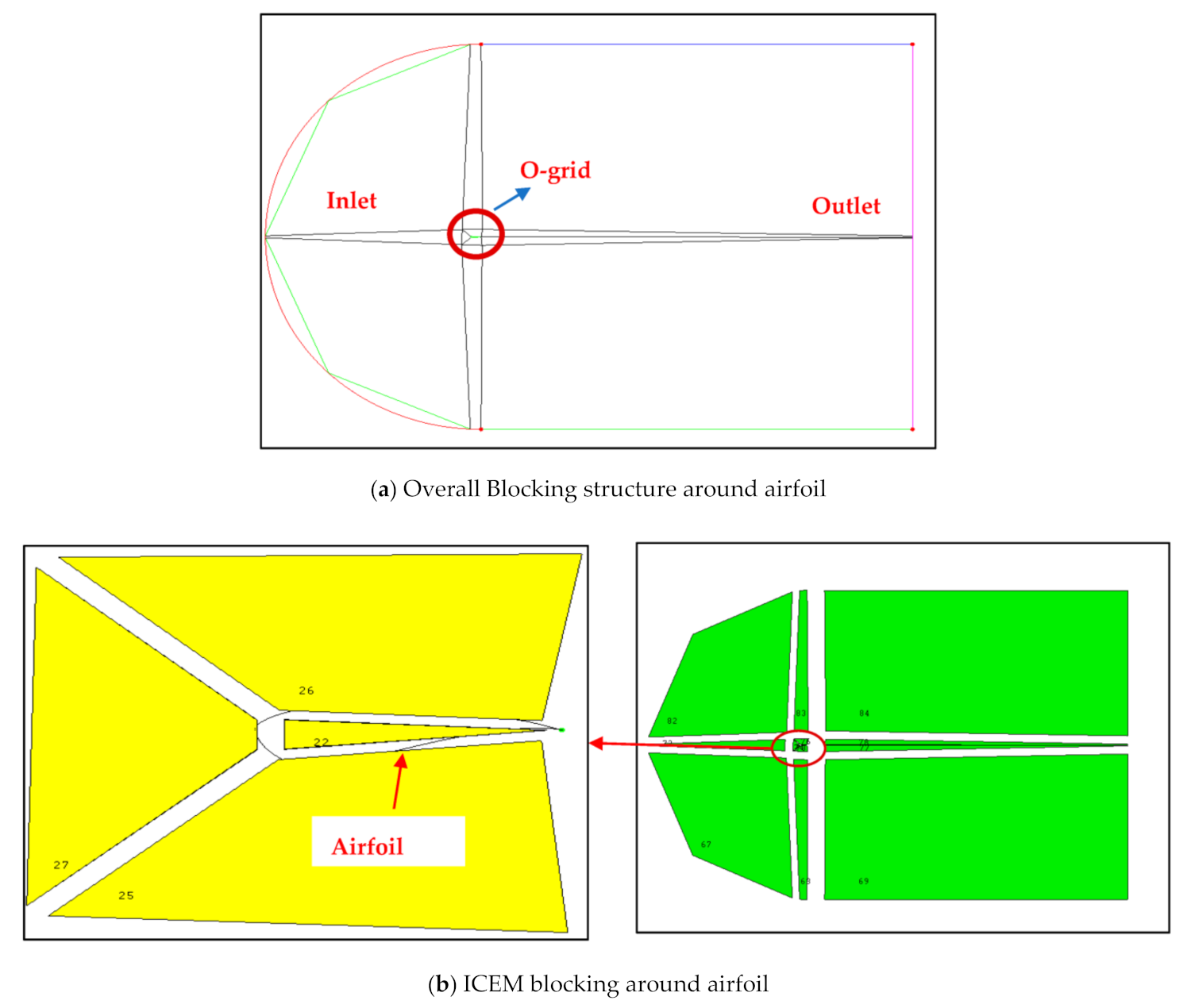
3.3. Mesh Generation

The governing equations are then discretized using ANSYS-ICEM CFD and solved inside each of the subdomains. The topology employed is based on five O-grids for the airfoil domain. The five O-grids split radially in the main block of the airfoil. The details of grid topology and the grid around the computational domain are shown in Figure 6 and Figure 7, respectively. The O-grid topology was adopted to have better and uniform control near-wall mesh and $y^{+}$ values. Values of $y^{+}$ should be less than 1 inside the domain of airfoil for the simulation to get full advantages of the SST turbulence model. However, the relation derived for the flow over a flat plate and will only provide an initial estimate of $\Delta y$ for airfoil geometry besides a flat plate. To adjust the values of $\Delta y$, very few iterations are needed to conclude the value of $\Delta y$ to get the required $y^{+}$ value for a particular set of boundary conditions.

3.4. Mesh Independence Study

The grid independence study was conducted using four grids M1, M2, M3, and M4. The details of these four grids are described in

Table 2. Mesh distribution in the CFD domain for the grid independence study.

Mesh	Nodes along Upstream	Nodes along the Leading Edge of Airfoil	Nodes along Downstream	Number of Nodes around Airfoil Length	Face Diagonal Nodes	Nodes along Trailing Edge	Nodes along the Leading Edge	Maximum Value of y+	Coefficient of Drag (Cd)	Coefficient of Lift (Cl)	Total Number of Nodes (million)	Memory Allocated by the Solver	Total CPU Time	Total Iterations at Convergence
M-i	NU	FLE	ND	NCL	FD	NT	NLE	y+	Cd	Cl	Nt	[MB]	[s]
M1	100	75	100	150	100	100	150	0.7	0.018	0.591	0.34	638	1320	300
M2	100	100	100	150	150	250	200	0.7	0.0179	0.593	0.54	989	1860	274
M3	100	125	100	150	200	300	250	0.7	0.0178	0.595	0.7	1065	2280	226
M4	100	150	100	150	250	350	300	0.7	0.0178	0.595	0.97	1203	2700	205

. Nodes along the streamwise direction $N_U, N_D$ and $N_{CL}$ were kept constant and equal for the grids. Meanwhile, nodes along the radial direction, i.e., $F_{DN}$, $N_{TE}$, and $N_{LE}$ are increased by 50 counts and $F_{LE}$ are increased by 25 counts of the initial numbers of nodes and therefore new mesh grid is generated using new grid data. Steady-state simulation of airfoil NREL S-821 was carried out for all four grids (M1–M4) at a wind speed of 34 m/s. Cd, Cl, CPU time per 10 iterations, and allocated memory by the solver for all the simulations were recorded and compared. Computational results shown in Table 2 have the same values of C_l and C_d in mesh M3 and M4. CPU time and allocated memory consumed by the mesh M3 were considerably lesser than that of mesh M4. Thus, mesh M3 was finalized based upon the consumption of CPU time for all the simulations conducted in the study. Figure 8 demonstrates the mesh topology design with its specific name in the CFD domain for grid independence study.

4. Results and Discussion

The aerodynamic shape optimization and simulation process is carried out to have an objective to decrease the horizontal aerodynamic force (minimize drag) subject to different airfoil and their structural constraints. The whole optimization process was accomplished with in-house MATLAB code. CFD and ICEM CFD were used to validate the airfoil pressure distributions and meshing, respectively, while ANSYS CFX was employed for computing the results. Blocking and framework have been created to mesh original and optimized airfoil and solve it under a given set of conditions. The design conditions, constraints, and optimization objectives are shown in

Table 3. Optimization objective and constraints.

Angle of Attack (AOA)	3°
Geometric constraints	Thickness ≈22% of chord length for NREL S-821. Thickness ≈12.5% of chord length for RAE-2822 Minimum thickness ≥1% of chord length. $T_{TE}$ and $T_{off}=0$
Aerodynamic constraint	Coefficient of drag (${\mathrm{C}}_{\mathrm{d}}$) < original airfoil S-821 & RAE-2822. Lift to drag ratio > original airfoil S-821 & RAE-2822
Objective	Minimize the coefficient of drag (${\mathrm{C}}_{\mathrm{d}}$)
Termination Condition	GA stopped based on bit string affinity value

. These optimization objectives and constraints are depicted in both the subsonic and transonic airfoil.

In total, eight design variables were used for the CST parameterization method to generate a new airfoil (S-821 and RAE-2822) shown in

Table 4. The design variables for CST.

Variables	RAE-2822	S-821
$A_l^0$	−0.1232	−0.4750
$A_l^1$	−0.1734	−0.3828
$A_l^2$	−0.1791	−0.0710
$A_l^3$	0.0586	0.1254
$A_u^0$	0.1261	0.2283
$A_u^1$	0.152	0.3335
$A_u^2$	0.2066	0.2181
$A_u^3$	0.1961	0.3586

. In the optimization process by the CST method for a 3° polynomial order, four variables for each lower and upper surface are needed to design an airfoil. The role of these design parameters is to find suitably optimized airfoil within the range of upper and lower bounds of shape coefficients. These eight design variables are important for the generation of the optimized airfoil by GA code.

4.1. Subsonic (NREL S-821) and Transonic (RAE-2822) Airfoil Design

The flow field conditions for subsonic (NREL S-821) and transonic (RAE-2822) were studied at Mach number (Ma) 0.1 and 0.7, respectively and Reynolds number (Re) was 8 million at 3° angle of attack. Total drag was minimum on the airfoil between the range of 3° to 5° angles of attack. We considered 0.34 m as chord length (c) for both the airfoil. The CST parameters play a crucial role during the optimization process in describing the shape of an airfoil. The further shape of an airfoil was defined by two curvatures of an airfoil, i.e., upper and lower parts. During the optimization process, lower and upper bound values are defined for every design variable in GA MATLAB code. As a result, the corresponding airfoil profile is generated using the best set of CST parameters produced by GA. Then the airfoil is tested at the given above condition for both subsonic and transonic airfoil. XFOIL calculates Cl, Cd, and pressure distribution on the airfoil surface which is called the in-house MATLAB program. The performance of the baseline and optimized airfoils were compared and summarized in

Table 5. Detailed XFOIL performance comparison of airfoils NREL S-821 and RAE-2822.

	NREL S-821		RAE-2822
	Original Airfoil	Optimized Airfoil	Original Airfoil	Optimized Airfoil
Cl	0.637	0.616	0.539	0.547
Cd	0.010	0.009	0.008	0.007
L/D	63.7	68.4	67.4	78.1
AOA (degree)	3°	3°	3°	3°

. As a result, it can be concluded by comparing both results obtained from XFOIL, that the optimized airfoil with eight design variables shows better results than the original subsonic NREL S-821 and transonic RAE-2822 airfoil.

From Table 5, it is observed that Cd is minimized and the L/D ratio is better for optimized airfoil on comparing with original airfoil for both NREL S-821 and RAE-2822. Since Cd for the optimized airfoil NREL S-821 is 0.009 and for RAE-2822 is 0.007 which is lower than baseline airfoil by 10% and 12%, respectively. This shows an improvement in L/D ratio by 7.4% and 15.9% for an optimized airfoil NREL S-821 and RAE-2822, respectively. The comparison of the airfoil profile between the original and the optimized airfoil NREL S-821 and RAE-2822 is demonstrated in Figure 9 and Figure 10, respectively. Figure 9 depicts that at 20% of the chord length, the optimized airfoil passes through −0.12 and the original airfoil from −0.15 at the y-axis, whereas another part of the airfoil overlaps each other. This shows that an optimized airfoil is reduced by 6% in its width of an airfoil. As a result, changes are shown in the pressure coefficient near about 20% of the chord length. The best-optimized airfoil is found whose thickest point occurs at x/c = 0.21. Figure 10 shows changes from 20% to 50% of chord length where less negative pressure is generated by a fluid in optimized airfoil compare to the original airfoil. RAE-2822 optimized airfoil is reduced by 3% of chord length and its thickest point occurs at x/c = 0.392. As a result, drag is minimized for optimized airfoil due to changes in the thickness of the airfoil.

Figure 11 demonstrates the L/D ratio concerning 3° AOA for both optimized and original airfoil. Both figures for NREL S-821 and RAE-2822 depict that the optimized airfoil has an increment in comparison to the original airfoil. By looking at the figures, it can be concluded that the lift to drag ratio is higher which implies good off-design property for small wind turbine blades.

The pressure distribution curve over the surface of the original and the optimized airfoil at 3° AOA are compared and shown in Figure 12. Lift, drag, and pressure data are calculated by XFOIL flow solver in which the C_P values are relatively high for both the optimized airfoils NREL S-821 and RAE-2822. These are the aerodynamic properties of an airfoil that are directly obtained from the given design objective. Pressure distribution across the airfoil surface calculated by XFOIL works on the panel technique method. In the panel technique method, the whole airfoil is divided into different flat panels and the near trailing and leading edges panel is increased to capture the curve perfectly. In every panel, the middle point is the control point of the panel, and the vortex is generated at the middle point of every panel. By the summations of all the vortex produced in airfoil results in the generation of lift in an upward direction perpendicular to the fluid flow. Meanwhile, drag is calculated far away from the trailing edges which are parallel to the fluid flow in opposite direction.

In Figure 12a, at 20% of the chord length, it is observed that more negative pressure is generated at the upper surface in the original airfoil than optimized airfoil due to fluid flow around the surface whereas in the lower surface of the original airfoil more pressure is generated than optimized airfoil. Due to the high-pressure generation in the original airfoil, more lift is depicted for the original airfoil compared to an optimized airfoil. However, drag is minimized in optimized airfoil due to a decrement in the thickness of the optimized airfoil. As a result, the L/D ratio shows an improvement of 7.4% in the optimized airfoil. From Figure 12b, it can be said that negative pressure is higher on the upper side of the surface of the original airfoil from 30% to 80% of the chord length whereas the lower side of the surface of the optimized airfoil has higher pressure than original airfoil RAE-2822. Therefore the lift produced by the optimized airfoil is better than the original airfoil RAE-2822. As a result, it can be concluded that the L/D ratio of an optimized airfoil is better than that of baseline airfoil RAE-2822. The optimized airfoil S-821 and RAE-2822 have a greater C_P value than the original airfoil.

The convergence graph of an optimized airfoil with six and eight design parameters is shown in Figure 13. The error bars and the pressure distribution curve at AOA 3° with regards to the number of iteration are displayed in Figure 13. The pressure residual at the surface of an airfoil is very small and the geometry residuals are below 3 × 10⁻³. The comparison of optimized results between CST (n = 6) and CST (n = 8) was done and it was concluded that the optimized airfoil with eight design CST parametric variables shows better results than six parameters variables. In the figure below, the blue and red color in the first part of every figure signifies airfoil and C_p at normalized chord length, respectively. While in the second part of each figure, yellow denotes residual error, red and blue denote the convergence plots.

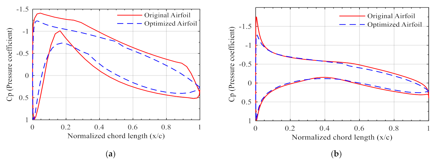
4.2. Numerical Validation

Based on CST and GA, optimized geometry and original airfoil were validated in the CFD-CFX environment using the RANS equation. One of the important motivations of this work was to make the RANS-based aerodynamic shape optimization of the airfoil with rapid changes using high-performance computing resources. Simulations were performed using the RANS model to compute the performance of the optimized airfoil along with $k-\omega$ SST turbulence model. Airfoil NREL S-821 designed by combining CST and GA optimization process was validated numerically. Simulation of airfoil NREL S-821 was done at 3° AOA and at different conditions presented in Table 1 to compare the results with the existing experimental data from reliable NREL-based data sources [38]. Some forces exerted on the airfoil are usually broken down into two different forces and moments. The total component of the net force acting perpendicular to the inflow is called lifting force, and the net force acting parallel to the inflow is called drag forces. In

Table 6. Detailed comparison of CFD performance of baseline and optimized airfoils with experimental results (NREL S-821).

	NREL S-821			Relative Variation
	Experimental Data [32]	Baseline Airfoil (CFD)	Optimized Airfoil (CFD)	Baseline with Exp.	Optimized with Baseline
Cl	0.61	0.59	0.56	−3.4%	−5.08%
Cd	0.019	0.018	0.0167	+5.50%	+7.22%
L/D	32.1	32.77	33.53	+2.1%	+2.2%
AOA	3°	3°	3°

the lift and drag coefficient of the baseline and optimized airfoil by the computational model are shown and compared with the experimental data at 3° AOA. The lift to drag ratio for an optimized airfoil is about 2.2% higher than the baseline airfoil NREL S-821 CFD data. It is observed that Cd for an optimized airfoil is 7.22% better compared with the baseline CFD results. However, on comparing baseline airfoil CFD results with the experimental data, there is a slight increment of 2.1% in the lift to drag coefficient.

Simulation outcomes of static pressure are presented in Figure 14 over the original and optimized airfoils at an angle of attack 3°. The original airfoil is shown on the left side while the optimized airfoil is displayed on the right side. Pressure over the upper surface of the original airfoil is observed more negative than that of an optimized airfoil. While there is higher pressure on the lower surface of both the original and optimized airfoil than that of the incoming flow stream. Therefore, the airfoil is effectively pushed upward, perpendicular to the incoming airflow.

The contours of velocity components at 3° AOA are shown in Figure 15. The left-hand side and right side displays initial airfoil and optimized airfoil, respectively, generated by GA code in MATLAB. After comparing the velocity on both the airfoils it was found that the upper surface experienced higher velocity compared to the lower surface of the airfoil. With the change of angle of attack the stagnation point changes for the airfoil. By increasing the angle of attack, the upper surface velocity increases and lower surface velocity decreases.

Contours of Mach number are shown in Figure 16 at 3° angle of attack over the original airfoil and optimized airfoil. The Mach number in the flow field is higher over the original airfoil than that of an optimized airfoil. This is because an optimized airfoil upper surface is much flatter than that of an original airfoil. Consequently, causes the flow to accelerate at low speed over the upper surface of the optimized airfoil. This leads to the reduction in the coefficient of drag for the optimized airfoil. This is why it allows flow at lower speed and higher pressure.

We can conclude based on the above discussion that simplified CST parametrization and GA lead to the optimized airfoil, which is the general trend of the airfoil but has better flow characteristics. As a result, it provides confidence to utilize this methodology for different shapes of airfoils. It is evident fact that the airfoil plays a basic role in designing the profile of any wind turbine blade. The shape optimization of the selected initial airfoil has an important influence on the energy harvesting operation of the wind turbine. With regards to these prospects, research also points out the possibility of applying design solutions to a series of wind turbines, namely offshore wind turbines, onshore wind turbines, and vertical axis wind turbines. Besides, the in-house code was written in MATLAB which is widely used and has many library functions that support execution. Factors such as the simplicity of the CST method and robustness of the code allow it to be easily combined with other blade design programs to optimize single or multiple airfoils along the blade span.

5. Conclusions

In this study, optimization of the aerodynamic shape for NREL S-821 and RAE-2822 airfoils was performed using CST in conjugation with GA. The optimization scheme consists of MATLAB code which further utilizes the XFOIL solver for an iterated process to achieve the resulting optimized airfoils. At the final step, CFD analysis for subsonic airfoil (NREL S-821) has been also conducted to validate the aerodynamic performance enhancement of the optimized airfoil and compared it to the NREL-based experimental data. One of the important motivations of this work was to make the RANS-based aerodynamic shape optimization of the airfoil with rapid changes using high-performance computing resources. Simulations are performed to compute the performance of the optimized airfoil geometry using RANS along with $k-\omega$ SST turbulence model. The results of the study can be summarized as:

• The drag coefficients by XFOIL for optimized NREL S-821 subsonic airfoil and RAE 2822 transonic airfoil are decreased by 10% and 12%, respectively, while the lift to drag ratios are improved by 7.4% and 15.9% at fixed 3° angle of attack.
• The proposed methodology in terms of lift to drag ratio, which is the crucial deciding factor in the wind turbine design, exhibits superior characteristics (3.5%) in aerodynamic optimization for subsonic airfoil as compared to the transonic airfoil.
• The CFD analysis of the baseline airfoil shows the improvements of 2.1% for the lift to drag ratio while comparing the airfoil with the NREL experimental results of the subsonic airfoil (NREL S-821).
• The CFD result for the lift to drag ratio for an optimized airfoil is about 2.2% higher than the baseline airfoil NREL S-821.
• The present aerodynamic shape optimization scheme is in close agreement with previous results and further applicability of the CST approach could be deployed alongside other competing optimization techniques with reasonable flexibility.

Significant reduction of a large number of design parameters offers a fewer number of genes for the candidate solution which further enables the search algorithm to act in comparatively more efficient and time-bound manners. Additionally, it can be also concluded that the aerodynamic shape optimization and the CST method can handle potential airfoils with much fewer parameters in the design space.

References

1. Chehouri, A.; Younes, R.; Ilinca, A.; Perron, J. Review of performance optimization techniques applied to wind turbines. Appl. Energy 2015, 142, 361–388. [Google Scholar] [CrossRef]
2. Saenz-Aguirre, A.; Fernandez-Gamiz, U.; Zulueta, E.; Ulazia, A.; Martinez-Rico, J. Optimal wind turbine operation by artificial neural network-based active gurney flap flow control. Sustainability 2019, 11, 2809. [Google Scholar] [CrossRef] [Green Version]
3. Rodriguez-Eguia, I.; Errasti, I.; Fernandez-Gamiz, U.; Blanco, J.M.; Zulueta, E.; Saenz-Aguirre, A. A parametric study of trailing edge flap implementation on three different airfoils through an artificial neuronal network. Symmetry 2020, 12, 828. [Google Scholar] [CrossRef]
4. Shahrokhi, A.; Jahangirian, A. Airfoil shape parameterization for optimum navier—stokes design with genetic algorithm. Aerosp. Sci. Technol. 2007, 11, 443–450. [Google Scholar] [CrossRef]
5. Zhu, W.J.; Shen, W.Z.; Sørensen, J.N. Integrated airfoil and blade design method for large wind turbines. Renew. Energy 2014, 70, 172–183. [Google Scholar] [CrossRef] [Green Version]
6. Song, W.; Keane, A.J. A Study of shape parameterisation methods for airfoil optimization. In Proceedings of the 10th AIAA/ISSMO Multidisciplinary Analysis and Optimization Conference, Albany, NY, USA, 30 August–1 September 2004; pp. 1–8. [Google Scholar]
7. Della, P.; Daniele, E.; Amato, E.D. An airfoil shape optimization technique coupling PARSEC parameterization and evolutionary algorithm. Aerosp. Sci. Technol. 2014, 32, 103–110. [Google Scholar] [CrossRef]
8. Khurana, M.; Winarto, H.; Sinha, A. Airfoil geometry parameterization through shape optimizer and computational fluid dynamics. In Proceedings of the 46th AIAA Aerospace Sciences Meeting and Exhibit, Reno, NV, USA, 7–10 January 2008; pp. 1–18. [Google Scholar]
9. Safari, M.; Ahmadabadi, M.N.; Ghaei, A.; Shirani, E. Inverse design in subsonic and transonic external flow regimes using Elastic Surface Algorithm. Comput. Fluids 2014, 102, 41–51. [Google Scholar] [CrossRef]
10. Ahmadabadi, M.N.; Ghadak, F.; Mohammadi, M. Subsonic and transonic airfoil inverse design via ball-spine algorithm. Comput. Fluids 2013, 84, 87–96. [Google Scholar] [CrossRef]
11. Saleem, A.; Kim, M.H. Effect of rotor axial position on the aerodynamic performance of an airborne wind turbine system in shell configuration. Energy Convers. Manag. 2017, 151, 587–600. [Google Scholar] [CrossRef]
12. Sripawadkul, V.; Padulo, M.; Guenov, M. A comparison of airfoil shape parameterization techniques for early design optimization. In Proceedings of the 13th AIAA/ISSMO Multidisciplinary Analysis Optimization Conference, Fort Worth, TX, USA, 13–15 September 2010; pp. 1–9. [Google Scholar]
13. Derksen, R.W.; Rogalsky, T. Advances in engineering software Bezier-PARSEC: An optimized aerofoil parameterization for design. Adv. Eng. Softw. 2010, 41, 923–930. [Google Scholar] [CrossRef]
14. Han, X.; Zingg, D.W. An adaptive geometry parametrization for aerodynamic shape optimization. Optim. Eng. 2014, 15, 69–91. [Google Scholar] [CrossRef]
15. Yang, F.; Yue, Z.; Li, L.; Yang, W. Aerodynamic optimization method based on Bezier curve and radial basis function. Proc. Inst. Mech. Eng. Part G J. Aeros Eng. 2018, 232, 459–471. [Google Scholar] [CrossRef]
16. Wu, X.; Zhang, W.; Peng, X.; Wang, Z. Benchmark aerodynamic shape optimization with the POD-based CST airfoil parametric method. Aerosp. Sci. Technol. 2019, 84, 632–640. [Google Scholar] [CrossRef]
17. Ullah, Z.; Wang, X.; Chen, Y.; Zhang, T.; Ju, H.; Zhao, Y. Time-domain output data identification model for pipeline flaw detection using blind source separation technique complexity pursuit. Acoustics 2019, 1, 13. [Google Scholar] [CrossRef] [Green Version]
18. Saleem, A.; Kim, M.H. Aerodynamic performance optimization of an airfoil-based airborne wind turbine using genetic algorithm. Energy 2020, 203. [Google Scholar] [CrossRef]
19. Samareh, J.A. Survey of shape parameterization techniques for high-fidelity multidiscplinary shape optimization. AIAA J. 2001, 39, 877–884. [Google Scholar] [CrossRef]
20. Ulaganathan, S.; Balu, R. Optimum hierarchical bezier parameterisation of arbitrary curves and surfaces. In Proceedings of the 11th Annual CFD Symposium, Bangalore, India, 11–12 August 2009; pp. 46–48. [Google Scholar]
21. Kulfan, B.M. Universal parametric geometry representation method-CST. J. Aircr. 2008, 45, 142–158. [Google Scholar] [CrossRef]
22. Kulfan, B.M.; Bussoletti, J.E. “Fundamental” parametric geometry representations for aircraft component shapes. In Proceedings of the 11th AIAA/ISSMO Multidisciplinary Analysis and Optimization Conference, Portsmouth, VA, USA, 6–8 September 2006; p. 6948. [Google Scholar]
23. Sobieczky, H. Geometry generator for CFD and applied aerodynamics. In New Design Concepts for High Speed Air Transport; Springer: Vienna, Austria, 1997; pp. 137–158. [Google Scholar]
24. Lane, K.; Marshall, D. A surface parameterization method for airfoil optimization and high lift 2D geometries utilizing the CST methodology. In Proceedings of the 47th AIAA Aerospace Sciences Meeting including The New Horizons Forum and Aerospace Exposition, Orlando, FL, USA, 5–8 January 2009. [Google Scholar] [CrossRef] [Green Version]
25. Akram, M.T.; Kim, M.-H. Aerodynamic shape optimization of NREL S809 airfoil for wind turbine blades using reynolds-averaged navier stokes model—Part II. Appl. Sci. 2021, 11, 2211. [Google Scholar] [CrossRef]
26. Lane, K.; Marshall, D. Inverse airfoil design utilizing CST parameterization. In Proceedings of the 48th AIAA Aerospace Sciences Meeting Including the New Horizons Forum and Aerospace Exposition, Orlando, Fl, USA, 4–7 January 2010. [Google Scholar] [CrossRef] [Green Version]
27. Mukesh, R.; Lingadurai, K.; Selvakumar, U. Airfoil shape optimization using non-traditional optimization technique and its validation. J. King Saud Univ. Eng. Sci. 2014, 26, 191–197. [Google Scholar] [CrossRef] [Green Version]
28. Orman, E.; Durmus, G. Comparison of shape optimization techniques coupled with genetic algorithm for a wind turbine airfoil. In Proceedings of the 2016 IEEE Aerospace Conference, Big Sky, MT, USA, 3 May–3 December 2016; pp. 1–7. [Google Scholar] [CrossRef]
29. Goldberg, D.E. Genetic Algorithms in Search, Optimization, and Machine Learning; Addison-Wesley Publishing Company: Boston, MA, USA, 1989; p. 432. [Google Scholar]
30. Chapman, S.J. MATLAB Programming for Engineers, 4th ed.; James, H., Ed.; Thomson Learning: Toronto, ON, Canada, 2008; pp. 3–251. [Google Scholar]
31. Patankar, S. Numerical Heat Transfer and Fluid Flow; Taylor: London, UK, 1980; pp. 1–197. [Google Scholar]
32. Markatos, N.C. Modelling of two-phase transient flow and combustion of granular propellants. Int. J. Multiph. Flow 1986, 12, 913–933. [Google Scholar] [CrossRef]
33. Karabelas, S.J.; Markatos, N.C. Unsteady transition from a Mach to a regular shockwave intersection. In Proceedings of the IASME/WSEAS International Conference on Fluid Dynamics and Aerodynamics, Corfu, Greece, 20–22 August 2005; pp. 168–173. [Google Scholar]
34. Karabelas, S.J.; Markatos, N.C. Water vapor condensation in forced convection flow over an airfoil. Aerosp. Sci. Technol. 2008, 12, 150–158. [Google Scholar] [CrossRef]
35. Menter, F.R. Zonal two equation k—ω turbulence models for aerodynamic flows. In Proceedings of the 24th Fluid Dynamics Conference for Aerodynamic Flows-AIAA, Orlando, FL, USA, 6–9 July 1993. [Google Scholar] [CrossRef]
36. Date, A.W. Introduction to Computational Fluid Dynamics; Cambridge University Press: Cambridge, UK, 2005. [Google Scholar]
37. Saeed, M.; Kim, M.H. Aerodynamic performance analysis of an airborne wind turbine system with NREL Phase IV rotor. Energy Convers. Manag. 2017, 134, 278–289. [Google Scholar] [CrossRef]
38. Somers, D.M. The S819, S820, and S821 airfoils. Nat. Renew. Energy Lab. 2005. [Google Scholar] [CrossRef] [Green Version]
Figure 1. Airfoil generated by CST parameterization (a) S-821 and (b) RAE-2822.
Applsci 11 03791 g001
Figure 2. Optimized airfoil shape profile.
Applsci 11 03791 g002
Figure 3. Genetic algorithm (GA) flow chart.
Applsci 11 03791 g003
Figure 4. Exchanging genes among parents to form offspring.
Applsci 11 03791 g004
Figure 5. Optimization flow chart.
Applsci 11 03791 g005
Figure 6. Blocking topology details.
Applsci 11 03791 g006
Figure 7. Meshing of the computational domain.
Applsci 11 03791 g007aApplsci 11 03791 g007b
Figure 8. Meshing design topology and its naming.
Applsci 11 03791 g008
Figure 9. Comparison of original and optimized airfoil shape (NREL S-821).
Applsci 11 03791 g009
Figure 10. The shape comparison of an original and optimized airfoil (RAE-2822).
Applsci 11 03791 g010
Figure 11. Comparison of coefficient of Lift to drag (L/D) ratio with respect to AOA (a) NREL-S821, (b) RAE-2822.
Applsci 11 03791 g011
Figure 12. Distribution of pressure over the surface of an initial and optimized airfoil (a) NREL S-821; (b) RAE-2822.
Applsci 11 03791 g012
Figure 13. The convergence process and error bars with the generation corresponding to CST method. (a) NREL S-821 (n=6), (b) NREL S-821 (n = 8), (c) RAE-2822 (n = 6), (d) RAE-2822 (n = 8).
Applsci 11 03791 g013
Figure 14. Pressure contour for the original (left) and the optimized airfoil (right) (NREL S-821).
Applsci 11 03791 g014
Figure 15. Velocity contour for original (left) and the optimized airfoil (right) (NREL S-821).
Applsci 11 03791 g015
Figure 16. Mach number contour for original (left) and the optimized airfoil (right) (NREL S-821).
Applsci 11 03791 g016