Stochastic Analysis of a Priority Standby System under Preventive Maintenance

Abstract

In this paper, we propose a system of two dissimilar units: one unit prioritizes operation (priority unit), and the other unit is kept as a cold standby (ordinary unit). In this system, we assume that the failures, repairs, and preventive maintenance (PM) times follow arbitrary distributions for both units, except for the fact that the repair time of the ordinary unit follows an exponential distribution. The priority unit has normal, partial failure or total failure modes, while the ordinary unit has normal or total failure modes. The PM of the system can be started after time t when (i) the priority unit is in the normal or partial failure modes up to time t and (ii) the standby unit is available up to time t. PM can be achieved in two types: the costlier type with probability p and the cheaper type with probability $(1-p)$. Under these assumptions, we investigate the reliability measures of the system using the regenerative point technique. Finally, we show a numerical example to illustrate the theoretical findings and show the effect of preventive maintenance in the reliability measures of the proposed system.

1. Introduction

Standby redundancy is a technique that can be used to improve and increase the reliability and availability of systems. Improvement of a standby system depends on many factors, such as the repair, preventive maintenance, and the availability of workmen.

Many authors have investigated some related problems of the reliability of a two-unit standby system assuming that the failure time for the operating unit is exponentially distributed; among those, El-Sherbeny and Al-Hussaini [1] calculated the availability and mean time to failure in the steady-state case of different configurations of series systems with exponentially distributed times. They assumed that the failure and repair times of operative and warm standby components followed exponential distribution. Kumar and Malik [2] focused on the stochastic modeling of a computer system of two identical units: one operating and the other kept as cold standby. In each, the unit hardware (h/r) and software (s/w) components work together and fail independently. They assumed the failure time distributed to be negative exponential. Sharma et al. [3] considered a cold standby system with two dissimilar units, one named priority and the other standby. They obtained some reliability measures for the system considering failure times following exponential distribution. Yusuf et al. [4] presented the reliability measures of deterioration with time.

They also studied the effect of time and deterioration rates on system reliability. Yann and Meng [5] considering a warm standby repairable system consisting of a two dissimilar units, where one unite takes priority in use if one repairman is available. They assumed that the working and repairing times followed negative exponential distribution. They illustrated the theoretical results by numerical examples and graphed the reliability measures with different parameters of failure and repair rates. El-said [6] investigated the cost–benefit analysis of a two-unit cold standby system with two stages for repair of the failed unit. Mahmoud and Moshref [7] studied the stochastic analysis of a two-unit cold standby system considering hardware failure, human error failure, and PM. Mohamoud et al. [8] discussed the system of two priority standby units under repair, post-repair, and PM. Di Nardo et al. [9] used a quantitative model based on Bhopal accident data, in which the technical, organizational, and human factors could be managed effectively with a safety management system (SMS). Wells [10] used some distributional assumptions involving distributions of phase type, introducing matrix Laplace transformations to extend the known analytic results for systems with warm standbys to the case in which the systems under study are subject to both repairable and non-repairable failures occurring in the system as a whole instead of a single operating unit. Zhong and Jin [11] discussed a novel optimal PM policy for a cold standby system with two components when a repairman is present. In their study, an SMP and regenerative point technique was used to model the system under some reasonable assumptions, and all possible states of the system and transition probabilities between them were analyzed. In addition, they derived the optimal PM cycle by maximizing the mean time from the initial state to system failure in the form of the theorem. Levitin et al. [12] considered homogeneous, cold standby systems performing missions of the fixed duration when a failure of an operating element results in a mission failure. They considered a system operating in a random environment modeled by the Poisson process of shocks. Ruiz-Castroa and Dawabshab [13] discussed a multi-state warm standby system with preventive maintenance, loss of units, and an indeterminate multiple number of repairpersons. This system can be applied to the backup server with periodic inspection by an installed monitoring program that analyzes logic and physics parameters to detect possible errors arising from internal and/or external events. Ge et al. [14] investigated the reliability analysis of a cold standby system under stepwise Poisson shocks. Gao and Wang [15] studied the reliability and availability analysis of a repairable retrial system with mixed standbys, a single repair facility subjected to preventive maintenance or active breakdown. They obtained the steady-state availability by solving the steady-state probability in matrix form. Kumar et al. [16] developed a reliability model for a non-identical cold standby system for the evaluation of system reliability, mean time to system failure, steady-state availability, the busy period of server, expected number of repairs, expected number of visits by the server, and the profit function of the system by considering all time-random variables to be Weibull distributed. Kumar and Goel [17] discussed a two-unit cold standby system by considering the concepts of degradation, inspection, preventive maintenance (PM), and priority. They considered the unit to work at a reduced capacity after its repair and thus called it a degraded unit. Furthermore, they discussed various reliability characteristics, such as mean time to system failure (MTSF), availability, busy period of the repairman, expected number of visits by the repairman, and profits of the system. Hirata et al. [18] addressed a derivation procedure for the reliability function of the two-component priority standby redundant system based on the maximum entropy principle. The procedure based on the maximum entropy principle in information theory is widely known as an elegant approach to deriving a probability density function by utilizing the given information about the stochastic property of random variables. Kumar [19] analyzed the cost–benefit analysis of a cold standby repairable system under varying environmental conditions: normal and abnormal. Kumar and Chowdhary [20] investigated the stochastic analysis of an identical two-unit standby system model with the concept of preventive maintenance of the operative unit after some significant time, which is considered to be a random variable with some probability distribution.

In this paper, we propose a system of two dissimilar units: one prioritizes operation, while the other can be kept as a standby unit. In addition, we assume that there are two types of PM for the priority unit, namely, the costlier type with probability p and the cheaper type with probability $(1-p)$. All of the failures, repairs, and PM times are arbitrary distributed, except for the repair time of the ordinary unit, which is exponentially distributed. In addition, we assume that the priority unit has normal, partial failure or total failure modes. Next, we use the regenerative point technique to investigate the performance of the proposed system in the steady-state case in terms of some reliability measures: (i) the mean time to system failure (MTSF); (ii) availability; (iii) busy periods with repair due to repair and PM; (iv) the profit gain of the system. Finally, in order to show the effect of PM and system parameters on the reliability measures of the proposed system, we provide some numerical illustrations and graphs.

2. System Description

• The system consists of two dissimilar units: one is a priority unit and the other is the ordinary unit.
• The priority unit has three modes, namely, normal, total, and partial failures, while the ordinary unit has two modes, normal and total failure.
• Initially, the priority unit is in normal mode operation, while the ordinary unit can be kept as a standby case (cold standby).
• If the priority unit is in normal mode until time t without total (or partial) failures, then it should go to the PM (costlier with probability p and cheaper with probability $(1-p)$) provided that the standby unit is available. On the other hand, if the priority unit is in the partial failure mode until time t (without total failure), it should go to costlier PM provided that the standby unit is available. In all cases, when the standby unit is not available, then PM is postponed until the next time period of PM.
• The switchover is perfect and instantaneous and only one the server operator is available for both of the repairs and PM.
• All of the time distributions are arbitrary except the repair time of the ordinary unit.
• After repair or PM, the unit returns back to normal mode.

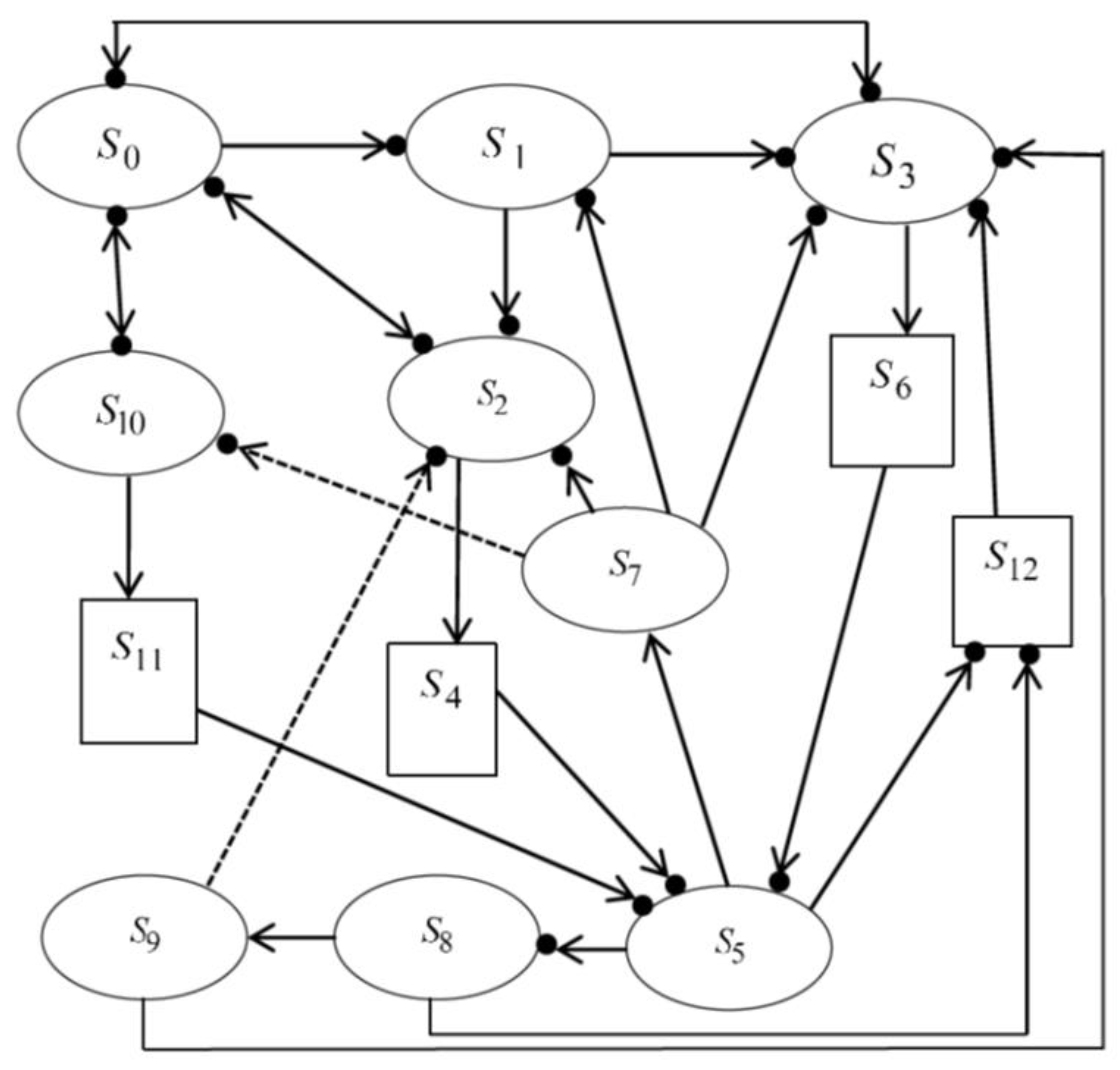
System States

The configuration and states of the proposed system can be descried through the following notations:

$N_O/N_{OC}/N_{pf}$:	the unit is in normal mode/in normal mode and is continued from the
$/N_{Pf}/N_s$	earlier state/in partial failure mode/in partial failure mode and
	is continued from the earlier state/in normal mode and is kept
	as cold standby.
$F_r/F_R/F_{wr}$:	the unit is in failure mode and under repair/the unit in failure mode and
	under repair is continued from the earlier state state/in failure mode
	and waiting for repair.
$N_{co}/N_{ch}$:	the unit is in normal mode and under costlier PM/in normal mode and
	under cheaper PM.
$N_{Co}/N_{Ch}$:	the unit in normal mode and under costlier PM is continued from
	the earlier state/the unit in normal mode and under cheaper
	PM is continued from the earlier state.

By using these notations, the system can be presented in any one of the following states, where the first argument represents the state of the priority unit and the second argument represents the state of the ordinary unit:

$S_0=(N_o,N_s)$		$S_1=(N_{pf},N_s)$		$S_2=(N_{co},N_o)$		$S_3=(F_r,N_o)$
$S_4=(N_{Co},F_{wr})$		$S_5=(N_o,F_r)$		$S_6=(F_R,F_{wr})$		$S_7=(N_{oc},N_s)$
$S_8=(N_{pf},F_R)$		$S_9=(N_{Pf},N_s)$		$S_{10}=(N_{ch},N_o)$		$S_{11}=(N_{Ch},F_{wr})$
$S_{12}=(F_{wr},F_R).$

The up states in this system are $S_0,S_1,S_2,S_3,S_5,S_7,S_8,S_9$, and $S_{10}$; the down states are $S_4,S_6,S_{11}$, and $S_{12}$. Additionally, the states $S_0,S_1,S_2,S_3,S_5,S_8,S_{10}$ and $S_{12}$ are regenerative states, but $S_4,S_6,S_7,S_9$, and $S_{11}$ are non-regenerative states; see Figure 1.

In this this section, we calculate the transition probabilities between the different states of the system and the corresponding sojourn times for such states. From the system setup, it can be observed that the epochs of entry into any of the states $S_i\in E$ are regenerative points. $T_0(\equiv 0),T_1,T_2,\dots$ denotes the epochs at which the system enters any state $S_i\in E$, and $X_n$ denotes the state visited at epoch $T_n+$, i.e., just after transition at $T_n$. $\{X_n,T_n\}$ is the Markov renewal process with state space E, and

$$\begin{array}{c}\hfill Q_{ij}\left(t\right)=P(X_{n+1}=j,T_{n+1}-T_n\le t\mid X_n=i),\end{array}$$

is the semi-Markov kernel over E.

Thus, the transition probability matrix of embedded Markov chain is

$$\begin{array}{c}\hfill P=\left(p_{ij}\right)=(Q_{ij}(\infty )=Q(\infty )),\end{array}$$

with non-zero elements $p_{ij}$, which can be calculated by using the following probabilistic arguments:

$$\begin{array}{c}\hfill p_{01}=\int \overline{A}\left(t\right){\overline{F}}_2\left(t\right)d{F}_1\left(t\right),\end{array}$$

where $p_{01}$ means that the total failure of the priority unit does not occur until time t; PM does is achieved until time t; and partial failure of the priority unit occurs at time t. All other transition probabilities listed below can be explained in the same manner.

$$\begin{array}{ccc}\hfill p_{02}& =& p\int {\overline{F}}_1\left(t\right){\overline{F}}_2\left(t\right)dA\left(t\right),p_{03}=\int \overline{A}\left(t\right){\overline{F}}_1\left(t\right)d{F}_2\left(t\right),\hfill \\ \hfill p_{010}& =& (1-p)\int {\overline{F}}_1\left(t\right){\overline{F}}_2\left(t\right)dA\left(t\right),\hfill \\ \hfill p_{12}& =& \int {\overline{F}}_3\left(t\right)dA\left(t\right),p_{13}=\int \overline{A}\left(t\right)d{F}_3\left(t\right),\hfill \\ \hfill p_{20}& =& \int {\overline{F}}_4\left(t\right)d{B}_1\left(t\right),p_{25}^{\left(4\right)}=\int F_4\left(t\right)d{B}_1\left(t\right),\hfill \\ \hfill p_{30}& =& \int {\overline{F}}_4\left(t\right)dG\left(t\right),p_{35}^{\left(6\right)}=\int F_4\left(t\right)dG\left(t\right),\hfill \\ \hfill p_{51}^{\left(7\right)}& =& \int \overline{A}\left(t\right)(1-e^{-\delta t}){\overline{F}}_2\left(t\right)d{F}_1\left(t\right)+\delta \int {\overline{F}}_2\left(t\right)\left({\int }_0^{t}A\left(x\right)e^{-\delta x}dx\right)d{F}_1\left(t\right),\hfill \\ \hfill p_{53}^{\left(7\right)}& =& \int \overline{A}\left(t\right)(1-e^{-\delta t}){\overline{F}}_1\left(t\right)d{F}_2\left(t\right)+\delta \int {\overline{F}}_1\left(t\right)\left({\int }_0^{t}A\left(x\right)e^{-\delta x}dx\right)d{F}_2\left(t\right),\hfill \\ \hfill p_{52}^{\left(7\right)}& =& p\int (1-e^{-\delta t}){\overline{F}}_1\left(t\right){\overline{F}}_2\left(t\right)dA\left(t\right),p_{5,10}^{\left(7\right)}=(1-p)\int (1-e^{-\delta t}){\overline{F}}_1\left(t\right){\overline{F}}_2\left(t\right)dA\left(t\right),\hfill \\ \hfill p_{58}& =& \int e^{-\delta t}{\overline{F}}_2\left(t\right)d{F}_1\left(t\right),p_{5,12}=\int e^{-\delta t}{\overline{F}}_1\left(t\right)d{F}_2\left(t\right),\hfill \\ \hfill p_{83}^{\left(9\right)}& =& \int \overline{A}\left(t\right)(1-e^{-\delta t})d{F}_3\left(t\right)+\delta \int \left({\int }_0^{t}A\left(x\right)e^{-\delta t}dx\right)d{F}_3\left(t\right),\hfill \\ \hfill p_{82}^{\left(9\right)}& =& \int {\overline{F}}_3\left(t\right)(1-e^{-\delta t})dA\left(t\right),p_{8,12}=\int e^{-\delta t}d{F}_3\left(t\right),\hfill \\ \hfill p_{10,0}& =& \int {\overline{F}}_4\left(t\right)d{B}_2\left(t\right),p_{10,5}^{\left(11\right)}=\int F_4\left(t\right)d{B}_2\left(t\right).\hfill \end{array}$$

The above transition probabilities satisfy the following relations:

$$\begin{array}{ccc}& & p_{01}+p_{02}+p_{03}+p_{0,10}=1,p_{12}+p_{13}=1,p_{20}+p_{25}^{\left(4\right)}=1,\hfill \\ & & p_{30}+p_{35}^{\left(6\right)}=1,p_{51}^{\left(7\right)}+p_{52}^{\left(7\right)}+p_{53}^{\left(7\right)}+p_{5,10}^{\left(7\right)}+p_{58}+p_{5,12}=1,\hfill \\ & & p_{82}^{\left(9\right)}+p_{83}^{\left(9\right)}+p_{8,12}=1,p_{10,0}+p_{10,5}^{\left(11\right)}=1,p_{12,3}=1.\hfill \end{array}$$

In addition, the mean sojourn times of the system ${\mu }_i$ in state $S_i\in E$ can be calculated as follows:

$$\begin{array}{ccc}& & {\mu }_0=\int {\overline{F}}_1\left(t\right){\overline{F}}_2\left(t\right)\overline{A}\left(t\right)dt,{\mu }_1=\int \overline{A}\left(t\right){\overline{F}}_3\left(t\right)dt,\hfill \\ & & {\mu }_2=\int {\overline{B}}_1\left(t\right){\overline{F}}_4\left(t\right)dt,{\mu }_3=\int {\overline{F}}_4\left(t\right)\overline{G}\left(t\right)dt,\hfill \\ & & {\mu }_5=\int {\overline{F}}_1\left(t\right){\overline{F}}_2\left(t\right)e^{-\delta t}dt,{\mu }_8=\int e^{-\delta t}{\overline{F}}_3\left(t\right)dt,\hfill \\ & & {\mu }_{10}=\int {\overline{B}}_2\left(t\right){\overline{F}}_4\left(t\right)dt,{\mu }_{12}=\frac{1}{\delta }.\hfill \end{array}$$

3. Mean Time to System Failure

In this section, we derive the mean time to system failure as one of the reliability measures of the proposed system. According to the arguments of theory of regenerative processes, the mean times to system failure ${\overline{\mathsf{\Pi }}}_i\left(t\right)$ starting from state $S_i\in E,i=0,1,2,3,10$ can be obtained by solving the following equations:

$$\begin{array}{ccc}\hfill {\overline{\mathsf{\Pi }}}_0\left(t\right)& =& {\overline{F}}_1\left(t\right){\overline{F}}_2\left(t\right)\overline{A}\left(t\right)+q_{01}\left(t\right)\mathsf{\copyright }{\overline{\mathsf{\Pi }}}_1\left(t\right)+q_{02}\left(t\right)\mathsf{\copyright }{\overline{\mathsf{\Pi }}}_2\left(t\right)\hfill \\ & +& q_{03}\left(t\right)\mathsf{\copyright }{\overline{\mathsf{\Pi }}}_3\left(t\right)+q_{0,10}\left(t\right)\mathsf{\copyright }{\overline{\mathsf{\Pi }}}_{10}\left(t\right),\hfill \end{array}$$

(1)

$$\begin{array}{ccc}\hfill {\overline{\mathsf{\Pi }}}_1\left(t\right)& =& {\overline{F}}_3\left(t\right)\overline{A}\left(t\right)+q_{12}\left(t\right)\mathsf{\copyright }{\overline{\mathsf{\Pi }}}_1\left(t\right)+q_{13}\left(t\right)\mathsf{\copyright }{\overline{\mathsf{\Pi }}}_3\left(t\right),\hfill \end{array}$$

(2)

$$\begin{array}{ccc}\hfill {\overline{\mathsf{\Pi }}}_2\left(t\right)& =& {\overline{B}}_1\left(t\right){\overline{F}}_4\left(t\right)+q_{20}\left(t\right)\mathsf{\copyright }{\overline{\mathsf{\Pi }}}_0\left(t\right),\hfill \end{array}$$

(3)

$$\begin{array}{ccc}\hfill {\overline{\mathsf{\Pi }}}_3\left(t\right)& =& {\overline{F}}_4\left(t\right)\overline{G}\left(t\right)+q_{30}\left(t\right)\mathsf{\copyright }{\overline{\mathsf{\Pi }}}_0\left(t\right),\hfill \end{array}$$

(4)

$$\begin{array}{ccc}\hfill {\overline{\mathsf{\Pi }}}_{10}\left(t\right)& =& {\overline{B}}_2\left(t\right){\overline{F}}_4\left(t\right)+q_{10,0}\left(t\right)\mathsf{\copyright }{\overline{\mathsf{\Pi }}}_0\left(t\right).\hfill \end{array}$$

(5)

By making use of Laplace transform (LT) for Equations (1)–(5) and solving for ${\overline{\mathsf{\Pi }}}_0^{*}\left(s\right)$, considering $s=0$, we obtain the time to system failure $MTSF$ in the steady state starting from the state $S_0$ as follows:

$$\begin{array}{c}\hfill MTSF=E\left(T\right)=\frac{{\mathit{N}}_{\mathit{0}}}{D_0},\end{array}$$

(6)

where

$$\begin{array}{ccc}\hfill {\mathit{N}}_{\mathit{0}}& =& {\mu }_0+p_{01}{\mu }_1+(p_{01}{p}_{12}+p_{02}){\mu }_2+(p_{01}{p}_{13}+p_{03}){\mu }_3+p_{0,10}{\mu }_{10},\hfill \end{array}$$

(7)

$$\begin{array}{ccc}\hfill D_0& =& 1-\left[p_{01}(p_{12}{p}_{20}+p_{13}{p}_{30})+p_{02}{p}_{20}+p_{03}{p}_{30}+p_{0,10}{p}_{10,0}\right].\hfill \end{array}$$

(8)

4. Availability Analysis

In this section, we discuss the pointwise and steady-state availability of the proposed system. Upon use of some probabilistic arguments, we obtain the following recursive relations for $A{V}_i\left(t\right)$, $i=0,1,2,3,5,8,10,12$, where

$$\begin{array}{ccc}\hfill A{V}_0\left(t\right)& =& M_0\left(t\right)+q_{01}\left(t\right)\mathsf{\copyright }A{V}_1\left(t\right)+q_{02}\left(t\right)\mathsf{\copyright }A{V}_2\left(t\right)+q_{03}\left(t\right)\mathsf{\copyright }A{V}_3\left(t\right)\hfill \\ & +& q_{0,10}\left(t\right)\mathsf{\copyright }A{V}_{10}\left(t\right),\hfill \end{array}$$

(9)

$$\begin{array}{ccc}\hfill A{V}_1\left(t\right)& =& M_1\left(t\right)+q_{12}\left(t\right)\mathsf{\copyright }A{V}_2\left(t\right)+q_{13}\left(t\right)\mathsf{\copyright }A{V}_3\left(t\right),\hfill \end{array}$$

(10)

$$\begin{array}{ccc}\hfill A{V}_2\left(t\right)& =& M_2\left(t\right)+q_{20}\left(t\right)\mathsf{\copyright }A{V}_0\left(t\right)+q_{25}^{\left(4\right)}\left(t\right)\mathsf{\copyright }A{V}_5\left(t\right),\hfill \end{array}$$

(11)

$$\begin{array}{ccc}\hfill A{V}_3\left(t\right)& =& M_3\left(t\right)+q_{30}\left(t\right)\mathsf{\copyright }A{V}_0\left(t\right)+q_{35}^{\left(6\right)}\left(t\right)\mathsf{\copyright }A{V}_5\left(t\right),\hfill \end{array}$$

(12)

$$\begin{array}{ccc}\hfill A{V}_5\left(t\right)& =& M_5\left(t\right)+q_{51}^{\left(7\right)}\left(t\right)\mathsf{\copyright }A{V}_1\left(t\right)+q_{52}^{\left(7\right)}\left(t\right)\mathsf{\copyright }A{V}_2\left(t\right)+q_{53}^{\left(7\right)}\left(t\right)\mathsf{\copyright }A{V}_3\left(t\right)\hfill \\ & +& q_{5,8}\left(t\right)\mathsf{\copyright }A{V}_8\left(t\right)+q_{5,10}^{\left(7\right)}\left(t\right)\mathsf{\copyright }A{V}_{10}\left(t\right)+q_{5,12}\left(t\right)\mathsf{\copyright }A{V}_{12}\left(t\right),\hfill \end{array}$$

(13)

$$\begin{array}{ccc}\hfill A{V}_8\left(t\right)& =& M_8\left(t\right)+q_{82}^{\left(9\right)}\left(t\right)\mathsf{\copyright }A{V}_2\left(t\right)+q_{83}^{\left(9\right)}\left(t\right)\mathsf{\copyright }A{V}_3\left(t\right)+q_{8,12}\left(t\right)\mathsf{\copyright }A{V}_{12}\left(t\right),\hfill \end{array}$$

(14)

$$\begin{array}{ccc}\hfill A{V}_{10}\left(t\right)& =& M_{10}\left(t\right)+q_{10,0}\left(t\right)\mathsf{\copyright }A{V}_0\left(t\right)+q_{10,5}^{\left(11\right)}\left(t\right)\mathsf{\copyright }A{V}_5\left(t\right),\hfill \end{array}$$

(15)

$$\begin{array}{ccc}\hfill A{V}_{12}\left(t\right)& =& q_{12,3}\left(t\right)\mathsf{\copyright }A{V}_3\left(t\right),\hfill \end{array}$$

(16)

where

$$\begin{array}{ccc}\hfill M_0\left(t\right)& =& {\overline{F}}_1\left(t\right){\overline{F}}_2\left(t\right)\overline{A}\left(t\right),M_1\left(t\right)={\overline{F}}_3\left(t\right)\overline{A}\left(t\right),\hfill \\ \hfill M_2\left(t\right)& =& {\overline{F}}_4\left(t\right){\overline{B}}_1\left(t\right),M_3\left(t\right)={\overline{F}}_4\left(t\right)\overline{G}\left(t\right),\hfill \\ \hfill M_5\left(t\right)& =& {\overline{F}}_1\left(t\right){\overline{F}}_2\left(t\right){\overline{G}}_1\left(t\right)+{\overline{F}}_1\left(t\right){\overline{F}}_2\left(t\right){\int }_0^t\overline{A}\left(x\right)d{G}_1\left(x\right)+{\overline{F}}_1\left(t\right){\overline{F}}_2\left(t\right)G_1\left(t\right)\overline{A}\left(t\right),\hfill \\ \hfill M_8\left(t\right)& =& {\overline{F}}_3\left(t\right){\overline{G}}_1\left(t\right)+{\overline{F}}_3\left(t\right){\int }_0^t\overline{A}\left(x\right)d{G}_1\left(x\right)+{\overline{F}}_3\left(t\right)G_1\left(t\right)\overline{A}\left(t\right),M_{10}\left(t\right)={\overline{F}}_4\left(t\right){\overline{B}}_2\left(t\right).\hfill \end{array}$$

Applying LT to (9)–(16) and solving for $A{V}_0^{*}\left(s\right)$, we obtain the steady-state availability of the system $A{V}_0(\infty )$ as follows:

$$\begin{array}{c}\hfill A{V}_0(\infty )=\underset{s\to 0}{lim}sA{V}_0^{*}\left(s\right)=\frac{\mathit{N}}{D},\end{array}$$

(17)

where

$$\begin{array}{c}\hfill N=\left|\begin{array}{cccccccc}{\mu }_0& p_{01}& p_{02}& p_{03}& 0& 0& p_{0,10}& 0\\ {\mu }_1& 1& p_{12}& p_{13}& 0& 0& 0& 0\\ {\mu }_2& 0& 1& 0& p_{25}^{\left(4\right)}& 0& 0& 0\\ {\mu }_3& 0& 0& 1& p_{35}^{\left(6\right)}& 0& 0& 0\\ {\mu }_5& p_{51}^{\left(7\right)}& p_{52}^{\left(7\right)}& p_{53}^{\left(7\right)}& 1& p_{58}& p_{5,10}^{\left(7\right)}& p_{5,12}\\ {\mu }_8& 0& p_{82}^{\left(9\right)}& p_{83}^{\left(9\right)}& 0& 1& 0& p_{8,12}\\ {\mu }_{10}& 0& 0& 0& p_{10,5}^{\left(11\right)}& 0& 1& 0\\ 0& 0& 0& p_{12,3}& 0& 0& 0& 1\\ \end{array}\right|,\end{array}$$

(18)

and D can be obtained using the differentiation of the determinant as follows:

$$\begin{array}{c}\hfill D=\sum _{j=1}^8{D}_j,\end{array}$$

(19)

where

$$D_1=\left|\begin{array}{cccccccc}0& {\mu }_{01}& {\mu }_{02}& {\mu }_{03}& 0& 0& {\mu }_{0,10}& 0\\ 0& 1& p_{12}& p_{13}& 0& 0& 0& 0\\ p_{20}& 0& 1& 0& p_{25}^{\left(4\right)}& 0& 0& 0\\ p_{30}& 0& 0& 1& p_{35}^{\left(6\right)}& 0& 0& 0\\ 0& p_{51}^{\left(7\right)}& p_{52}^{\left(7\right)}& p_{53}^{\left(7\right)}& 1& p_{58}& p_{5,10}& p_{5,12}\\ 0& 0& p_{82}^{\left(9\right)}& p_{83}^{\left(9\right)}& 0& 1& 0& p_{8,12}\\ p_{10,0}& 0& 0& 0& p_{10,5}^{\left(11\right)}& 0& 1& 0\\ 0& 0& 0& p_{12,3}& 0& 0& 0& 1\\ \end{array}\right|,$$

$$D_2=\left|\begin{array}{cccccccc}1& p_{01}& p_{02}& p_{03}& 0& 0& p_{0,10}& 0\\ 0& 0& {\mu }_{12}& {\mu }_{13}& 0& 0& 0& 0\\ p_{20}& 0& 1& 0& p_{25}^{\left(4\right)}& 0& 0& 0\\ p_{30}& 0& 0& 1& p_{35}^{\left(6\right)}& 0& 0& 0\\ 0& p_{51}^{\left(7\right)}& p_{52}^{\left(7\right)}& p_{53}^{\left(7\right)}& 1& p_{58}& p_{5,10}& p_{5,12}\\ 0& 0& p_{82}^{\left(9\right)}& p_{83}^{\left(9\right)}& 0& 1& 0& p_{8,12}\\ p_{10,0}& 0& 0& 0& p_{10,5}^{\left(11\right)}& 0& 1& 0\\ 0& 0& 0& p_{1,23}& 0& 0& 0& 1\\ \end{array}\right|,$$

$$D_3=\left|\begin{array}{cccccccc}1& p_{01}& p_{02}& p_{03}& 0& 0& p_{0,10}& 0\\ 0& 1& p_{12}& p_{13}& 0& 0& 0& 0\\ {\mu }_{20}& 0& 0& 0& {\mu }_{25}^{\left(4\right)}& 0& 0& 0\\ p_{30}& 0& 0& 1& p_{35}^{\left(6\right)}& 0& 0& 0\\ 0& p_{51}^{\left(7\right)}& p_{52}^{\left(7\right)}& p_{53}^{\left(7\right)}& 1& p_{58}& p_{5,10}& p_{5,12}\\ 0& 0& p_{82}^{\left(9\right)}& p_{83}^{\left(9\right)}& 0& 1& 0& p_{8,12}\\ p_{10,0}& 0& 0& 0& p_{10,5}^{\left(11\right)}& 0& 1& 0\\ 0& 0& 0& p_{1,23}& 0& 0& 0& 1\\ \end{array}\right|,$$

$$D_4=\left|\begin{array}{cccccccc}1& p_{01}& p_{02}& p_{03}& 0& 0& p_{0,10}& 0\\ 0& 1& p_{12}& p_{13}& 0& 0& 0& 0\\ p_{21}& 0& 1& 0& p_{25}^{\left(4\right)}& 0& 0& 0\\ {\mu }_{30}& 0& 0& 0& {\mu }_{36}^{\left(5\right)}& 0& 0& 0\\ 0& p_{51}^{\left(7\right)}& p_{52}^{\left(7\right)}& p_{53}^{\left(7\right)}& 1& p_{58}& p_{5,10}& p_{5,12}\\ 0& 0& p_{82}^{\left(9\right)}& p_{83}^{\left(9\right)}& 0& 1& 0& p_{8,12}\\ p_{10,0}& 0& 0& 0& p_{10,5}^{\left(11\right)}& 0& 1& 0\\ 0& 0& 0& p_{12,3}& 0& 0& 0& 1\\ \end{array}\right|,$$

$$D_5=\left|\begin{array}{cccccccc}1& p_{01}& p_{02}& p_{03}& 0& 0& p_{0,10}& 0\\ 0& 1& p_{12}& p_{13}& 0& 0& 0& 0\\ p_{20}& 0& 1& 0& p_{25}^{\left(4\right)}& 0& 0& 0\\ p_{30}& 0& 0& 1& p_{35}^{\left(6\right)}& 0& 0& 0\\ 0& {\mu }_{51}^{\left(7\right)}& {\mu }_{52}^{\left(7\right)}& {\mu }_{53}^{\left(7\right)}& 0& {\mu }_{58}& {\mu }_{510}& {\mu }_{512}\\ 0& 0& p_{82}^{\left(9\right)}& p_{83}^{\left(9\right)}& 0& 1& 0& p_{8,12}\\ p_{10,0}& 0& 0& 0& p_{10,5}^{\left(11\right)}& 0& 1& 0\\ 0& 0& 0& p_{12,3}& 0& 0& 0& 1\\ \end{array}\right|,$$

$$D_6=\left|\begin{array}{cccccccc}1& p_{01}& p_{02}& p_{03}& 0& 0& p_{0,10}& 0\\ 0& 1& p_{12}& p_{13}& 0& 0& 0& 0\\ p_{20}& 0& 1& 0& p_{25}^{\left(4\right)}& 0& 0& 0\\ p_{30}& 0& 0& 1& p_{35}^{\left(6\right)}& 0& 0& 0\\ 0& p_{51}^{\left(7\right)}& p_{52}^{\left(7\right)}& p_{53}^{\left(7\right)}& 1& p_{58}& p_{5,10}& p_{5,12}\\ 0& 0& {\mu }_{82}^{\left(9\right)}& {\mu }_{83}^{\left(9\right)}& 0& 0& 0& {\mu }_{8,12}\\ p_{10,0}& 0& 0& 0& p_{10,5}^{\left(11\right)}& 0& 1& 0\\ 0& 0& 0& p_{12,3}& 0& 0& 0& 1\\ \end{array}\right|,$$

$$D_7=\left|\begin{array}{cccccccc}1& p_{01}& p_{02}& p_{03}& 0& 0& p_{0,10}& 0\\ 0& 1& p_{12}& p_{13}& 0& 0& 0& 0\\ p_{20}& 0& 1& 0& p_{25}^{\left(4\right)}& 0& 0& 0\\ p_{30}& 0& 0& 1& p_{35}^{\left(6\right)}& 0& 0& 0\\ 0& p_{51}^{\left(7\right)}& p_{52}^{\left(7\right)}& p_{53}^{\left(7\right)}& 1& p_{58}& p_{5,10}& p_{5,12}\\ 0& 0& p_{82}^{\left(9\right)}& p_{83}^{\left(9\right)}& 0& 1& 0& p_{8,12}\\ {\mu }_{10,0}& 0& 0& 0& {\mu }_{10,5}^{\left(11\right)}& 0& 0& 0\\ 0& 0& 0& p_{12,3}& 0& 0& 0& 1\\ \end{array}\right|,$$

$$D_8=\left|\begin{array}{cccccccc}1& p_{01}& p_{02}& p_{03}& 0& 0& p_{0,10}& 0\\ 0& 1& p_{12}& p_{13}& 0& 0& 0& 0\\ p_{20}& 0& 1& 0& p_{25}^{\left(4\right)}& 0& 0& 0\\ p_{30}& 0& 0& 1& p_{35}^{\left(6\right)}& 0& 0& 0\\ 0& p_{51}^{\left(7\right)}& p_{52}^{\left(7\right)}& p_{53}^{\left(7\right)}& 1& p_{58}& p_{5,10}& p_{5,12}\\ 0& 0& p_{82}^{\left(9\right)}& p_{83}^{\left(9\right)}& 0& 1& 0& p_{8,12}\\ p_{10,0}& 0& 0& 0& p_{10,5}^{\left(11\right)}& 0& 1& 0\\ 0& 0& 0& {\mu }_{12}& 0& 0& 0& 0\\ \end{array}\right|,$$

$$\begin{array}{ccc}\hfill {\mu }_{01}& =& {\int }_0^{\infty }t\overline{A}\left(t\right)\overline{F_2}\left(t\right)d{F}_1\left(t\right),{\mu }_{03}={\int }_0^{\infty }t\overline{A}\left(t\right)\overline{F_1}\left(t\right)d{F}_2\left(t\right),\hfill \\ \hfill {\mu }_{02}& =& p{\int }_0^{\infty }t{\overline{F}}_1\left(t\right)\overline{F_2}\left(t\right)dA\left(t\right),{\mu }_{010}=(1-p){\int }_0^{\infty }t{\overline{F}}_1\left(t\right)\overline{F_2}\left(t\right)dA\left(t\right),\hfill \\ \hfill {\mu }_{12}& =& {\int }_0^{\infty }t{\overline{F}}_3\left(t\right)dA\left(t\right),{\mu }_{13}={\int }_0^{\infty }t\overline{A}\left(t\right)d{F}_3\left(t\right),\hfill \\ \hfill {\mu }_{20}& =& {\int }_0^{\infty }t{\overline{F}}_4\left(t\right)d{B}_1\left(t\right),{\mu }_{25}^{\left(4\right)}={\int }_0^{\infty }t{F}_4\left(t\right)d{B}_1\left(t\right),\hfill \\ \hfill {\mu }_{30}& =& {\int }_0^{\infty }t{\overline{F}}_4\left(t\right)dG\left(t\right),{\mu }_{35}^{\left(6\right)}={\int }_0^{\infty }t{F}_4\left(t\right)dG\left(t\right),\hfill \\ \hfill {\mu }_{10,0}& =& {\int }_0^{\infty }t{\overline{F}}_4\left(t\right)d{B}_2\left(t\right),{\mu }_{10,5}^{\left(11\right)}={\int }_0^{\infty }t{F}_4\left(t\right)d{B}_2\left(t\right),\hfill \\ \hfill {\mu }_{53}^{\left(7\right)}& =& {\int }_0^{\infty }t\overline{A}\left(t\right)(1-e^{-\delta })\overline{F_1}\left(t\right)d{F}_2\left(t\right)+\delta {\int }_0^{\infty }t\overline{F_1}\left(t\right)\left({\int }_0^{t}A\left(x\right)e^{-\delta x}dx\right)d{F}_2\left(t\right),\hfill \\ \hfill {\mu }_{51}^{\left(7\right)}& =& {\int }_0^{\infty }t\overline{A}\left(t\right)(1-e^{-\delta t})\overline{F_2}\left(t\right)d{F}_1\left(t\right)+\delta {\int }_0^{\infty }t\overline{F_2}\left(t\right)\left({\int }_0^{t}A\left(x\right)e^{-\delta x}dx\right)d{F}_1\left(t\right),\hfill \\ \hfill {\mu }_{52}^{\left(7\right)}& =& p{\int }_0^{\infty }t(1-e^{-\delta t})\overline{F_1}\left(t\right)\overline{F_2}\left(t\right)dA\left(t\right),\hfill \\ \hfill {\mu }_{510}^{\left(7\right)}& =& (1-p){\int }_0^{\infty }t(1-e^{-\delta t})\overline{F_1}\left(t\right)\overline{F_2}\left(t\right)dA\left(t\right),\hfill \\ \hfill {\mu }_{58}& =& {\int }_0^{\infty }t{e}^{-\delta t}\overline{F_2}\left(t\right)d{F}_1\left(t\right),{\mu }_{512}={\int }_0^{\infty }t{e}^{-\delta t}\overline{F_1}\left(t\right)d{F}_2\left(t\right),\hfill \\ \hfill {\mu }_{83}^{\left(9\right)}& =& {\int }_0^{\infty }t\overline{A}\left(t\right)(1-e^{-\delta t})d{F}_3\left(t\right)+\delta {\int }_0^{\infty }t\left({\int }_0^{t}A\left(x\right)e^{-\delta x}dx\right)d{F}_3\left(t\right),\hfill \\ \hfill {\mu }_{82}^{\left(9\right)}& =& {\int }_0^{\infty }t\overline{F_3}\left(t\right)(1-e^{-\delta })dA\left(t\right),{\mu }_{812}={\int }_0^{\infty }t{e}^{-\delta t}d{F}_3\left(t\right).\hfill \end{array}$$

5. Busy Period Analysis

In this section, we investigate and analyze the expected busy period of the proposed system under repair of failed units and PM of the priority unit.

5.1. Expected Busy Period with Repair

Using the probabilistic arguments, we identify the expected busy periods with the repair for the priority unit $R_i^1\left(t\right),i=0,1,2,3,5,8,10,12$ by solving the following equations:

$$\begin{array}{ccc}\hfill R_0^1\left(t\right)& =& q_{01}\left(t\right)\mathsf{\copyright }{R}_1^1\left(t\right)+q_{02}\left(t\right)\mathsf{\copyright }{R}_2^1\left(t\right)+q_{03}\left(t\right)\mathsf{\copyright }{R}_3^1\left(t\right)+q_{0,10}\left(t\right)\mathsf{\copyright }{R}_{10}^1\left(t\right),\hfill \end{array}$$

(20)

$$\begin{array}{ccc}\hfill R_1^1\left(t\right)& =& q_{12}\left(t\right)\mathsf{\copyright }{R}_2^1\left(t\right)+q_{13}\left(t\right)\mathsf{\copyright }{R}_3^1\left(t\right),\hfill \end{array}$$

(21)

$$\begin{array}{ccc}\hfill R_2^1\left(t\right)& =& q_{20}\left(t\right)\mathsf{\copyright }{R}_0^1\left(t\right)+q_{25}^{\left(4\right)}\left(t\right)\mathsf{\copyright }{R}_5^1\left(t\right),\hfill \end{array}$$

(22)

$$\begin{array}{ccc}\hfill R_3^1\left(t\right)& =& \overline{G}\left(t\right)+q_{30}\left(t\right)\mathsf{\copyright }{R}_0^1\left(t\right)+q_{35}^{\left(6\right)}\left(t\right)\mathsf{\copyright }{R}_5^1\left(t\right),\hfill \end{array}$$

(23)

$$\begin{array}{ccc}\hfill R_5^1\left(t\right)& =& q_{51}^{\left(7\right)}\left(t\right)\mathsf{\copyright }{R}_1^1\left(t\right)+q_{52}^{\left(7\right)}\left(t\right)\mathsf{\copyright }{R}_2^1\left(t\right)+q_{53}^{\left(7\right)}\left(t\right)\mathsf{\copyright }{R}_3^1\left(t\right)+q_{5,8}\left(t\right)\mathsf{\copyright }{R}_8^1\left(t\right)\hfill \\ & +& q_{5,12}\left(t\right)\mathsf{\copyright }{R}_{12}^1\left(t\right)+q_{5,10}^{\left(7\right)}\left(t\right)\mathsf{\copyright }{R}_{10}^1\left(t\right),\hfill \end{array}$$

(24)

$$\begin{array}{ccc}\hfill R_8^1\left(t\right)& =& q_{82}^{\left(9\right)}\left(t\right)\mathsf{\copyright }{R}_2^1\left(t\right)+q_{83}^{\left(9\right)}\left(t\right)\mathsf{\copyright }{R}_3^1\left(t\right)+q_{8,12}\left(t\right)\mathsf{\copyright }{R}_{12}^1\left(t\right),\hfill \end{array}$$

(25)

$$\begin{array}{ccc}\hfill R_{10}^1\left(t\right)& =& q_{10,0}\left(t\right)\mathsf{\copyright }{R}_0^1\left(t\right)+q_{10,5}^{\left(11\right)}\left(t\right)\mathsf{\copyright }{R}_5^1\left(t\right),\hfill \end{array}$$

(26)

$$\begin{array}{ccc}\hfill R_{12}^1\left(t\right)& =& q_{13,3}\left(t\right)\mathsf{\copyright }{R}_3^1\left(t\right).\hfill \end{array}$$

(27)

Applying LT to (20)–(27) and solving for $R_0^{1*}\left(s\right)$, we identify the expected busy period with repair in the steady state starting from state $S_0$ as follows:

$$\begin{array}{c}\hfill R_0^1(\infty )=\underset{s\to \infty }{lim}s{R}_0^{1*}\left(s\right)=\frac{N_1}{D},\end{array}$$

(28)

where D is given in (19) and

$$\begin{array}{c}\hfill N_1=\left|\begin{array}{cccccccc}0& p_{01}& p_{02}& p_{03}& 0& 0& p_{0,10}& 0\\ 0& 1& p_{12}& p_{13}& 0& 0& 0& 0\\ 0& 0& 1& 0& p_{25}^{\left(4\right)}& 0& 0& 0\\ \overline{G}\left(t\right)& 0& 0& 1& p_{35}^{\left(6\right)}& 0& 0& 0\\ 0& p_{51}^{\left(7\right)}& p_{52}^{\left(7\right)}& p_{53}^{\left(7\right)}& 1& p_{58}& p_{5,10}^{\left(7\right)}& p_{5,12}\\ 0& 0& p_{82}^{\left(9\right)}& p_{83}^{\left(9\right)}& 0& 1& 0& p_{8,12}\\ 0& 0& 0& 0& p_{10,5}^{\left(11\right)}& 0& 1& 0\\ 0& 0& 0& p_{12,3}& 0& 0& 0& 1\\ \end{array}\right|.\end{array}$$

(29)

Similarly, the expected busy period with the repair for the ordinary unit in the steady state starting from $S_0$, $R_0^2(\infty )$ can be obtained as follows:

$$\begin{array}{c}\hfill R_0^2(\infty )=\underset{s\to \infty }{lim}s{R}_0^{2*}\left(s\right)=\frac{N_2}{D},\end{array}$$

(30)

where D is given in (19) and

$$\begin{array}{c}\hfill N_2=\left|\begin{array}{cccccccc}0& p_{01}& p_{02}& p_{03}& 0& 0& p_{010}& 0\\ 0& 1& p_{12}& p_{13}& 0& 0& 0& 0\\ 0& 0& 1& 0& p_{25}^{\left(4\right)}& 0& 0& 0\\ 0& 0& 0& 1& p_{35}^{\left(6\right)}& 0& 0& 0\\ 1/\delta & p_{51}^{\left(7\right)}& p_{52}^{\left(7\right)}& p_{53}^{\left(7\right)}& 1& p_{58}& p_{5,10}^{\left(7\right)}& p_{5,12}\\ 1/\delta & 0& p_{82}^{\left(9\right)}& p_{83}^{\left(9\right)}& 0& 1& 0& p_{812}\\ 0& 0& 0& 0& p_{10,5}^{\left(11\right)}& 0& 1& 0\\ 1/\delta & 0& 0& p_{12,3}& 0& 0& 0& 1\\ \end{array}\right|.\end{array}$$

(31)

5.2. Expected Busy Period with PM

Following the procedure presented in Section 5.1, we identify the expected busy period with costlier PM in the steady state starting from $S_0$, $R_0^3(\infty )$ as follows:

$$\begin{array}{c}\hfill R_0^3(\infty )=\underset{s\to \infty }{lim}s{R}_0^{3*}\left(s\right)=\frac{N_3}{D},\end{array}$$

(32)

where D is given in (19) and

$$\begin{array}{c}\hfill N_3=\left|\begin{array}{cccccccc}0& p_{01}& p_{02}& p_{03}& 0& 0& p_{0,10}& 0\\ 0& 1& p_{12}& p_{13}& 0& 0& 0& 0\\ {\overline{B}}_1\left(t\right)& 0& 1& 0& p_{25}^{\left(4\right)}& 0& 0& 0\\ 0& 0& 0& 1& p_{35}^{\left(6\right)}& 0& 0& 0\\ 0& p_{51}^{\left(7\right)}& p_{52}^{\left(7\right)}& p_{53}^{\left(7\right)}& 1& p_{58}& p_{5,10}^{\left(7\right)}& p_{5,12}\\ 0& p_{82}^{\left(9\right)}& p_{83}^{\left(9\right)}& 0& 1& 0& p_{8,12}\\ 0& 0& 0& 0& p_{10,5}^{\left(11\right)}& 0& 1& 0\\ 0& 0& 0& p_{12,3}& 0& 0& 0& 1\\ \end{array}\right|.\end{array}$$

(33)

Similarly, we identify the expected busy period with cheaper PM in the steady state starting from $S_0$, $R_0^4(\infty )$ as follows:

$$\begin{array}{c}\hfill R_0^4(\infty )=\underset{s\to \infty }{lim}s{R}_0^{4*}\left(s\right)=\frac{N_4}{D},\end{array}$$

(34)

where D is given in (19) and

$$\begin{array}{c}\hfill N_4=\left|\begin{array}{cccccccc}0& p_{01}& p_{02}& p_{03}& 0& 0& p_{0,10}& 0\\ 0& 1& p_{12}& p_{13}& 0& 0& 0& 0\\ 0& 0& 1& 0& p_{25}^{\left(4\right)}& 0& 0& 0\\ 0& 0& 0& 1& p_{35}^{\left(6\right)}& 0& 0& 0\\ 0& p_{51}^{\left(7\right)}& p_{52}^{\left(7\right)}& p_{53}^{\left(7\right)}& 1& p_{58}& p_{5,10}^{\left(7\right)}& p_{5,12}\\ 0& p_{82}^{\left(9\right)}& p_{83}^{\left(9\right)}& 0& 1& 0& p_{8,12}\\ {\overline{B}}_2& 0& 0& 0& p_{10,5}^{\left(11\right)}& 0& 1& 0\\ 0& 0& 0& p_{12,3}& 0& 0& 0& 1\\ \end{array}\right|.\end{array}$$

(35)

6. Cost–Benefit Analysis

In this section, we determine the cost function incurred during the interval of time $(0,t)$ for the proposed system as follows:

$$\begin{array}{c}\hfill C\left(t\right)=\alpha {\mu }_{up}\left(t\right)-\sum _{i=1}^4{k}_i{\mu }_0^i\left(t\right)\end{array}$$

(36)

where $\alpha$ is the revenue per unit of up time; $k_i,i=1,2,3,4$ are the cost per unit times of the repair of the priority, ordinary, costlier PM and cheaper PM, respectively; and

$$\begin{array}{c}\hfill {\mu }_{up}\left(t\right)={\int }_0^{t}A{V}_0\left(x\right)dx,{\mu }_0^i\left(t\right)={\int }_0^t{R}_0^i\left(x\right)dx.\end{array}$$

(37)

From (36) and (37), we obtain

$$\begin{array}{c}\hfill C^{*}\left(s\right)=\alpha {\mu }_{up}^{*}\left(s\right)-\sum _{i=1}^4{k}_i{\mu }_0^{i*}\left(s\right).\end{array}$$

(38)

Then, the expected profit per unit of time in steady state (cost function) for the proposed system can be obtained using (38) as follows:

$$\begin{array}{c}\hfill costfunction=\underset{t\to \infty }{lim}\frac{C\left(t\right)}{t}=\underset{s\to 0}{lim}{s}^2{C}^{*}\left(s\right)=\frac{1}{D}\left(\alpha N-\sum _i^4{k}_i{N}_i\right).\end{array}$$

(39)

7. Effect of PM on System Reliability

In this section, we discuss the effect of PM on the reliability measures of the system (MSTF), availability, and cost function. Practically, PM performs after time $t_0$ from the beginning of operation of the system, that is

$$\begin{array}{c}\hfill A\left(t\right)=\left\{\begin{array}{cc}1,\hfill & \mathrm{if}t\ge t_0,\hfill \\ 0,\hfill & \mathrm{if}t<t_0.\hfill \end{array}\right.\end{array}$$

(40)

Then, using (40), some of the transition probabilities, mean sojourn times, and reliability measures can be reformulated as follows:

$$\begin{array}{ccc}\hfill p_{01}\left(t_0\right)& =& {\int }_0^{t_0}{\overline{F}}_2\left(t\right)d{F}_1\left(t\right),p_{03}\left(t_0\right)={\int }_0^{t_0}{\overline{F}}_1\left(t\right)d{F}_2\left(t\right),\hfill \\ \hfill p_{02}\left(t_0\right)& =& p{\overline{F}}_1\left(t_0\right){\overline{F}}_2\left(t_0\right),p_{010}\left(t_0\right)=(1-p){\overline{F}}_1\left(t_0\right){\overline{F}}_2\left(t_0\right),\hfill \\ \hfill p_{12}\left(t_0\right)& =& 1-F_3\left(t_0\right),P_{13}=F_3\left(t_0\right),\hfill \\ \hfill p_{53}^{\left(7\right)}\left(t_0\right)& =& {\int }_0^{\infty }{\overline{F}}_1\left(t\right)(1-e^{-\delta t})d{F}_2\left(t\right)-(1-e^{-\delta t_0}){\int }_{t_0}^{\infty }{\overline{F}}_1\left(t\right)d{F}_2\left(t\right),\hfill \\ \hfill p_{51}^{\left(7\right)}\left(t_0\right)& =& {\int }_0^{\infty }{\overline{F}}_2\left(t\right)(1-e^{-\delta t})d{F}_1\left(t\right)-(1-e^{-\delta t_0}){\int }_{t_0}^{\infty }{\overline{F}}_2\left(t\right)d{F}_1\left(t\right),\hfill \\ \hfill p_{52}^{\left(7\right)}\left(t_0\right)& =& p(1-e^{-\delta t_0}){\overline{F}}_1\left(t_0\right){\overline{F}}_2\left(t_0\right),p_{510}^{\left(7\right)}\left(t_0\right)=(1-p)(1-e^{-\delta t_0}){\overline{F}}_1\left(t_0\right){\overline{F}}_2\left(t_0\right),\hfill \\ \hfill p_{83}^{\left(9\right)}\left(t_0\right)& =& {\int }_0^{\infty }(1-e^{-\delta t})d{F}_3\left(t\right)-(1-e^{-\delta t_0}){\overline{F}}_3\left(t_0\right),p_{82}^{\left(9\right)}\left(t_0\right)=(1-e^{-\delta t_0}){\overline{F}}_3\left(t_0\right),\hfill \end{array}$$

$$\begin{array}{ccc}\hfill {\mu }_0\left(t_0\right)& =& {\int }_0^{t_0}t{\overline{F}}_1\left(t\right){\overline{F}}_2\left(t\right)dt,{\mu }_1\left(t_0\right)={\int }_0^{t_0}t{\overline{F}}_3\left(t\right)dt,,\hfill \\ \hfill {\mu }_{01}\left(t_0\right)& =& {\int }_0^{t_0}t{\overline{F}}_2\left(t\right)d{F}_1\left(t\right),{\mu }_{03}\left(t_0\right)={\int }_0^{t_0}t{\overline{F}}_1\left(t\right)d{F}_2\left(t\right),,\hfill \\ \hfill {\mu }_{02}\left(t_0\right)& =& p{t}_0{\overline{F}}_1\left(t_0\right){\overline{F}}_2\left(t_0\right),{\mu }_{010}\left(t_0\right)=(1-p)t_0{\overline{F}}_1\left(t_0\right){\overline{F}}_2\left(t_0\right),\hfill \\ \hfill {\mu }_{12}\left(t_0\right)& =& t_0{\overline{F}}_3\left(t_0\right),{\mu }_{13}\left(t_0\right)=t_0{F}_3\left(t_0\right)-{\int }_0^{t_0}{F}_3\left(t\right)dt,\hfill \\ \hfill {\mu }_{53}^{\left(7\right)}\left(t_0\right)& =& {\int }_0^{\infty }t{\overline{F}}_1\left(t\right)(1-e^{-\delta t})d{F}_2\left(t\right)-(1-e^{-\delta t_0}){\int }_{t_0}^{\infty }t{\overline{F}}_1\left(t\right)d{F}_2\left(t\right),\hfill \\ \hfill {\mu }_{51}^{\left(7\right)}\left(t_0\right)& =& {\int }_0^{\infty }t{\overline{F}}_2\left(t\right)(1-e^{-\delta t})d{F}_1\left(t\right)-(1-e^{-\delta t_0}){\int }_{t_0}^{\infty }t{\overline{F}}_2\left(t\right)d{F}_1\left(t\right),\hfill \\ \hfill {\mu }_{52}^{\left(7\right)}\left(t_0\right)& =& p{t}_0(1-e^{-\delta t_0}){\overline{F}}_1\left(t_0\right){\overline{F}}_2\left(t_0\right),{\mu }_{510}^{\left(7\right)}\left(t_0\right)=t_0(1-p)(1-e^{-\delta t_0}){\overline{F}}_1\left(t_0\right){\overline{F}}_2\left(t_0\right),\hfill \\ \hfill {\mu }_{83}^{\left(9\right)}\left(t_0\right)& =& {\int }_0^{\infty }t(1-e^{-\delta t})d{F}_3\left(t\right)-t_0(1-e^{-\delta t_0}){\overline{F}}_3\left(t_0\right),{\mu }_{82}^{\left(9\right)}\left(t_0\right)=t_0(1-e^{-\delta t_0}){\overline{F}}_3\left(t_0\right),\hfill \end{array}$$

$$\begin{array}{ccc}\hfill MTSF\left(t_0\right)& =& \frac{N_0\left(t_0\right)}{D_0\left(t_0\right)},\hfill \end{array}$$

(41)

$$\begin{array}{ccc}\hfill A{V}_0\left(t_0\right)& =& \frac{N\left(t_0\right)}{D\left(t_0\right)},\hfill \end{array}$$

(42)

$$\begin{array}{c}\hfill R_0^1\left(t_0\right)=\frac{N_1\left(t_0\right)}{D\left(t_0\right)},R_0^2\left(t_0\right)=\frac{N_2\left(t_0\right)}{D\left(t_0\right)},R_0^3\left(t_0\right)=\frac{N_3\left(t_0\right)}{D\left(t_0\right)},R_0^4\left(t_0\right)=\frac{N_4\left(t_0\right)}{D\left(t_0\right)},\end{array}$$

(43)

$$\begin{array}{c}\hfill C\left(t_0\right)=\{\alpha \mathit{N}\left({\mathit{t}}_{\mathit{0}}\right)-{\mathit{k}}_{\mathit{1}}{\mathit{N}}_{\mathit{1}}\left({\mathit{t}}_{\mathit{0}}\right)-{\mathit{k}}_{\mathit{2}}{\mathit{N}}_{\mathit{2}}\left({\mathit{t}}_{\mathit{0}}\right)-{\mathit{k}}_{\mathit{3}}{\mathit{N}}_{\mathit{3}}\left({\mathit{t}}_{\mathit{0}}\right)-{\mathit{k}}_{\mathit{4}}{\mathit{N}}_{\mathit{4}}\left({\mathit{t}}_{\mathit{0}}\right)\}/\mathit{D}\left({\mathit{t}}_{\mathit{0}}\right),\end{array}$$

(44)

where $N_0\left(t_0\right)$, $D_0\left(t_0\right)$, $N\left(t_0\right)$, $D\left(t_0\right)$, and $N_i\left(t_0\right),i=1,2,3,4$ are given in (7), (8), (18), (19), (29), (31), (33), and (35), respectively, after replacing $p_{ij},p_{ij}^{\left(k\right)},{\mu }_i,{\mu }_{ij},{\mu }_{ij}^{\left(k\right)}$ by $p_{ij}\left(t_0\right),p_{ij}^{\left(k\right)}\left(t_0\right),{\mu }_i\left(t_0\right),{\mu }_{ij}\left(t_0\right),{\mu }_{ij}^{\left(k\right)}\left(t_0\right)$.

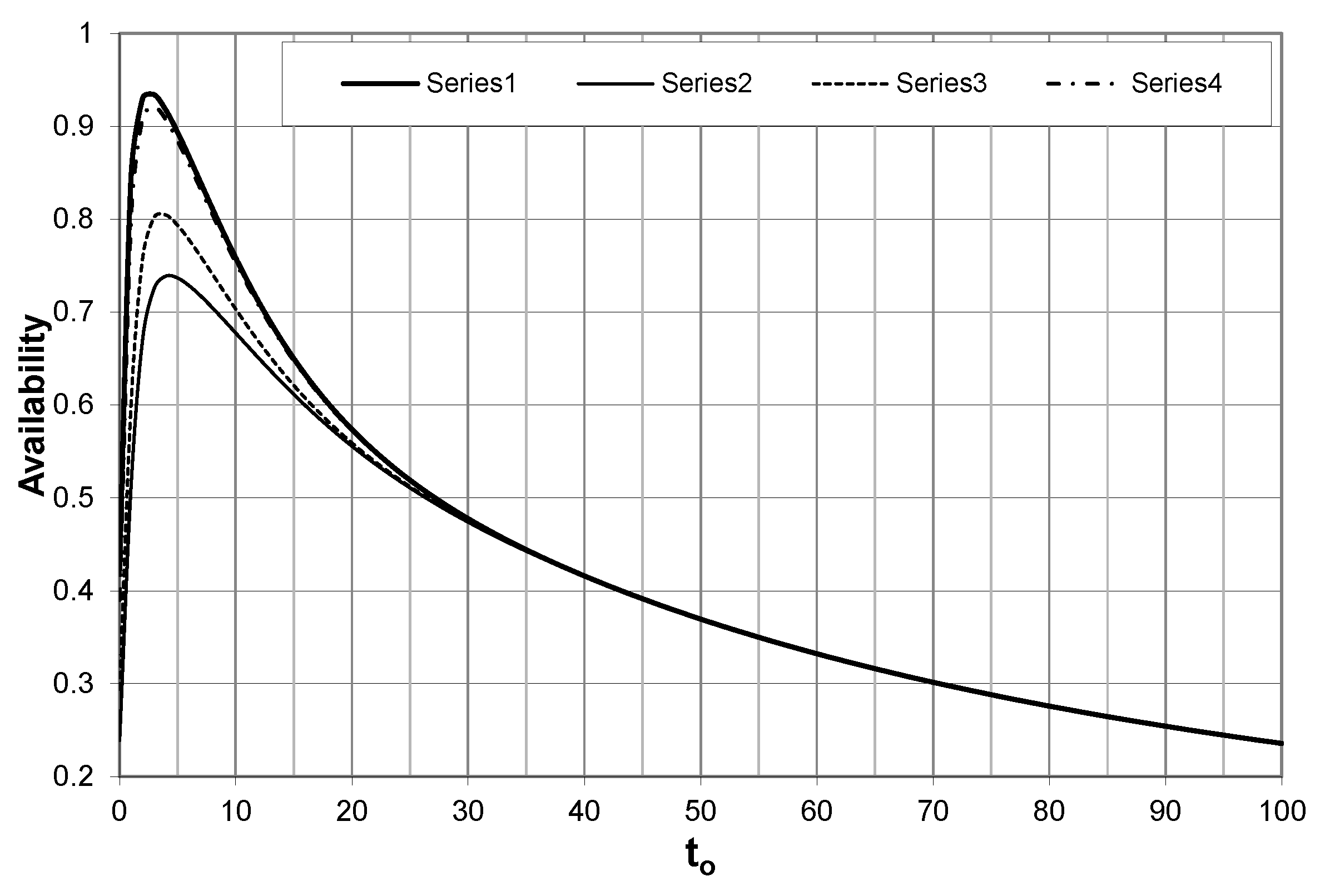
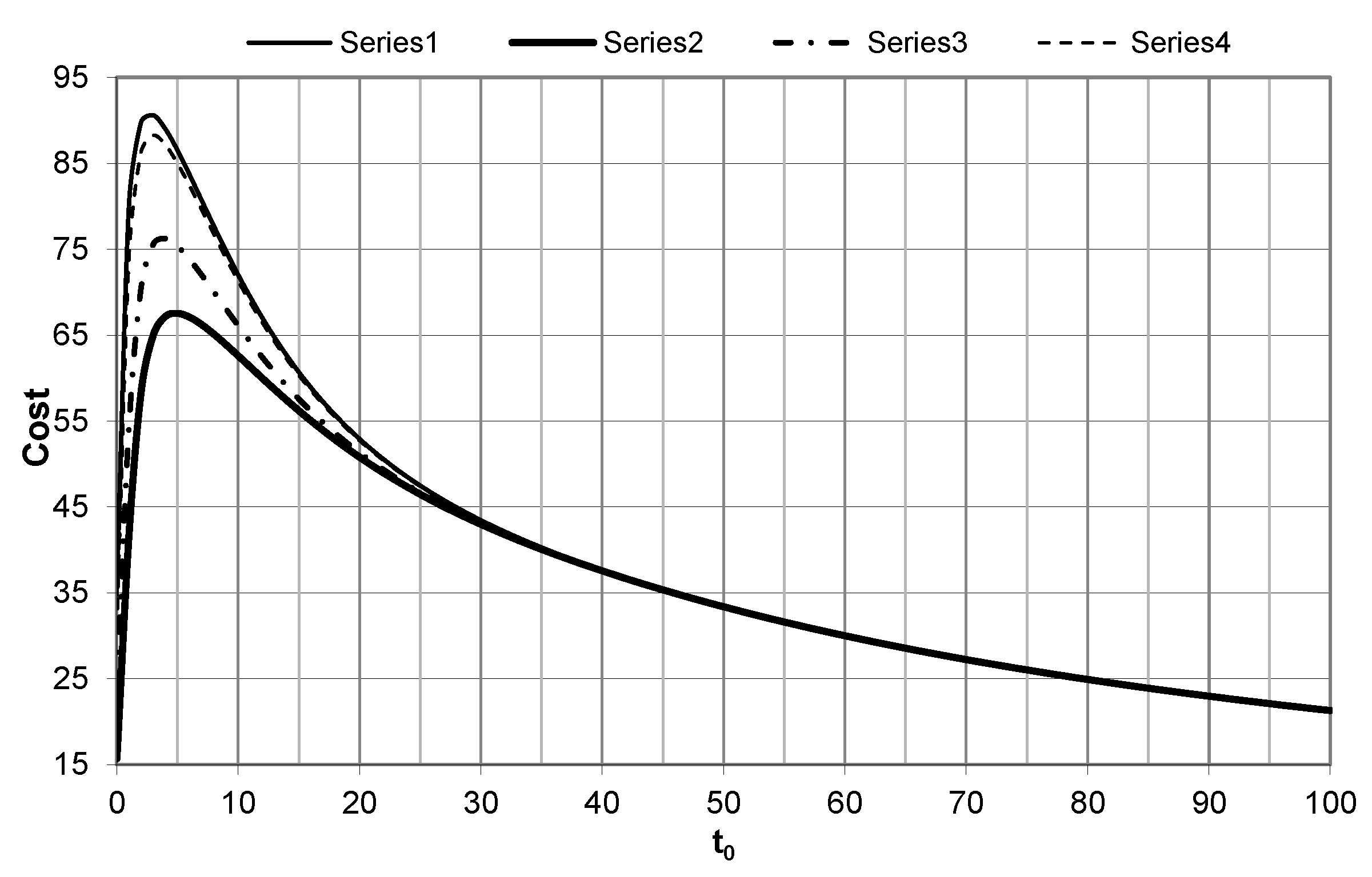
8. Numerical Illustration

In order to demonstrate the usefulness of the proposed system, we investigate the effect of PM and the other parameters on the reliability measures through the following numerical illustrations below. By setting $\alpha =100,k_1=30,k_2=10,k_3=20,k_4=10$ and

$$\begin{array}{ccc}& F_{\ell }\left(t\right)=& 1-(1+{\lambda }_{\ell }t)e^{-{\lambda }_{\ell }t},{\lambda }_{\ell }>0,\ell =1,2,3,4,\hfill \\ & G\left(t\right)=& 1-e^{-\nu t},\hfill \\ & B_{\ell }\left(t\right)=& 1-e^{-{\alpha }_{\ell }t},\ell =1,2.\hfill \end{array}$$

Figure 2, Figure 3 and Figure 4 show the effect of PM on the system reliability measures starting from time $t_0$ for some different choices of the system parameters, as shown below.

Series	p	${\lambda }_1$	${\lambda }_2$	${\alpha }_1$	${\alpha }_2$	$\beta$	${\lambda }_3$	${\lambda }_4$	$\delta$
1	0.3	0.1	0.05	1.5	2.5	0.2	0.3	0.5	1
2	0.3	0.1	0.05	0.2	2.5	0.2	0.3	0.5	1
3	0.3	0.1	0.05	1.5	0.5	0.2	0.3	0.5	1
4	0.8	0.1	0.005	1.5	2.5	0.2	0.3	0.5	1

From the figures, we see the system reliability measures increase from time $t_0$ to reach their maximum values and then decrease to the steady-state level (the values of system reliability measures without PM). This enables us to select the optimal period of time to perform PM.

Table 1. MTSF without PM at the starting time (ST) and the optimal time (OT) of $t_0$ with the corresponding optimal value of MTSF ($t_0$) (OV) to perform PM when $\nu =0.5$, $\delta =1$, ${\lambda }_3=0.3$, ${\lambda }_4=0.5$.

${\mathit{\alpha }}_1$	${\mathit{\alpha }}_2$	${\mathit{\lambda }}_1$	${\mathit{\lambda }}_2$	MTSF	ST		OT		OV
					$\mathit{p}=\mathbf{0.3}$	$\mathit{p}=\mathbf{0.8}$	$\mathit{p}=\mathbf{0.3}$	$\mathit{p}=\mathbf{0.8}$	$\mathit{p}=\mathbf{0.3}$	$\mathit{p}=\mathbf{0.8}$
1.5	2.5	0.01	0.001	403.38	17.5	27.9	54.3	73.0	611.31	532.27
			0.01	256.30	10.4	16.4	35.1	45.7	419.90	361.60
			0.05	80.20	3.0	4.8	10.1	13.3	125.40	108.80
		0.05	0.001	96.20	3.4	5.3	9.1	12.2	149.10	124.7
			0.01	91.31	3.1	4.9	8.8	11.7	145.40	121.51
			0.05	60.30	2.0	3.1	6.5	8.3	101.80	86.11
		0.10	0.001	57.06	1.8	2.7	5.2	6.4	98.90	81.70
			0.01	56.14	1.7	2.6	5.2	6.3	97.93	81.01
			0.05	46.42	1.4	2.2	4.6	5.7	82.53	69.20
	3.0	0.01	0.001	403.38	14.7	26.9	48.9	71.1	646.95	537.72
			0.01	256.30	8.8	15.9	31.8	44.9	444.78	365.25
			0.05	80.20	2.5	4.6	9.0	13.0	132.85	109.82
		0.05	0.001	96.20	2.9	5.1	8.3	13.9	160.69	126.19
			0.01	91.31	2.7	4.8	8.1	11.5	156.62	122.94
			0.05	60.30	1.7	3.1	6.0	8.1	108.86	87.08
		0.10	0.001	57.06	1.5	2.6	4.9	6.3	106.68	82.77
			0.01	56.14	1.5	2.5	4.8	6.2	105.65	82.05
			0.05	46.42	1.2	2.1	4.3	5.6	88.51	70.03
2.0	2.5	0.01	0.001	403.38	13.8	17.0	47.2	53.6	659.96	615.37
			0.01	256.30	8.3	10.2	30.8	34.7	454.27	421.93
			0.05	80.20	2.4	2.9	8.7	9.8	135.77	126.34
		0.05	0.001	96.20	2.7	3.3	8.0	8.9	166.48	151.46
			0.01	91.31	2.5	3.1	7.8	8.7	162.24	147.65
			0.05	60.30	1.6	2.0	5.8	6.5	112.32	103.24
		0.10	0.001	57.06	1.4	1.7	4.7	5.2	112.09	101.68
			0.01	56.14	1.5	1.7	4.7	5.1	110.99	100.72
			0.05	46.42	1.1	1.3	4.2	4.6	92.46	84.58
	3.0	0.01	0.001	403.38	11.2	16.3	41.8	52.1	709.81	625.0
			0.01	256.30	6.8	9.0	27.4	33.7	490.39	428.91
			0.05	80.20	1.9	2.8	7.7	9.6	146.26	123.36
		0.05	0.001	96.20	2.2	3.1	7.2	8.7	183.76	154.64
			0.01	91.31	2.1	3.0	7.1	8.5	178.97	150.74
			0.05	60.30	1.3	1.9	5.3	6.3	122.45	105.18
		0.10	0.001	57.06	1.4	1.6	4.4	5.1	123.92	103.89
			0.01	56.14	1.5	1.6	4.4	5.0	122.63	102.90
			0.05	46.42	0.9	1.3	3.9	4.5	101.25	86.23

and

Table 2. The optimal time (OT) and optimal value (OV) of the availability and cost function of the system in the steady state when $\nu =0.5,\delta =1,{\lambda }_3=0.3,{\lambda }_4=0.5$.

${\mathit{\alpha }}_1$	${\mathit{\alpha }}_2$	${\mathit{\lambda }}_1$	${\mathit{\lambda }}_2$	AV (${\mathit{t}}_0$)				Cost (${\mathit{t}}_0$)
				$\mathit{p}=\mathbf{0.3}$		$\mathit{p}=\mathbf{0.8}$		$\mathit{p}=\mathbf{0.3}$		$\mathit{p}=\mathbf{0.8}$
				OT	OV	OT	OV	OT	OV	OT	OV
1.5	2.5	0.01	0.001	7.0	0.9641	7.0	0.9488	8.2	95.47	9.3	93.42
			0.01	6.2	0.9627	6.4	0.9475	7.0	95.18	7.8	93.09
			0.05	3.8	0.9435	4.1	0.9287	3.9	92.16	4.4	89.84
		0.05	0.001	4.0	0.9542	4.2	0.9395	4.2	93.67	4.6	91.37
			0.01	3.9	0.9537	4.1	0.9390	4.1	93.57	4.5	91.27
			0.05	3.3	0.9413	3.5	0.9267	3.4	91.67	3.7	89.26
		0.10	0.001	2.9	0.9486	3.0	0.9301	3.0	92.06	3.3	89.59
			0.01	2.9	0.9443	3.0	0.9298	3.0	92.00	3.3	89.53
			0.05	2.5	0.9363	2.7	0.9218	2.7	90.76	3.0	88.23
	3.0	0.01	0.001	7.2	0.9684	7.1	0.9500	8.1	95.97	9.3	93.57
			0.01	6.2	0.9671	6.4	0.9487	6.9	95.68	7.8	93.22
			0.05	3.8	0.9437	4.1	0.9298	4.0	92.67	4.3	89.97
		0.05	0.001	3.9	0.9585	4.2	0.9406	4.1	94.17	4.6	91.50
			0.01	3.8	0.9580	4.2	0.9401	4.1	94.07	4.5	91.39
			0.05	3.2	0.9455	3.4	0.9278	3.3	92.18	3.7	89.38
		0.10	0.001	2.8	0.9487	3.0	0.9311	2.9	92.57	3.3	89.71
			0.01	2.7	0.9483	3.0	0.9308	2.9	92.52	3.4	89.63
			0.05	2.5	0.9406	2.7	0.9228	2.6	91.27	3.0	88.34
2.0	2.5	0.01	0.001	7.3	0.9702	7.1	0.9649	7.9	96.21	8.7	95.33
			0.01	7.1	0.9703	6.1	0.9636	7.9	96.21	7.4	95.00
			0.05	3.8	0.9488	3.9	0.9444	3.9	92.98	4.2	91.84
		0.05	0.001	3.9	0.9608	4.0	0.9554	4.1	94.51	4.3	93.39
			0.01	3.9	0.9602	3.9	0.9549	4.0	94.42	4.2	93.29
			0.05	3.2	0.9479	3.2	0.9426	3.3	92.55	3.4	92.32
		0.10	0.001	2.7	0.9518	2.9	0.9461	2.9	93.03	3.1	91.73
			0.01	2.7	0.9515	2.8	0.9460	2.9	92.97	3.0	91.67
			0.05	2.5	0.9435	2.6	0.9380	2.6	91.73	2.7	90.37
	3.0	0.01	0.001	6.8	0.9749	7.0	0.9662	7.8	96.72	7.8	95.45
			0.01	6.8	0.9734	6.3	0.9648	6.7	96.44	7.3	95.15
			0.05	3.7	0.9543	3.9	0.9456	3.8	93.52	4.1	91.98
		0.05	0.001	3.8	0.9652	4.0	0.9566	4.0	95.04	4.3	93.53
			0.01	3.7	0.9648	4.0	0.9536	3.9	94.95	4.2	93.43
			0.05	3.0	0.9525	3.2	0.3938	3.2	93.1	3.4	91.46
		0.10	0.001	2.7	0.9564	2.8	0.9475	3.0	93.54	3.0	91.87
			0.01	2.7	0.9561	2.8	0.9474	2.8	93.53	3.0	91.81
			0.05	2.4	0.9481	2.5	0.9392	2.5	92.30	2.7	90.52

display the system reliability measures for some other choices of parameters. From the numerical results displayed in the graphs and Table 1 and Table 2, one can observe the following:

(i)

The reliability measures of the system increase (decrease) as failure rate parameters decrease (increase).

(ii)

The reliability measures of the system increase (decrease) as the rates of the repair rates increase (decrease).

(iii)

The reliability measures of the system increase (decrease) as the PM rates increase (decrease).

(iv)

PM does not appear to be useful when the parameters of the failure rates are large or small (for example, when ${\lambda }_1=1$ and ${\lambda }_2=2$, the optimal time for PM is not approached).

(v)

For the large values of $t_0$, the reliability measures of the system reach the stable stage; this means that PM is not useful.

(vi)

The starting point and the optimal times of PM decrease as the failure parameters increase. Moreover, the time interval between the starting and optimal times of PM decreases as the parameters of the failure rate increase.

9. Conclusions

In this paper, the effect of preventive maintenance on reliability measures of the propped system consisting of one priority unit and one ordinary unit is investigated in terms of the mean time to first system failure, availability, and cost function. The priority unit has normal, total, and partial failures, while the ordinary unit has two modes: normal and total failure. If the priority unit is in normal mode until time t without total (or partial) failures, then it should go to PM (costlier with probability p and cheaper with probability $(1-p)$) provided that the standby unit is available. The switchover is perfect and instantaneous, and only one server operator is available for both of the repairs and PM.

The configurations and states of the system are descried, and the transitions probabilities between the different states and the corresponding mean sojourn times are calculated. Next, the Laplace transforms and transition probabilities are utilized to derive the closed form of the mean time to system failure as one of the reliability measures of the system. In addition, the steady-state availability of the proposed system is investigated through some recursive relations. The expected busy period of the system with both repair and PM is derived. To demonstrate the effect of PM on the system reliability, cost–benefit analysis is carried out.

Some numerical illustrations are displayed to show the usefulness of the findings of the paper based on certain choices of the system parameters. Theses illustrations show the importance of parameter selections in increasing the efficiency of systems and in determining the optimal time interval to start PM. Finally, we conclude from the findings that the choices of system parameters and the type of PM should be taken into account for the configurations of new systems.

References

1. El-Sherbeny, M.; AL-Hussaini, E.K. Characteristic reliability measures of mixed standby components and asymptotic estimation. Int. J. Stat. Appl. 2012, 2, 11–23. [Google Scholar] [CrossRef]
2. Kumar, A.; Malik, S.C. Stochastic modeling of a computer system with priority to PM over S/W replacement subject to maximum operation and repair times. Int. J. Comput. Appl. 2012, 43, 27–34. [Google Scholar] [CrossRef]
3. Sharma, K.S.; Sharama, D.; Sharama, V. Reliability measures for a system having two-dissimilar cold standby units with random check and priority repair. Res. Math. Stat. 2010, 2, 69–74. [Google Scholar]
4. Yusuf, I.; Bala, S.; Ali, U.A. Stochastic modeling of a non maintained system with two stages of deterioration. Int. J. Basic Appl. Sci. 2012, 1, 314–320. [Google Scholar] [CrossRef] [Green Version]
5. Yuan, L.; Meng, X. Reliability analysis of a warm standby repairable system with priority use. Appl. Math. 2011, 35, 4295–4303. [Google Scholar] [CrossRef]
6. El-Said, K. Stochastic analysis of a two-unit cold standby system with two-stage repair and waiting time. Sankhya 2010, 72, 1–10. [Google Scholar] [CrossRef]
7. Mahmoud, M.A.W.; Moshref, M.E. On a two-unit cold standby system considering hardware, human error failures and preventive maintenance. Math. Comput. Model. 2010, 51, 736–745. [Google Scholar] [CrossRef]
8. Mahmoud, M.A.W.; Mohie El-Din, M.M.; El-Said Moshref, M. Optimum preventive maintenance for a 2-unit priority-standby system with patience-time for repair. Optimization 1994, 29, 361–379. [Google Scholar] [CrossRef]
9. Di Nardo, M.; Madonna, M.; Murino, T.; Castagna, F. Modelling a safety management system using system dynamics at the Bhopal incident. Appl. Sci. 2020, 10, 903. [Google Scholar] [CrossRef] [Green Version]
10. Wells, C.E. Reliability analysis of a single warm-standby system subject to repairable and nonrepairable failures. Eur. J. Oper. Res. 2014, 335, 180–186. [Google Scholar] [CrossRef]
11. Zhong, C.; Jin, H. A novel optimal preventive maintenance policy for a cold standby system based on semi-Markov theory. Eur. J. Oper. Res. 2014, 332, 405–411. [Google Scholar] [CrossRef]
12. Levitin, G.; Finkelstein, M.; Dai, Y. Optimal preventive replacement policy for homogeneous cold standby systems with reusable elements. Reliab. Eng. Syst. Saf. 2020, 204, 107135. [Google Scholar] [CrossRef]
13. Ruiz-Castroa, J.E.; Dawabshab, M. A multi-state warm standby system with preventive maintenance, loss of units and an indeterminate multiple number of repairpersons. Comput. Ind. Eng. 2020, 142, 106348. [Google Scholar] [CrossRef]
14. Ge, X.; Sun, J.; Wu, Q. Reliability analysis for a cold standby system under stepwise Poisson shocks. J. Control Decis. 2021, 8, 27–40. [Google Scholar] [CrossRef]
15. Gao, S.; Wang, J. Reliability and availability analysis of a retrial system with mixed standbys and an unreliable repair facility. Reliab. Eng. Syst. Saf. 2021, 205, 107240. [Google Scholar] [CrossRef]
16. Kumar, A.; Barak, M.S.; Devi, K. Performance analysis of a redundant system with Weibull failure and repair laws. Rev. Investig. Oper. 2016, 37, 247–257. [Google Scholar]
17. Kumar, J.; Goel, M. Availability and profit analysis of a two-unit cold standby system for general distribution. Cogent Math. Stat. 2016, 3, 1262937. [Google Scholar] [CrossRef]
18. Hirata, R.; Arizono, I.; Takemoto, Y. On reliability analysis in priority standby redundant systems based on maximum entropy principle. Qual. Technol. Quant. Manag. 2021, 18, 117–133. [Google Scholar] [CrossRef]
19. Kumar, A. Cost–benefit analysis of a repairable system in abnormal environmental conditions. Palest. J. Math. 2016, 5, 111–119. [Google Scholar]
20. Kumar, P.; Chowdhary, S. Stochastic analysis of a two-unit standby system model with preventive maintenance and random appearance and disappearance of repairman. Math. Eng. Sci. Aerosp. 2015, 6, 221–231. [Google Scholar]
Figure 1. The Transitions diagram.
Applsci 11 03861 g001
Figure 2. The MTSF of the system based on different parameter values.
Applsci 11 03861 g002
Figure 3. The availability of the system based on different parameter values.
Applsci 11 03861 g003
Figure 4. The cost function based on different parameter values.
Applsci 11 03861 g004