Application of the SWAT-EFDC Linkage Model for Assessing Water Quality Management in an Estuarine Reservoir Separated by Levees

Abstract

Estuarine reservoirs are available for use in various water resource systems. In agriculture, supplying irrigation water that meets water quality standards is essential for food safety. This study focused on the Ganwol estuarine reservoir in the midwestern region of South Korea, which suffers from water quality deterioration problems. To explore the water quality improvement in an estuarine reservoir, it is essential to understand the characteristics of water quality changes in the reservoir following water pollution control management. Therefore, the purpose of this study is to evaluate the effects of water quality management on the estuarine reservoir, which is separated by levees, using the soil and water assessment tool (SWAT)-environmental fluid dynamics code (EFDC) linkage model. In this study, soil remediation by dredging the reservoir’s bottom soil and effluent control from public sewage treatment works were considered as the water management plans. The results of this study indicate that reducing the internal load of the reservoir increases internal resilience and reducing the external inflow load decreases the impact on the system. Hence, comprehensive measures are effective in improving water quality.

1. Introduction

An estuary refers to a point where the final outlet of a stream converges with the marine environment, and is a water body that combines fresh water and seawater [1]. This leads to the creation of a productive ecosystem [2], and acts as a natural runoff filter to improve water quality [3]. In addition, by artificially preventing marine circulation through seawall construction and creating an estuarine reservoir-closed water environment, estuaries supply water from diverse sources, and some areas use estuarine water resources as agricultural water [4,5].

Estuarine reservoirs are the final destination of upstream pollution sources when considering the geographical features of being situated in estuaries, and most estuarine reservoirs suffer from water quality pollution because of limited seawater circulation [6,7,8]. In particular, in the Ganwol estuarine reservoir, our study site, because of reclamation works, deposit atomization has resulted from tide speed decline [9], inflow of livestock wastewater and domestic wastewater as a point source pollution, and inflow of agricultural land outflow as a nonpoint source pollution [10]. This has led to the resupply of organic nutrients within the reservoir because of the resuspension of fine sediments and an increase in the phosphorous inner load [11]. The water quality of estuarine reservoirs is crucial for biodiversity, sustainability [12], and the production of high-quality, eco-friendly agricultural products on reclaimed lands [13]. Therefore, to improve the eco-friendly characteristics of estuarine reservoirs and reclaimed lands, it is important to develop water quality management measures based on a comprehensive understanding of the upstream estuarine reservoirs, inflowing pollutants, and estuarine reservoir water body features.

When analyzing estuarine reservoir watersheds and water environment changes based on water quality pollution management measures, applying actual methods and conducting various assessments are useful for improving accuracy and reducing the uncertainty of data. However, there are limitations in terms of finance and time. Additionally, there is a lack of data on the flow and water quality of all streams flowing into estuarine reservoirs or on their water levels and water quality changes. Therefore, modeling is generally used to examine various scenarios. As estuarine reservoirs encompass watersheds and reservoirs, it is necessary to develop three-dimensional watershed models, hydrological models, and water bodies within estuarine reservoir models. To create a linkage model, a watershed model is the boundary condition for the hydrodynamic and water quality model of a three-dimensional numerical model, and internal and external linkages are necessary [14]. Several studies have examined the linkage between watershed and reservoir models using the hydrological simulation program-Fortran (HSPF) model [15] and the environmental fluid dynamics code (EFDC) model [16], which has been used to simulate the watershed runoff and reservoir water quality of a river estuary [14] or a river-reservoir combined system [17]. The HSPF-EFDC linkage model has also been used to enhance the prediction accuracy of water quality in rivers using the ensemble Kalman filter (EnKF) technique [18,19].

Although the HSPF-EFDC linkage model has the advantage of being able to easily import the HSPF input file through the linkage file, this study evaluates the water quality improvement scenarios by linking the soil and water assessment tool (SWAT) [20] and EFDC models. The SWAT model has been widely used in studies on the upstream nonpoint source pollution of agricultural systems [21,22,23,24,25,26]. In particular, [25] reviewed several studies and concluded the following: the SWAT model applied in various countries performs well in nonpoint source pollution simulation. The sediment simulation capability is also important in the simulation of nonpoint source pollution. [27] suggested that the simulation capability of the SWAT model is slightly better than that of the HSPF model. Recently, the SWAT model has been linked with the EFDC model to simulate the upstream inflow and water quality in lakes or reservoirs [28,29], and [29] pointed out that the SWAT-EFDC linkage model could be a useful tool for simulating water quality management scenarios and for applying the best management practices (BMPs) on a watershed scale. Therefore, this study evaluates the water quality improvement scenarios by linking the SWAT and EFDC models to consider the agricultural system and nonpoint source pollution of the upper watershed.

The measures to resolve the water quality issues of estuarine reservoirs are mainly divided into watershed measures to reduce the external pollution load flowing into estuarine reservoirs and estuarine reservoir measures to reduce the internal occurrence load. There are two options for water quality management of watersheds: point source and nonpoint source pollution. A representative measure of point source pollution management is the quality management of discharged water from public sewage treatment works (PSTWs) for downstream reservoirs [30]. In the case of nonpoint source pollution related to estuaries or estuarine reservoirs, studies have mainly considered BMPs [31,32,33] and artificial wetlands [34,35] to reduce the inflow of nonpoint source pollution from the upper watersheds. Water quality management measures within estuarine reservoirs include internal development, lake water management, seawater circulation, and dredging within estuarine reservoirs. Thus, this study simulates the measures for water quality improvement and assesses the results after considering low-quality soil improvement (internal factor) and inflow of the PSTW effluent (external factor).

A list of acronyms and abbreviations used throughout this article in given

Table 1. Description of abbreviations used throughout the article.

Abbreviations	Expanded Form or Meaning
SWAT	Soil and water assessment tool
EFDC	Environmental fluid dynamics code
HSPF	Hydrological simulation program-Fortran
PSTWs	Public sewage treatment works
BMP	Best management practices
EnKF	Ensemble Kalman filter
O/S	(observed average)/(simulated average)
Ave.	Average
cal.	Calibration
val.	Validation

.

Ganwol Reserovir, the study area, suffers from point source water pollution from PSTWs located at the end of the upper watershed and nonpoint source pollution from the surrounding agricultural land. In addition, because the upstream and downstream of the estuarine reservoir are separated by levees, which have three small waterways, it is necessary to examine whether improving the water quality upstream can be spread throughout the reserovir. It is difficult to provide a simple interpretation of the effects resulting from water quality improvement techniques for estuarine reservoirs with sophisticated geographical features. Therefore, this study aims to analyze the annual average water quality concentrations and T-P reduction efficiency, and assess the water quality management of estuarine reservoirs using the SWAT-EFDC linkage model.

2. Materials and Methods

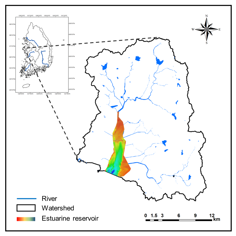
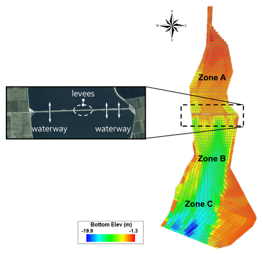
2.1. Study Area and Bottom Soil Characteristics of the Estuarine Reservoir

The study site, the Ganwol estuarine reservoir located in the midwestern part of South Korea (Figure 1), was established in 1995. The total watershed area, agricultural water supply area, and maximum water surface area were 48,770 ha, 6446 ha, and 2504 ha, respectively. In the watershed area, 39.6 % were rice paddies, 30.3 % were forests and fields, 15.4 % were farms, 8.8 % were others, and 5.9 % were water surfaces. Runoff and water quality measurement points existed in four streams within the study site, and data were collected once a month from 2011–2018. Moreover, we collected the daily outflow and water quality data of the PSTWs and livestock manure processing facilities within the watershed. They have been used as point source pollution input data in the model.

To investigate the bottom soil characteristics, a soil sampling was performed using a grab sampler at three locations in the Ganwol estuarine reservoir. A physicochemical analysis of sediments was performed using ignition loss, organic matter content, T-N, T-P, Cd, Cu, Pb, As, Cr6+, and sieve analysis.

Table 2. Bottom soil characteristics of the Ganwol estuarine reservoir.

Sampling Date	Content	Ignition Loss (%)	Organic Matter (%)	T-N (%)	T-P (mg/kg)
24 May 2018	Zone A	3.7	2.10	0.154	607.46
	Zone B	0.8	0.50	0.058	448.03
	Zone C	0.9	0.25	0.042	385.88
13 July 2018	Zone A	2.1	1.20	0.081	450.03
	Zone B	0.6	0.99	0.073	417.13
	Zone C	0.4	1.36	0.102	409.50

shows the results of the sediment contamination analysis. According to the analysis results, the values in Zone A were higher than those in Zone B and Zone C for all ignition losses, T-N, and T-P.

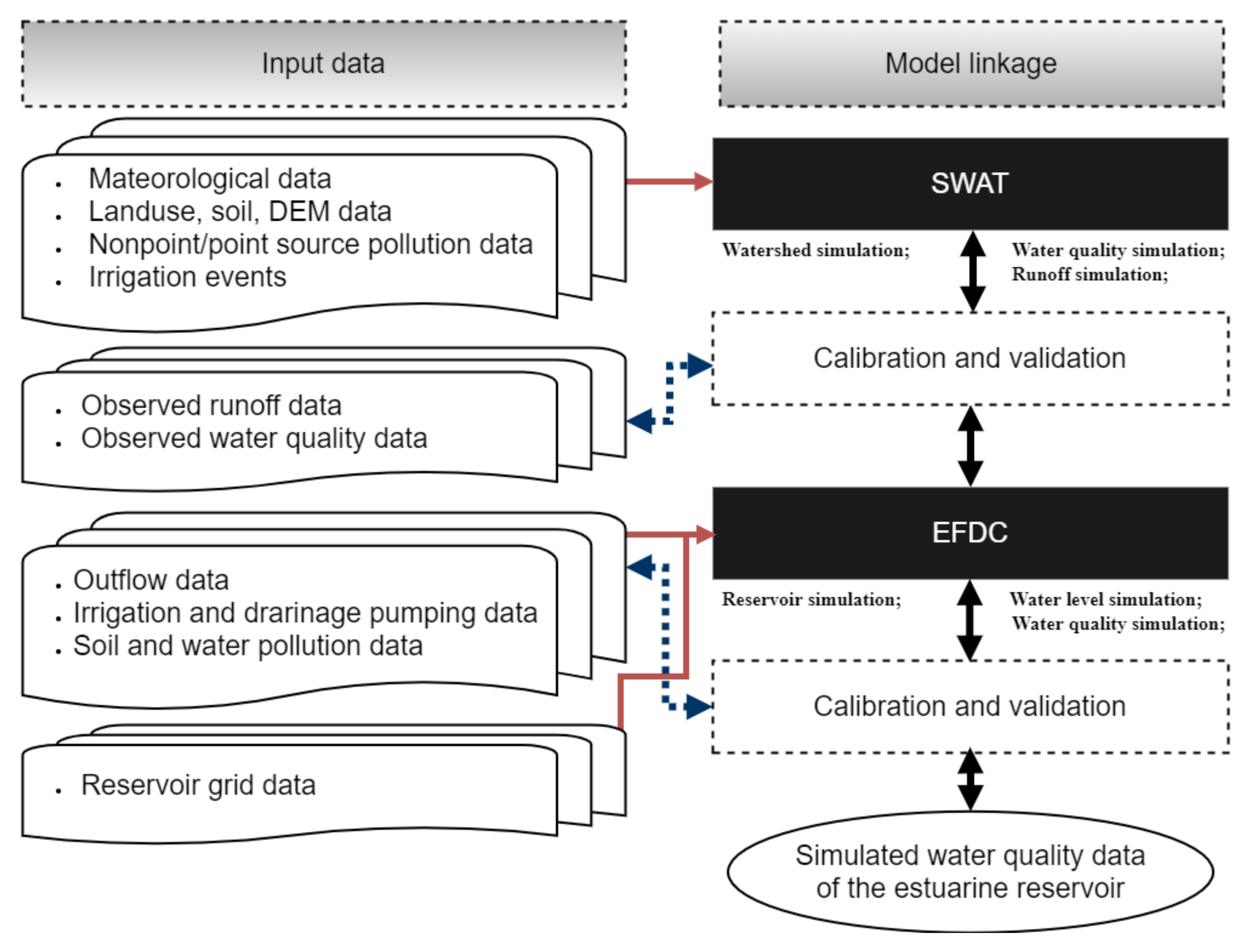
2.2. SWAT-EFDC Linkage Model

When analyzing the water quality changes of the corresponding estuarine reservoir measures, actual observations are desirable. However, because of time and cost constraints, assessing the corresponding measures using hydrological and reservoir water models is more efficient. In this study, we used the SWAT model as the watershed model and EFDC model as the reservoir model, and their effects were verified following their application to the watersheds in Korea [28,29]. Figure 2 shows the linkage between the output and input data of the watershed and reservoir models.

Calibration and validation were conducted using hydrological and water quality measurement values to enhance the reproducibility of water quality and inflow from the upstream estuarine reservoir watershed based on the SWAT model. The derived optimal calibration and validation results were used as inflow and water quality input data in the EFDC model. The parameters of the EFDC model were determined through meteorological data, inflow and outflow through pumping stations and sluice gates, soil pollution data, and measured data of the water quality pollution. Finally, water quality simulation results were derived using the EFDC model and their corresponding water quality management measures were used for assessing various scenarios in the upstream watershed and estuarine reservoir.

2.3. EFDC Model Setup

This study organized an EFDC model grid for the estuarine reservoir based on the measured data (Figure 3). The grid organization can be detailly performed based on the measured data. However, a stable simulation of the numerical analysis model is possible when the calculation grid has a square shape. Hence, an adequate grid size and number is necessary to reduce the simulation time. This study analyzed the adequacy of grid organization. The number of valid computational grids was 9359 in the horizontal direction, and the grids were arranged in five equidistant intervals in the vertical direction. The grid system used a rectangular coordinate system in the horizontal direction and a sigma coordinate system in the vertical direction. The sigma coordinate system has the advantage of setting a diverse layer thickness and preventing numerical errors with regard to domains undergoing drastic depth changes.

As for the EFDC model, calibration and validation were conducted from 2015–2017 using the water quality monitoring data from the Ministry of Environment. Temperature data were calibrated from 2015–2017, and the diverse parameters of the EFDC model were corrected in the order of DO, T-P, and PO₄-P. In the case of the EFDC model, water quality changes in the reservoir are influenced not only by the inflow pollutants but also seasonal effects, currents, and meteorological changes based on the internal reservoir system. Therefore, this study also considered T-N and Chl-a in the calibration and validation.

In addition, because the estuarine reservoir has levees in the middle and each zone has a different environment, it was divided into three zones to organize the EFDC model parameters corresponding to each zone (Figure 3).

Finally, we conducted water quality calibration and validation with regard to Zones A and B. The objective function used O/S, that is, the value of (observed average)/(simulated average). The accuracy of the model increases as the O/S values approaches 1.

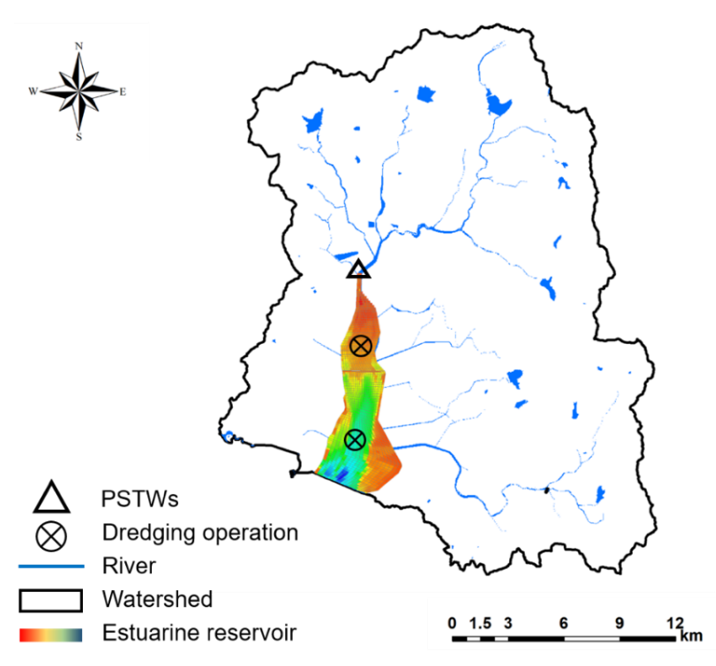
2.4. Scenario Description

In this study, a total of eight scenarios were considered, and

Table 3. Description of the applied scenario in this study.

Scenario	Content
No scenario	Scenario 0 (Now)
Group A: Dredging operation in Zone A	Scenario 1 (P and N leaching rate 60% reduction)
	Scenario 2 (P and N leaching rate 80% reduction)
Group B: Dredging operation in Zones A and B	Scenario 3 (with Scenario 3) (P and N leaching rate 40% reduction in Zone B)
	Scenario 4 (with Scenario 4) (P and N leaching rate 40% reduction in Zone B)
Group C: Effluent control from PSTWs	Scenario 5 (50% T-P effluent reduction)
	Scenario 6 (90% T-P effluent reduction)
Group D: Combined scenario	Scenario 7 (Scenario 4 and Scenario 5)
	Scenario 8 (Scenario 4 and Scenario 6)

summarizes them. First, as shown in Figure 4, Group A considered the dredging scenario in Zone A, which is currently underway, for low-quality bottom soil remediation. Zone A and Zone B were the same estuary area in the past, and the benthic rate of Zone A was three times that of Zone B; thus, a reduction of up to 80 % was considered. Second, bottom soil remediations of Zones A and B were considered together. Third, regarding the effluent control of PSTWs, Group C considered the facility of the PSTW extension (T-P reduction 50 %), and a new facility construction for an advanced phosphorus treatment (T-P reduction 90 %). Finally, rather than considering the scenarios of soil remediation for each zone and applying the effluent control from the PSTWs separately, a simulation was conducted after considering various combinations of the scenarios (Group D).

3. Results

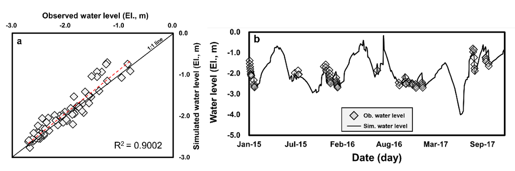
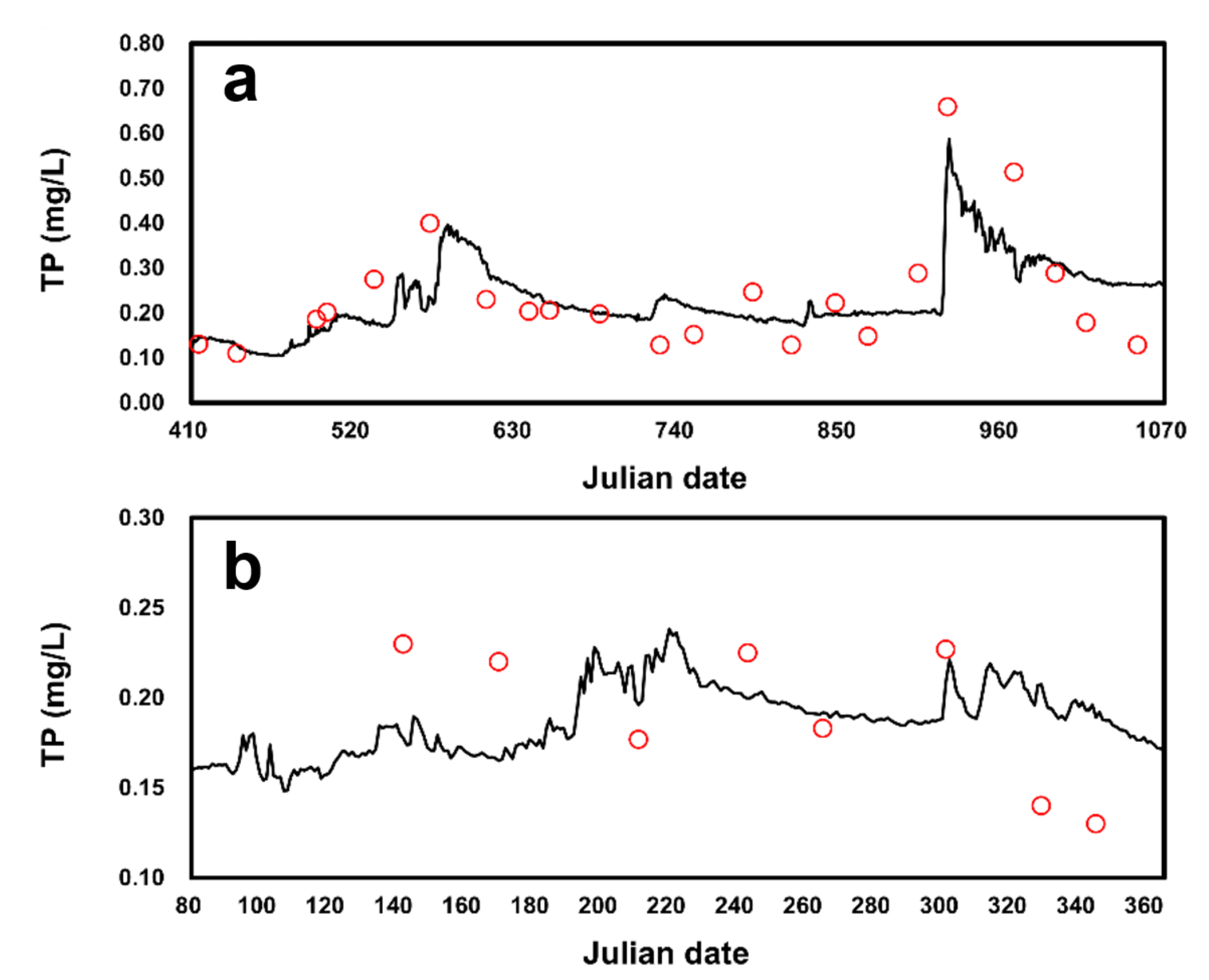
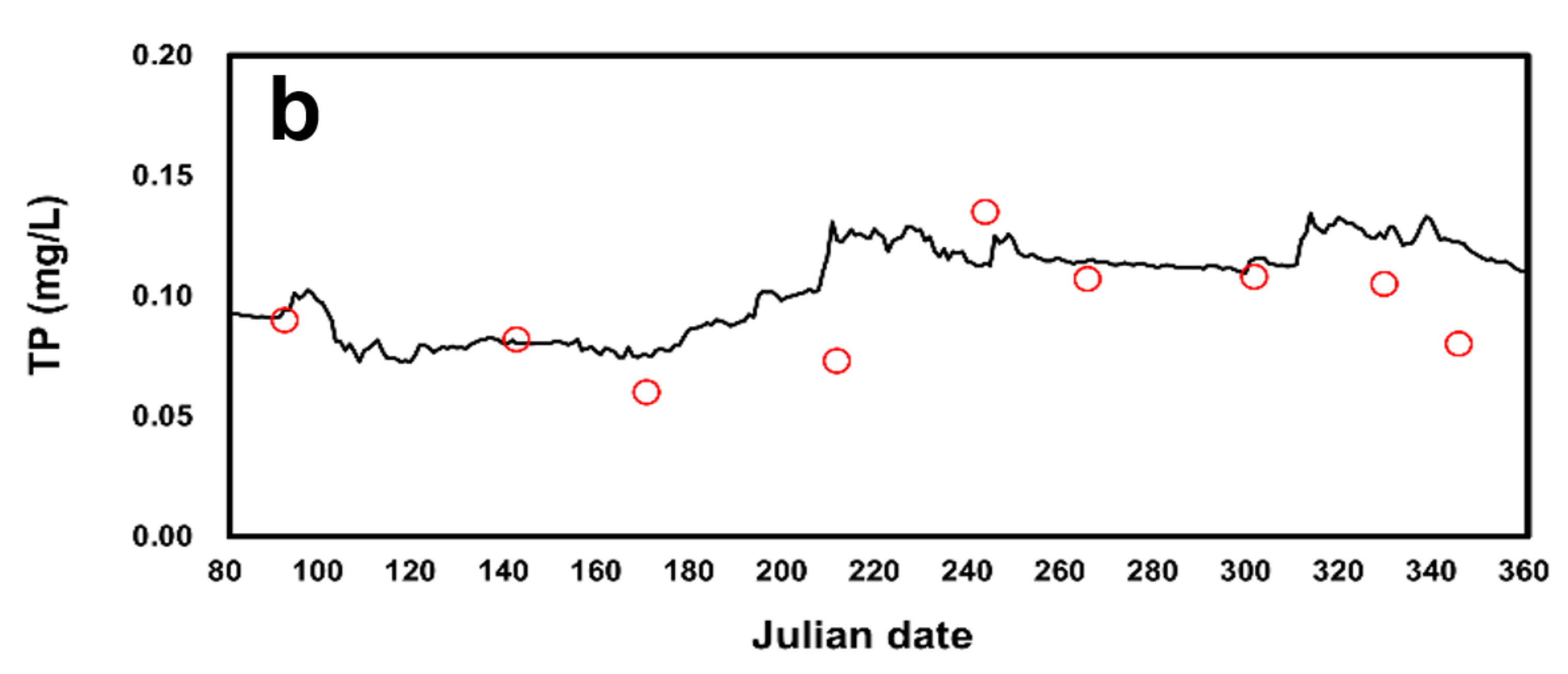
3.1. Model Calibration and Validation Results

In this study, we used the SWAT model for watershed inflow and water quality simulations, and the results of [6] for calibration and validation. The drainage sluice gate operation log and pumping station data of the irrigation and drain facilities were used for the water level simulation of the estuarine reservoir using the EFDC model from 2015–2017. As a calibration result of the water levels, the R-squared value (R² = 0.9002) shows good results and a high reproducibility (Figure 5).

In this study, observed water quality data from 2016–2017 were used for calibration, and those from 2015 were used for validation. For 2015, the observed values were used for validation from day 81 onward after considering the influence of the model’s initial value. In particular, as there is a strong influence of algae behavior during the water quality simulation using the EFDC model, other water quality data (Chl-a, T-N, etc.) have been used in T-P calibration after referring to the measured values. Following the calibration and validation (Figure 6 and Figure 7), the calibration values of the two points were higher than 0.95; thus, the calibration was performed well (

Table 4. Calibration and validation results of EFDC model simulation.

Location	Content	TEMP	DO	T-P (cal.) (2016–2017)	T-P (val.) (2015)
Zone A-observation point	Observed Ave.	16.64	10.34	0.242	0.201
	Simulated Ave.	17.17	10.41	0.232	0.186
	O/S	0.969	0.993	0.957	0.927
Zone B-observation point	Observed Ave.	16.60	11.99	0.143	0.105
	Simulated Ave.	17.32	10.62	0.148	0.101
	O/S	0.959	1.128	0.964	0.961

).

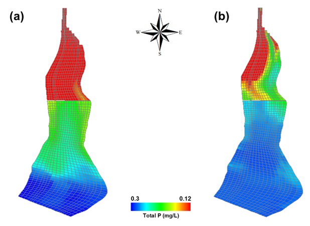
3.2. Reservoir Simulation Result

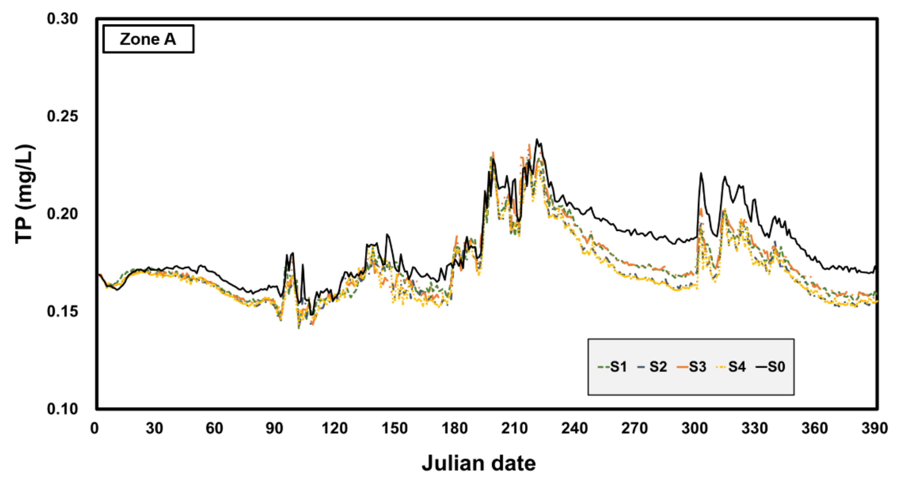
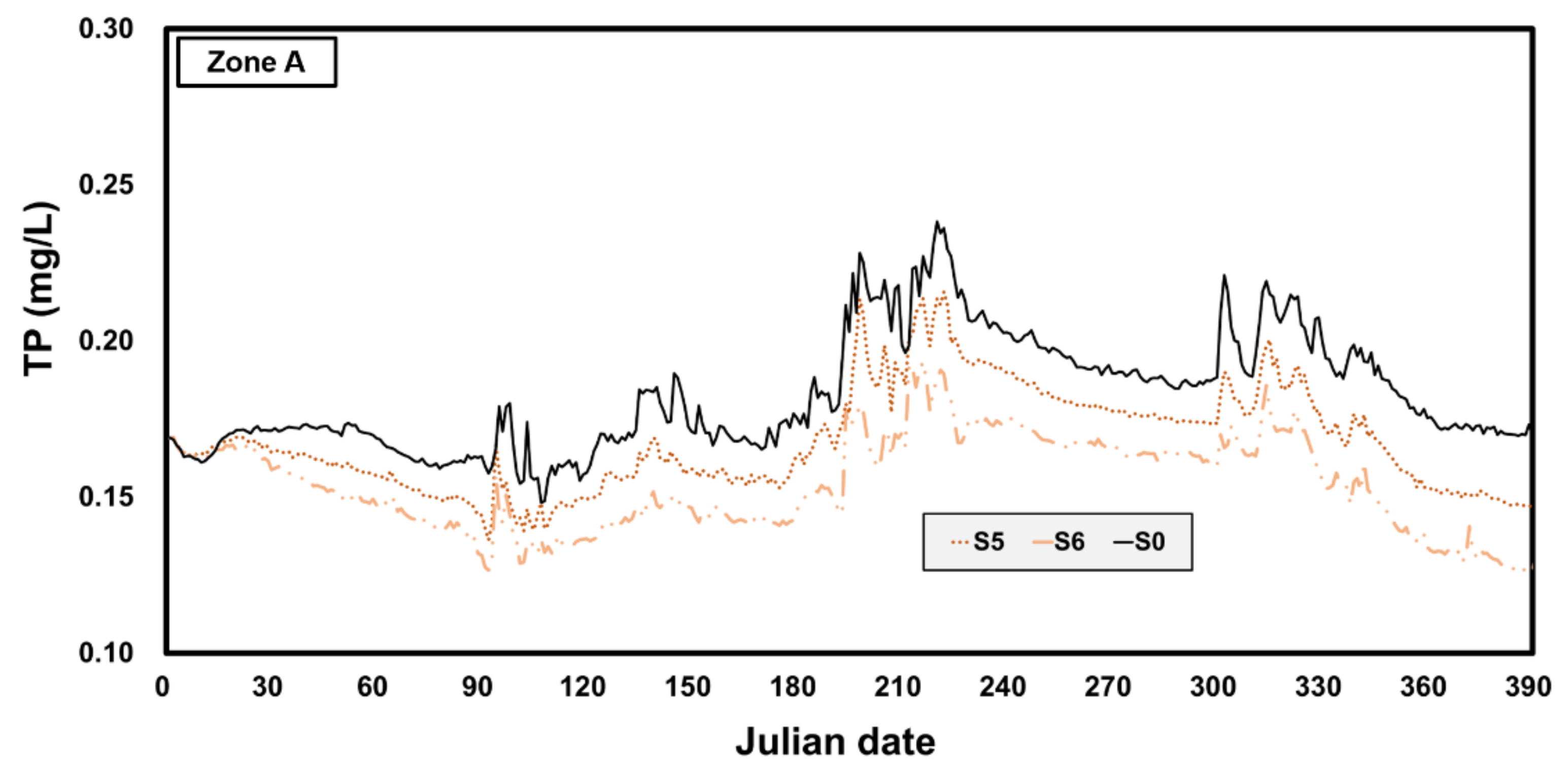
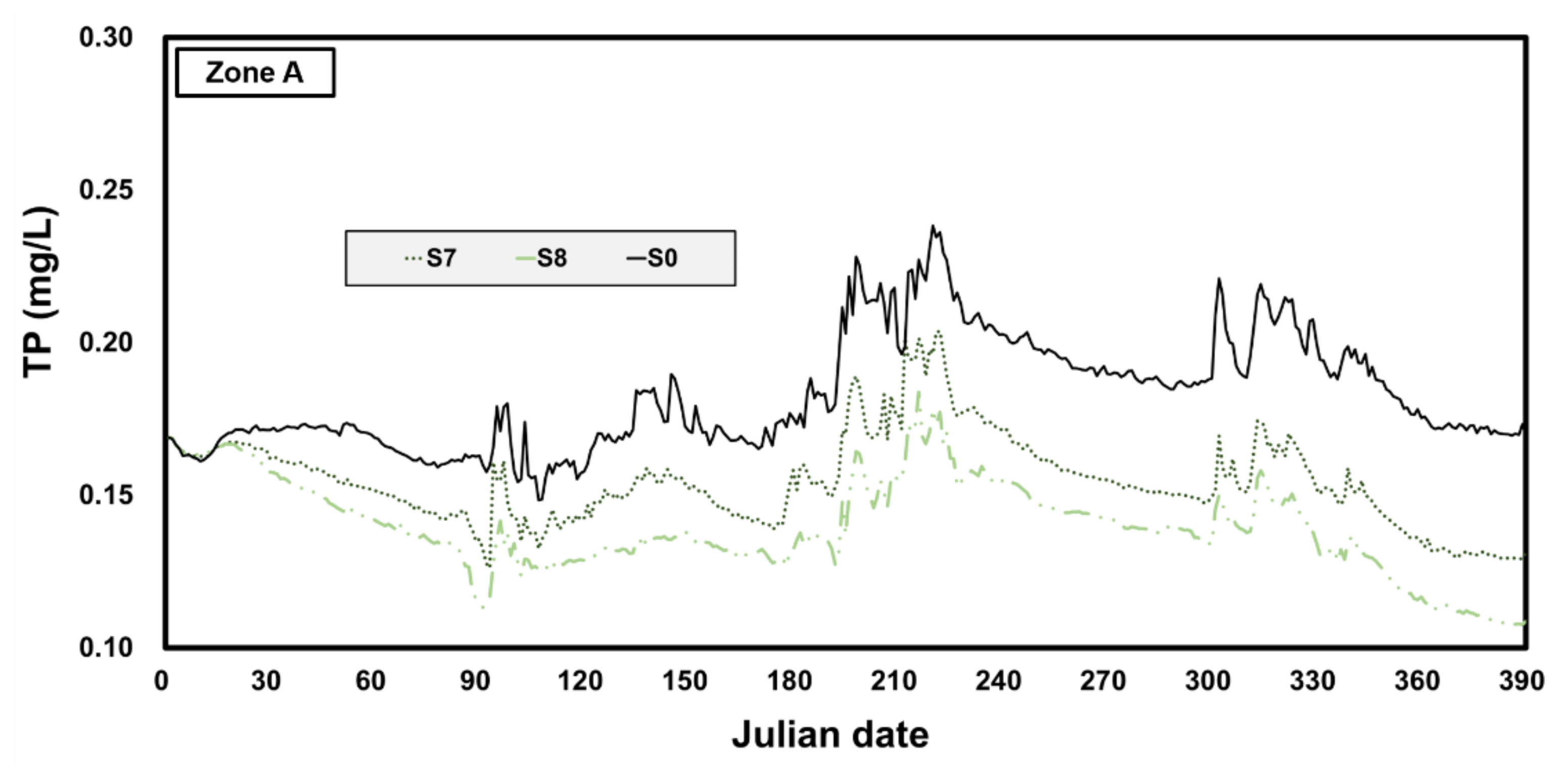
3.2.1. Zone A Simulation Results

Figure 8 shows the simulation results of the T-P water quality changes with respect to Zone A in 2015 for the reservoir. As for the annual average water quality, T-P is 0.183 mg/L when no measure is applied, and the following results are obtained when the scenario is applied: S1, 0.175 mg/L; S2, 0.172 mg/L; S3, 0.175 mg/L; and S4, 0.171 mg/L. When conducting dredging only with regard to Zone A, in 2015, the target water quality standard of 1 mg/L was not satisfied. As for the overall water quality change tendencies, the slope is gradual when no measure is applied during the water quality deterioration process. This implies the water quality resilience of the estuarine reservoir is low when the load is high within the reservoir. Thus, it is difficult to accomplish the water quality objective of an estuarine reservoir merely by dredging. However, this measure can increase the resilience of estuarine reservoir systems.

As a result of the simulation in Scenario 5, in which dredging was conducted in Zone B based on Scenario 3, and comparing the results with corresponding scenarios, it is found that a thorough circulation of the water quality does not happen upstream and downstream because of the influence of the embankment placed in the middle. Even if dredging takes place in Zone B, it cannot significantly influence the upstream water quality changes. The annual average water quality was slightly lower than that in the case where no measure was applied (T-P value 0.183 mg/L). However, the T-P water quality concentration in scenario 5 has an annual average value of 0.175 mg/L, which is similar to that of S3.

As a result of the simulation in Scenario 7, which conducts dredging in Zone B based on Scenario 4 (unlike Scenario 5 in a state where Zone A dredging progresses to a significant degree), the water quality is partially influenced by Zone B dredging. Regarding the actual annual average water quality concentration, when compared with the T-P simulation result of 0.172 mg/L in S4, the T-P simulation result of Scenario 7 was 0.171 mg/L. When considering not only the average concentration but also the water quality change tendency, unlike in the beginning of 2015, the water quality concentration is low at the point where water quality is aggravated over time. This implies a minor increase in resilience than the previous scenario.

Figure 9 shows the simulation results of the water quality changes with regard to the cases of extending the phosphorus treatment facility at a PSTW located at the reservoir inlet (Scenario 5) and installing an advanced phosphorus treatment facility (Scenario 6). This scenario is the result of applying the discharge load reduction level of the same PSTWs over the entire period. When comparing the annual average T-P concentration, the results of Scenarios 5 and 6 have a concentration of 0.169 mg/L and 0.156 mg/L, respectively, which plays a major role in improving water quality when compared to the dredging scenario. In particular, unlike the dredging scenario, the case of aggravating the overall water quality compared to the scenario without any measure has a low maximum concentration and rapid water quality recovery. The resilience was significantly higher in Scenarios 5 and 6 than in the dredging scenario. This is because the PSTWs, located at the estuarine reservoir inlet, have a higher contaminant delivery ratio of pollutants discharged from the plant, and the daily discharge load is significantly higher.

Figure 10 shows a combined scenario. As a result of the S7 and S8 simulations, the annual average T-P water quality concentrations of Scenarios 7 to 8 were found to be 0.156 mg/L and 0.142 mg/L, respectively. In particular, S7 shows results similar to S6, which is the result of conducting only the T-P facility extension of the PSTWs. Hence, we can also infer that the T-P processing facility of the PSTWs has a significant influence on the water quality resilience of Zone 3 in estuarine reservoir systems.

3.2.2. Zone B Simulation Results

In the case of Zone B, unlike Zone A, the average measured water quality (0.101 mg/L) slightly exceeded the target water quality (0.1 mg/L). Figure 11 shows the simulation results of the T-P water quality changes in the reservoir from 2015 for the corresponding scenarios with regard to Zone B. The annual average T-P concentration of the water quality was 0.101 mg/L when no measure was applied, whereas the concentrations for S1, S2, S3, and S4 were 0.089 mg/L, 0.086 mg/L, 0.090 mg/L, and 0.086 mg/L, respectively. In the case of Zone A, as the flow is not smooth owing to the narrow waterway resulting from the high soil pollution level and benthic flux, the downstream water quality is improved owing to the influence of Zone A water quality in the case of dredging (Zone A). Regarding the change tendency of the overall water quality, similar to Zone A, the slope is gradual when no measure is applied during the water quality improvement process after deterioration. This implies the water quality resilience of the estuarine reservoir is low when the load is high. Therefore, even though it is difficult to achieve the water quality goal of an estuarine reservoir merely by dredging, it can enhance the resilience of estuarine reservoir systems.

In particular, Scenarios 1–4 show similar results, which implies Zone B has a lower soil pollution level than Zone A and is unlikely to be influenced even with dredging, while the elution speed is not fast. In addition, as Zone B shares a large reservoir area with Zone C, dredging does not have a considerable impact. Thus, when comprehensively comparing with the results of Zone A, dredging in Zone B has an insignificant influence on water quality improvement and increases upstream resilience. Particularly, as it does not have a major influence on the downstream water quality, the water quality improvement from dredging is not significant.

A comparison of the annual average T-P water quality concentration (Figure 12) shows that the water quality concentrations in Scenarios 5 and 6 were 0.094 mg/L and 0.089 mg/L, respectively. The dredging scenario results (S1–S4) of Zone B are better than those of Scenarios 5 and 6, unlike in Zone A. As stated previously, even if the inflow load in the upstream is reduced when the flow is not smooth owing to the embankment located in the middle, the influence on the downstream appears to be insignificant. In other words, when compared with Zone A, Zones B and C are less influenced by the contaminant delivery ratio of the load from the PSTWs. In addition, as reservoir dredging is a method to enhance internal resilience, it is important to prioritize the removal of high concentrations of contaminated soil for overall water quality improvement.

Finally, Figure 13 shows the results of the combined scenarios. The annual average T-P concentrations of Scenarios 7 and 8 are found to be 0.08 and 0.074, respectively. The results show that the water quality concentration was recovered considerably owing to the effect of water quality improvement in Zone A.

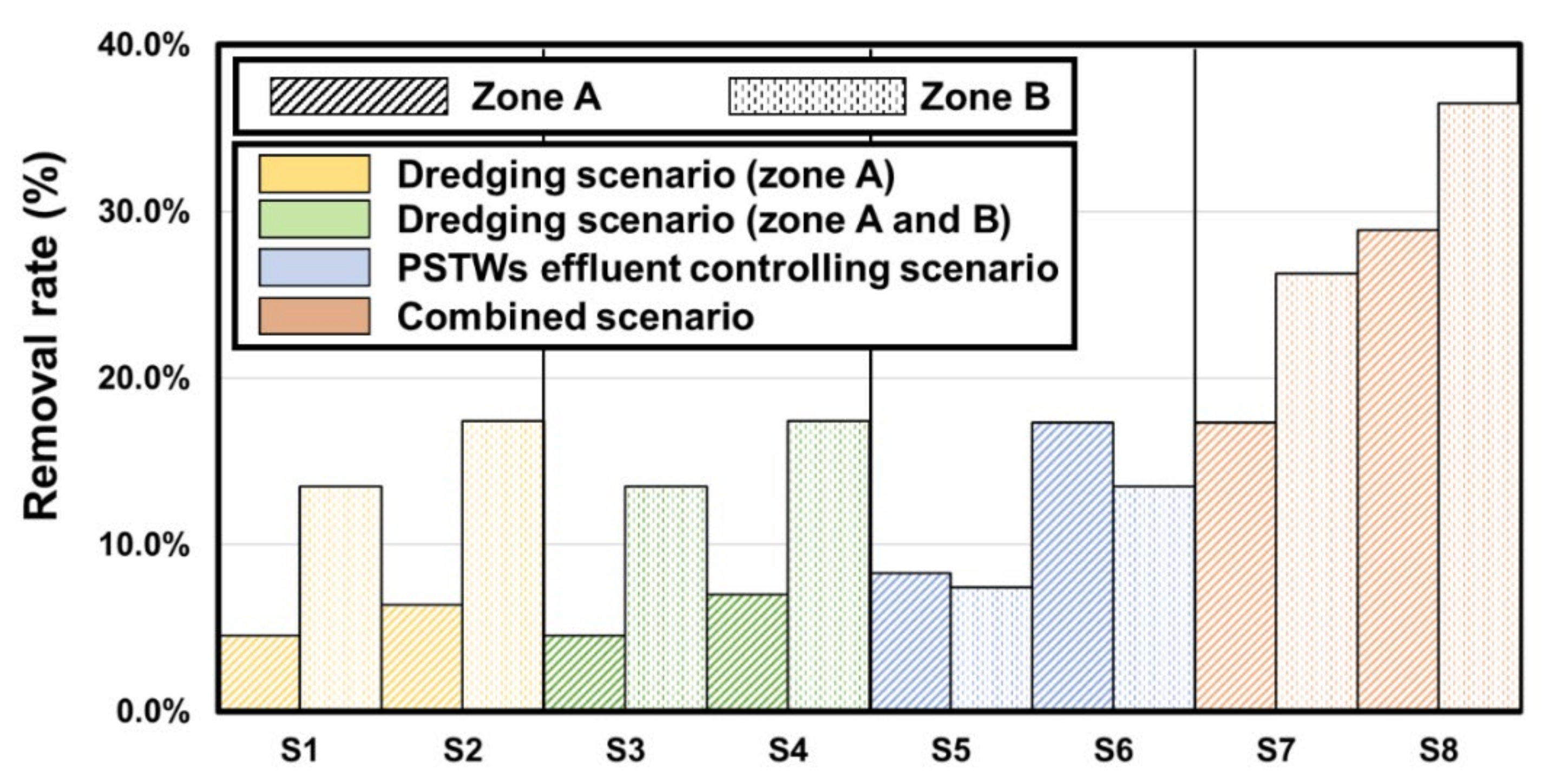
3.3. Total Phosphorus Reduction Efficiency Analysis Result

Figure 14 shows the total phosphorus reduction efficiency based on the water quality simulation results for each of the previous water quality improvement scenarios. In this study Figure 14 shows when only the soil improvement operation scenario was applied to Zone A (yellow column), when both the soil improvement scenarios were applied to Zone A and Zone B (green column) and the PSTWs’ effluents were treated (blue column), and when all scenarios were considered together (red column). In addition, Figure 15 shows the changes in water quality during a specific period for analyzing the total phosphorus reduction efficiency.

Regarding the T-P reduction efficiency of Zone A, the results are summarized as follows: S1, 4.6 %; S2, 6.4 %; S3, 4.6 %; S4, 7.0 %; S5, 8.3 %; S6, 17.3 %; S7, 17.3 %; and S8, 28.9 % mg/L. Regarding the T-P reduction efficiency of Zone B, the results are summarized as follows: S1, 13.5 %; S2, 17.4 %; S3, 13.5 %; S4, 17.4 %; S5, 7.4 %; S6, 13.5 %; S7, 26.3 % and S8, 36.5 % mg/L.

In both Zone A and Zone B, S1 and S3 show similar results, as do S2 and S4. This is because the level of soil contamination in Zone B is not relatively higher than that in Zone A (PO4-P benthic flux parameter in model (PO4D): 0.002 g/m²/d in Zone A, 0.001 g/m²/d in Zone B, and 0.0001 g/m²/d in Zone C). When comparing the results of Zones A and B, the effect of the water quality improvement by the dredging operation was greater in Zone B than in Zone A. This effect is significant because of some seawater circulation and the overall water quality improvement of the reservoir in Zone B (Figure 15a).

When the scenarios (S5, S6) to improve the quality of water discharged from the PSTWs were applied, there was a marked difference between Zones A and B. In the case of Zone A, the results of the discharged water improvement from the PSTW scenario were better than the improvement of the soil contamination scenario, indicating that the PSTWs significantly impacted the water quality in Zone A. In Figure 15b, it can also be seen that the water quality deteriorates rapidly because of the inflow of upstream water in Zone A. However, unlike the dredging scenario in Zone B, it can be seen that the effect of improving water quality is less than that of Zone A. Although improving water quality of the discharged water from the PSTWs reduces the external inflow load and decreases the system’s impact, its effect can be considered insignificant if the bottom soil of the estuarine reservoir is not improved. Therefore, these results reveal that reducing the estuarine reservoir’s internal load can increase its internal resilience by improving the bottom soil and have a significant effect on the overall water quality improvement.

4. Conclusions

This study evaluated the reduction efficiency of each water quality improvement scenario using the SWAT-EFDC linkage model for the Ganwol estuarine reservoir, which is experiencing water quality problems because of a continuous inflow of point and nonpoint source pollution from the upstream basin. In particular, because of the embankment located in the middle of the reservoir, it is necessary to analyze whether the effect of improving the water quality can be spread throughout the reservoir because of the location of a levee in the middle before applying the water quality management plan. Therefore, in this study, scenarios for reducing the external inflow load and internal load were applied, and the effects of the water quality improvement were analyzed by considering the levee’s influence.

If we look at the water quality changes of each location according to the effect of the water quality management plan, dredging improved the reservoir’s overall water quality by increasing its internal water quality. However, the PSTWs’ effluent management had a significant effect in improving the water quality in terms of reducing the inflow of pollutants, but the efficiency of Zone B was relatively lower than that of Zone A because of the levee’s influence. Therefore, in the current condition where the water quality in Zone A is worse than that in Zone B, it is appropriate to improve the water quality in the short term by improving the water quality discharged from the PSTWs. However, to improve the water quality of the entire reservoir in the long term, increasing the internal resilience by dredging can be considered to offset the levee’s impact.

This study evaluated water quality management scenarios using the SWAT-EFDC linkage model, which differs from other studies using the HSPF-EFDC linkage model; the difference is in the consideration of the nonpoint sources of pollution and farming mechanisms of agricultural land located around the reservoir. In addition, this study is meaningful because it comprehensively reviews the effects of embankments and water quality improvement scenarios and measures to improve resilience for improving water quality in reservoirs. In addition to evaluating the reservoir’s resilience, additional studies are needed to consider a management plan for improving water quality and increasing the resilience of the overall watershed and analyze its impact on the reservoir.

References

1. NOAA. Available online: https://oceanservice.noaa.gov/facts/estuary.html (accessed on 9 December 2020).
2. Gray, J.S. Marine biodiversity: Patterns, threats and conservation needs. Biodivers. Conserv. 1997, 6, 153–175. [Google Scholar] [CrossRef]
3. Schubel, J.; Kennedy, V.S. The Estuary as a Filter: An Introduction; Elsevier BV: Amsterdam, The Netherlands, 1984; pp. 1–11. [Google Scholar]
4. Jang, J.R.; Lee, S.H.; Cho, Y.; Choi, J.Y. A Calculation of Agricultural Water Demand According to the Farmland Developing Plan on the Saemangeum Tidal Land Reclamation Project. Korean Natl. Comm. Irrig. Drain. 2014, 21, 1–16. [Google Scholar]
5. Suh, S.-W.; Kim, J.-H.; Hwang, I.-T.; Lee, H.-K. Water quality simulation on an artificial estuarine lake Shiwhaho, Korea. J. Mar. Syst. 2004, 45, 143–158. [Google Scholar] [CrossRef]
6. Hwang, S. Dynamic Resilience Assessment for Water Quality Management of Estuarine Reservoir using SWAT-EFDC Model. Ph.D. Thesis, Seoul National University, Seoul, South Korea, 2020. [Google Scholar]
7. Conrad, S.R.; Santos, I.R.; White, S.; Sanders, C.J. Nutrient and Trace Metal Fluxes into Estuarine Sediments Linked to Historical and Expanding Agricultural Activity (Hearnes Lake, Australia). Chesap. Sci. 2019, 42, 944–957. [Google Scholar] [CrossRef]
8. Lee, Y.G.; Kang, J.-H.; Ki, S.J.; Cha, S.M.; Cho, K.H.; Lee, Y.S.; Park, Y.; Lee, S.W.; Kim, J.H. Factors dominating stratification cycle and seasonal water quality variation in a Korean estuarine reservoir. J. Environ. Monit. 2010, 12, 1072–1081. [Google Scholar] [CrossRef] [PubMed]
9. Song, Y.-H.; Choi, M.-S.; Ahn, Y.-W. Trace metals in Chun-su Bay sediments. J. Korean Soc. Oceanogr. Sea 2011, 16, 169–179. [Google Scholar] [CrossRef]
10. Lee, D.-K.; Kim, K.-H.; Lee, J.-S. Hypoxia and Characteristics of Nutrient Distribution at the Bottom Water of Cheonsu Bay Due to the Discharge of Eutrophicated Artificial Lake Water. J. Korean Soc. Mar. Environ. Saf. 2016, 22, 854–862. [Google Scholar] [CrossRef]
11. Park, H.S.; Lim, H.S.; Hong, J.S. Spatio and temporal patterns of benthic environment and macrobenthos community on subtidal soft- bottom in Chonsu Bay, Korea. J. Korean Fish. Soc. 2000, 33, 262–271. [Google Scholar]
12. Jha, D.K.; Devi, M.P.; Vidyalakshmi, R.; Brindha, B.; Vinithkumar, N.V.; Kirubagaran, R. Water quality assessment using water quality index and geographical information system methods in the coastal waters of Andaman Sea, India. Mar. Pollut. Bull. 2015, 100, 555–561. [Google Scholar] [CrossRef]
13. Nangia, V.; De Fraiture, C.; Turral, H. Water quality implications of raising crop water productivity. Agric. Water Manag. 2008, 95, 825–835. [Google Scholar] [CrossRef]
14. Liu, Z.; Hashim, N.B.; Kingery, W.L.; Huddleston, D.H.; Xia, M. Hydrodynamic Modeling of St. Louis Bay Estuary and Watershed Using EFDC and HSPF. J. Coast. Res. 2008, 10052, 107–116. [Google Scholar] [CrossRef]
15. Bicknell, B.R.; Imhoff, J.C.; Kittle, J.L.; Jobes, T.H.; Donigian, A.S. Hydrological Simulation Program-Fortran (HSPF). In User’s Manual for Release 12.2; Environmental Protection Agency: Washington, DC, USA, 2005. [Google Scholar]
16. Tetra Tech, Inc. The Environmental Fluid Dynamics Code User Manual Report; Environmental Protection Agency: Washington, DC, USA, 2007. [Google Scholar]
17. Zhang, Z.; Huang, J.; Zhou, M.; Huang, Y.; Lu, Y. A Coupled Modeling Approach for Water Management in a River-Reservoir System. Int. J. Environ. Res. Public Health 2019, 16, 2949. [Google Scholar] [CrossRef] [Green Version]
18. Loos, S.; Shin, C.M.; Sumihar, J.; Kim, K.; Cho, J.; Weerts, A.H. Ensemble data assimilation methods for improving river water quality forecasting accuracy. Water Res. 2020, 171, 115343. [Google Scholar] [CrossRef]
19. Kim, K.; Park, M.; Min, J.-H.; Ryu, I.; Kang, M.-R.; Park, L.J. Simulation of algal bloom dynamics in a river with the ensemble Kalman filter. J. Hydrol. 2014, 519, 2810–2821. [Google Scholar] [CrossRef]
20. Arnold, J.G.; Kiniry, J.R.; Srinivasan, R.; Williams, J.R.; Haney, E.B.; Neitsch, S.L. Soil and Water Assessment Tool Input/Output Documentation: Version 2012; Texas Water Resources Institute TR 439: College Station, TX, USA, 2012. [Google Scholar]
21. Zhu, K.-W.; Chen, Y.-C.; Zhang, S.; Yang, Z.-M.; Huang, L.; Li, L.; Lei, B.; Zhou, Z.-B.; Xiong, H.-L.; Li, X.-X.; et al. Output risk evolution analysis of agricultural non-point source pollution under different scenarios based on multi-model. Glob. Ecol. Conserv. 2020, 23, e01144. [Google Scholar] [CrossRef]
22. Volk, M.; Bosch, D.; Nangia, V.; Narasimhan, B. SWAT: Agricultural water and nonpoint source pollution management at a watershed scale. Agric. Water Manag. 2016, 175, 1–3. [Google Scholar] [CrossRef]
23. Zhang, P.; Liu, Y.; Pan, Y.; Yu, Z. Land use pattern optimization based on CLUE-S and SWAT models for agricultural non-point source pollution control. Math. Comput. Model. 2013, 58, 588–595. [Google Scholar] [CrossRef]
24. Shang, X.; Wang, X.; Zhang, D.; Chen, W.; Chen, X.; Kong, H. An improved SWAT-based computational framework for identifying critical source areas for agricultural pollution at the lake basin scale. Ecol. Model. 2012, 226, 1–10. [Google Scholar] [CrossRef]
25. Shen, Z.; Hong, Q.; Yu, H.; Liu, R. Parameter uncertainty analysis of the non-point source pollution in the Daning River watershed of the Three Gorges Reservoir Region, China. Sci. Total. Environ. 2008, 405, 195–205. [Google Scholar] [CrossRef]
26. Santhi, C.; Arnold, J.G.; Williams, J.R.; Hauck, L.M.; Dugas, W.A. Application of a Watershed Model to Evaluate Management Effects on Point and Nonpoint Source Pollution. Trans. ASAE 2001, 44, 1559–1570. [Google Scholar] [CrossRef]
27. Im, S.; Brannan, K.M.; Mostaghimi, S.; Kim, S.M. Comparison of HSPF and SWAT models performance for runoff and sediment yield prediction. J. Environ. Sci. Health Part A 2007, 42, 1561–1570. [Google Scholar] [CrossRef]
28. Hwang, S.; Jun, S.M.; Kim, K.; Kim, S.H.; Lee, H.; Kwak, J.; Kang, M.S. Development of a Framework for Evaluating Water Quality in Estuarine Reservoir Based on a Resilience Analysis Method. J. Korean Soc. Agric. Eng. 2020, 62, 105–119. [Google Scholar] [CrossRef]
29. Shin, S.; Her, Y.; Song, J.-H.; Kang, M.-S. Integrated sediment transport process modeling by coupling Soil and Water Assessment Tool and Environmental Fluid Dynamics Code. Environ. Model. Softw. 2019, 116, 26–39. [Google Scholar] [CrossRef]
30. Assaf, H.; Saadeh, M. Assessing water quality management options in the Upper Litani Basin, Lebanon, using an integrated GIS-based decision support system. Environ. Model. Softw. 2008, 23, 1327–1337. [Google Scholar] [CrossRef]
31. Kim, J.; Lee, S.; Shin, J.; Lim, J.; Na, Y.; Joo, S.; Shin, M.; Choi, J. Effect of Paddy BMPs on Water Quality and Policy Consideration in Saemangeum Watershed. J. Wetl. Res. 2018, 20, 304–313. [Google Scholar] [CrossRef]
32. Keipert, N.; Weaver, D.; Summers, R.; Clarke, M.; Neville, S. Guiding BMP adoption to improve water quality in various estuarine ecosystems in Western Australia. Water Sci. Technol. 2008, 57, 1749–1756. [Google Scholar] [CrossRef] [PubMed]
33. Fulton, M.H.; Moore, D.W.; Wirth, E.F.; Chandler, G.T.; Key, P.B.; Daugomah, J.W.; Strozier, E.D.; DeVane, J.; Clark, J.R.; Lewis, M.A.; et al. Assessment of risk reduction strategies for the management of agricultural nonpoint source pesticide runoff in estuarine ecosystems. Toxicol. Ind. Health 1999, 15, 201–214. [Google Scholar] [CrossRef]
34. Ioannidou, V.; Stefanakis, A.I. The Use of Constructed Wetlands to Mitigate Pollution from Agricultural Runoff. In Contaminants in Agriculture; Metzler, J.B., Ed.; Springer: Cham, Switzerland, 2020; pp. 233–246. [Google Scholar]
35. Xu, J.; Lo, S.L.; Gong, R.; Sun, X.X. Control of agricultural non-point source pollution in Fuxian lake with riparian wetlands. Desalination Water Treat. 2016, 57, 28570–28580. [Google Scholar] [CrossRef]
Figure 1. Diagram of the study watershed.
Applsci 11 03911 g001
Figure 2. Diagram of SWAT-EFDC linkage model for the estuarine reservoir system.
Applsci 11 03911 g002
Figure 3. Bottom elevation and levees of the estuarine reservoir in EFDC model.
Applsci 11 03911 g003
Figure 4. Locations of the dredging operation and PSTWs.
Applsci 11 03911 g004
Figure 5. (a) A comparison of the observed and simulated water levels and (b) changes to the water level elevation in the estuarine reservoir (2015–2017) [6].
Applsci 11 03911 g005
Figure 6. (a) Calibration and (b) validation result of the T-P concentration of the estuarine reservoir (Zone A).
Applsci 11 03911 g006
Figure 7. (a) Calibration and (b) validation result of the T-P concentration of the estuarine reservoir (Zone B).
Applsci 11 03911 g007aApplsci 11 03911 g007b
Figure 8. Simulated results of T-P concentration (Zone A, S0, S1–S4).
Applsci 11 03911 g008
Figure 9. Simulated results of T-P concentration (Zone A, S0, S5–S6).
Applsci 11 03911 g009
Figure 10. Simulated results of T-P concentration (Zone A, S0, S7–S8).
Applsci 11 03911 g010
Figure 11. Simulated results of T-P concentration (Zone B, S0, S1–S4).
Applsci 11 03911 g011
Figure 12. Simulated results of T-P concentration (Zone B, S0, S5–S6).
Applsci 11 03911 g012
Figure 13. Simulated results of T-P concentration (Zone B, S0, S7–S8).
Applsci 11 03911 g013
Figure 14. T-P removal rate results (Sn/S0, n = nth scenario).
Applsci 11 03911 g014
Figure 15. T-P concentration changes in the estuarine reservoir.
Applsci 11 03911 g015