Abstract
To achieve human-level object manipulation capability, a robot must be able to handle objects not only with prehensile manipulation, such as pick-and-place, but also with nonprehensile manipulation. To study nonprehensile manipulation, we studied robotic batting, a primitive form of nonprehensile manipulation. Batting is a challenging research area because it requires sophisticated and fast manipulation of moving objects and requires considerable improvement. In this paper, we designed a batting system for dynamic manipulation of a moving ball and proposed several algorithms to improve the task performance of batting. To improve the recognition accuracy of the ball, we proposed a circle-fitting method that complements color segmentation. This method enabled robust ball recognition against illumination. To accurately estimate the trajectory of the recognized ball, weighted least-squares regression considering the accuracy according to the distance of a stereo vision sensor was used for trajectory estimation, which enabled more accurate and faster trajectory estimation of the ball. Further, we analyzed the factors influencing the success rate of ball direction control and applied a constant posture control method to improve the success rate. Through the proposed methods, the ball direction control performance is improved.
1. Introduction
To date, a variety of robots have been used in automated production lines for object manipulation tasks in factories, and these robotic technologies have contributed significantly to the development of modern industry. Recently, with the fourth industrial revolution, robots have been introduced to provide various services not only in factories but also in human living environments. Robots used in factories perform simple repetitive operations such as pick-and-place using specially designed grippers; however, in an environment such as cafes and restaurants, human-level object manipulation ability is required. Therefore, to provide a wider range of services in a human living environment, robots must have a higher level of object manipulation similar to that of humans.
In addition to manipulating objects using grasping, humans can manipulate objects freely by appropriately utilizing nonprehensile manipulations [1] without grasping, such as throwing, batting, rolling, pushing, and sliding. Most robots are still limited to prehensile manipulation using grasping. A robot that performs nonprehensile manipulation is rare owing to the difficulty of control using nonprehensile manipulations. When nonprehensile manipulation is performed, the object moves during manipulation. Since the moving object is not fixed to the robot, it is necessary to plan and control the future behavior of the moving object based on the state of the robot and the moving object. Despite these difficulties, nonprehensile manipulation has advantages such as increased object manipulation methods, expansion of the robot workspace, and increased manipulation dexterity [2]. To improve the ability of robots to manipulate objects, the robots must have nonprehensile manipulation capabilities with these advantages.
Fabio et al. conducted a survey on nonprehensile manipulation of robots to address the trends and open issues of nonprehensile manipulation studies [3]. According to [3], the nonprehensile manipulation task is complex and difficult. Because of the complexity and difficulty of the task, most studies divide the nonprehensile manipulation task into simpler subtasks called nonprehensile manipulation primitives. The representative nonprehensile manipulation primitives include throwing [4], catching [5], batting [6], pushing [7], sliding [8], and rolling [9]. Each of these nonprehensile manipulation primitives is selectively operated by a high-level supervisor depending on the task [10]. Among the nonprehensile manipulation primitives, batting is challenging because it requires precise and fast manipulation of the moving objects, and studies on this topic are lacking. In sporting events such as table tennis, tennis, and baseball, players have a batting ability to send the moving objects (balls) to the desired position with sophisticated and quick manipulation, while the batting performance of robots is insufficient. Therefore, this study aims to contribute to the improvement of the dexterity of robots by conducting research on batting, which requires more precise and quicker nonprehensile manipulation of moving objects than do the above-mentioned primitives.
For a robot to perform a batting task, at least four methods are required. First, image processing is required to recognize a moving ball. Second, estimation of the future trajectory of the ball is required. Third, the motion of the robot arm must be controlled to affect the ball direction. Lastly, calibration is required to convert the coordinates between the robot arm’s coordinate system and the vision sensor’s coordinate system. This implies that the performance of each method affects the performance of the batting primitive; studies that can improve the performance of each method are discussed.
Chen et al. [11] developed a vision module for humanoid robotic table tennis. The vision module contains two stereo vision sensors with a 200 fps and an algorithm for predicting the rebound trajectory of a table tennis ball. Nakabo et al. [12] developed a high-speed vision system capable of image acquisition and image processing at 1 kHz for moving ball recognition. A parallel computation architecture was used to reduce image transfer and processing time, and an active vision system with moving cameras was developed to track the moving objects. Tesheng et al. [13] used an aerodynamic model of a ball to account for the trajectory of the ball before and after collision to improve the performance of ball direction control. Serra et al. conducted the study of hitting a table tennis ball to the desired position [14]. To accurately control the arrival position of the ball after hitting, a more accurate aerodynamic model that that in [13] was applied for the trajectory estimation of the ball. Although the algorithms were tested via simulations, the implementation of the algorithms on an actual hardware system was left to be covered under future work. For accurate ball direction control, a batting algorithm considering impact dynamics was proposed [15,16]; however, the problem of extending the 2D algorithm to the 3D algorithm remains due to the computation time required for impact dynamics in 3D.
Schüthe et al. [17] introduced the optimal control with state and soft constraints for a simulated ball batting task. By utilizing the soft constraints, a motion utilizing the redundant degree of freedom (DOF) is automatically generated, but there is a limitation in that a motion exceeding the range of motion of the joint is generated. Pekarovskiy et al. [18] proposed a motion generation method that can adapt to rapidly changing target points in consideration of the feasibility and computation time of the motion trajectory. This method was applied to 2D planar volleyball batting. Kober et al. [19] proposed a method to generate the trajectory of the robot arm through learning. If the system is changed, the process of collecting and processing data is required again, and the ball direction control is not considered. Mori et al. [20] developed a fast and lightweight robotic arm for badminton. The use of pneumatic actuators made the robotic arm lighter, enabling high-speed batting. The position of the shuttlecock was measured using a high-speed motion capture system of 240 Hz, but there was a limitation in that control of the direction of the ball was generated by a pre-learned feedforward motion. In the realization of a three-dimensional ball direction control system, the amount of computation in object recognition and trajectory estimation and the realizable three-dimensional motion generation are important.
Senoo et al. [21] developed a high-speed robot batting algorithm using a high-speed active vision system developed by Nakabo et al. [12]. The algorithm was extended to control the direction of the baseball in three-dimensional space [22]. For fast batting and ball direction control, the authors proposed a hybrid trajectory generator comprising a part that generates a high-speed batting motion and a part that modifies the motion through visual feedback. A high-speed image processing system (1 kHz) specially developed for object recognition was used, and a simple least square method was applied to estimate the object trajectory because the sampling rate was fast. Without this specially designed sensor system, it is difficult for other researchers to implement a batting system using this algorithm.
In this study, we propose a batting framework capable of controlling the three dimensional direction of a moving ball by using an off-the-shelf vision sensor with a relatively low fps (50 Hz). The proposed batting framework includes object recognition, object trajectory estimation, robot arm motion control, and calibration. In a condition where the image sampling rate is low, since the importance of one data point is relatively large, the performance of algorithms for object recognition, trajectory estimation, and motion control becomes more important. Therefore, we propose ways to improve the performance of each algorithm at a low sampling rate. Since the proposed methods were developed based on an off-the-shelf vision sensor, other researchers can easily implement these algorithms.
The specific contributions of this study are as follows. First, in terms of ball recognition, this study proposes an image processing method for improving ball recognition accuracy in a more general environment. Previous studies covered noise filtering after applying a difference image or color segmentation. In the real world, however, various lights affect the ball recognition accuracy. Further, we applied the method using the geometrical properties of the ball to improve the recognition accuracy under these lighting conditions. Second, by applying weighted squares regression considering the positional accuracy according to the distance of the stereo vision sensor, we improve the trajectory estimation accuracy of the target object even with a low sampling rate. Third, we analyze the factors that affect the performance of ball-direction control and propose additional constant posture control methods to reduce the influence of those factors. Finally, in actual implementation, calibration between the camera and the robot coordinate system is essential. A simple but accurate calibration method is introduced.
2. Robot Batting System
We built a robot betting system as shown in Figure 1. The hardware of the batting system consists of a stereo vision sensor for recognizing the red ball and obtaining positional information in three-dimensional space, and a six DOF robotic arm for batting the ball to the target position (Net in Figure 1). The stereo vision sensor (Bumblebee2, Point Gray Research Inc.) provides 640 × 480 pixels color images at up to 48 frames per second (fps). The Triclops library included in Bumblebee2 (Point Gray Research Inc.) provides 3D position coordinates. Bumblebee is shipped with precision calibration at the production stage, and because the two cameras are structurally fixed, there is no need to perform additional calibration between the two cameras. A slightly modified version of the arm of a humanoid robot, Hubo [23], designed by the HUBO LAB of the Korea Advanced Institute of Science and Technology, was used for batting. Link lengths were changed to extend the workspace, and the robotic hand end device was replaced with a 0.09 m diameter round aluminum plate to perform the batting task.
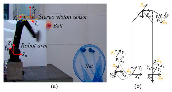
Figure 1.
(a) Robotic batting system. The hardware of the batting system consists of a stereo vision sensor and a six degree of freedom robotic arm. (b) Robot arm configuration. The base coordinate system of the robot arm is the first coordinate system.
3. Method
We applied a color segmentation method [24] to recognize the red ball. To improve the recognition accuracy of the ball under the conditions of illumination, a circle fitting method [25] using the geometrical characteristics of the ball is employed.
3.1. Ball Recognition
3.1.1. Color Segmentation
The color separation method is used to find pixels with specific color values in the image. Since we used a red ball in the batting experiment, only red is segmented in the image by comparing the red component () and the threshold value () of the pixel as shown in Equation (1).
For improved visualization, the color image is converted to a binary image comprising pixels () with only two values. The pixels corresponding to the threshold value or more are represented by “1” (white), and the other pixels are represented to “0” (black); thus, the red ball becomes white. However, since the RGB value changes according to the change in illuminance, not only the ball but also noise are binarized. To remove this noise, the morphology method [26] is applied. This method is effective for removing the salt-and-pepper noise or impulse noise between objects and the background. Figure 2 shows the results of finding the location of the ball on the desk in the lab when color segmentation and morphology methods are applied. The left side of the figure is a color image, the right side is a binary image, and only the red ball appears white in the binary image.
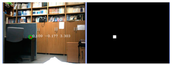
Figure 2.
Color image (left) and binary image (right). Green circle of color image represents the position of the red ball.
3.1.2. Circle Fitting
Figure 3a shows the batting experiment environment captured using a stereo vision camera. Because the ceiling light creates a shadow on the lower part of the ball, the RGB value of the lower part of the ball changes. Figure 3b shows a binarized image with color segmentation applied to the image in Figure 3a. In the binary image of Figure 3b, the shape of the ball appears as a semicircle rather than a circle because the lower part of the color change is not properly color segmented. Incorrect color segmentation causes errors in the center position measurement of the ball. For example, if only the upper part of the ball is color-segmented, the position error in the vertical direction increases. Threshold adjustment is limited because the difference between the color value of the lower part of the ball and the color value of the upper part is large.
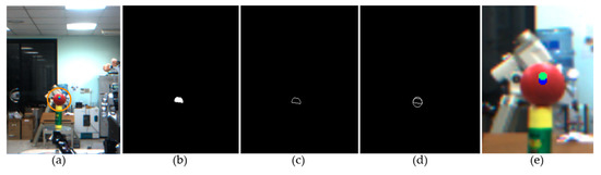
Figure 3.
Circle fitting process. (a) Batting experiment environment captured using a stereo vision camera, (b) A binary image with color segmentation, (c) The edge image of the semicircle, (d) An image with circle fitting applied to the edge of a semicircle, (e) Center position before (green) and after (blue) circle fitting.
To overcome the limitations of color segmentation, we additionally applied a circle fitting method that uses the geometric characteristics of a circular ball. Figure 3c shows only the edge of the semicircle shown in Figure 3b. By applying a circle fitting to the edge of the semicircle, we can estimate the original circle ball shape, as shown in Figure 3d. Figure 3e shows the center position of the ball before applying the circle fitting (lime green point) and the center position of the ball after application (blue point). The positions of the lime green and blue points are (X, Y, Z) = (−0.0416, 1.3299, −0.0888) and (X, Y, Z) = (−0.0413, 1.3207, −0.0955), respectively. The true position of the ball is (X, Y, Z) = (−0.0414, 1.3187, −0.0985). Prior to the circle fitting method, the error in the z direction was 0.0097 m, which is approximately 20% of the diameter of the ball at 0.05 m. After the circle fitting method was applied, the center position of the ball moved by about 0.007 m further down the Z-axis, and the position error in the Z direction was reduced from 0.0097 m to 0.0030 m.
3.1.3. Calibration
Since the position of the ball measured in the vision coordinate system needs to be converted to the robot coordinate system, a coordinate transformation between the two coordinate systems is required. For coordinate transformation between two coordinates, we attached the red marker shown in Figure 4 to the end-effector of the robot arm and measured its position in the vision coordinate system and the robot coordinate system. Coordinate transformation between two coordinates is possible using a homogeneous transformation matrix representing the relationship between the camera coordinate system and the robot base coordinate system, as shown in the following equation:
where .
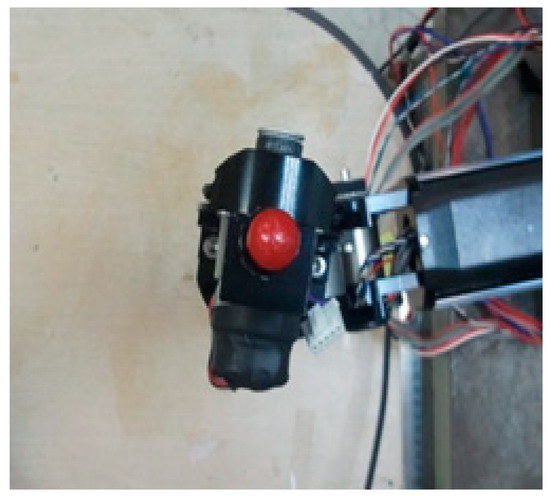
Figure 4.
Red marker attached to the end-effector of the robotic arm to calculate the homogeneous matrix.
Subscripts B and C represent the robot arm base coordinate and camera coordinate systems, and represent the positions of the markers (Figure 4) measured in the robot and vision coordinate systems, respectively, denotes the homogeneous transformation matrix, and and represent the rotation matrix and the distance vector between the robot coordinate system and the camera coordinate system, respectively. The homogeneous transformation matrix can be calculated by the least square method as
E and V consist of the position vectors of the markers measured in the robot coordinate system and the vision coordinate system, respectively, and N is the number of measured position vectors. From the base coordinate system of the robot, the position data set … is calculated by forward kinematics. The position data set … is measured using the stereo vision sensor.
The accuracy of coordinate transformation is improved by calculating a homogeneous matrix from data measured at various locations as shown in Figure 5. From the measured data, the homogeneous transformation matrix is calculated as
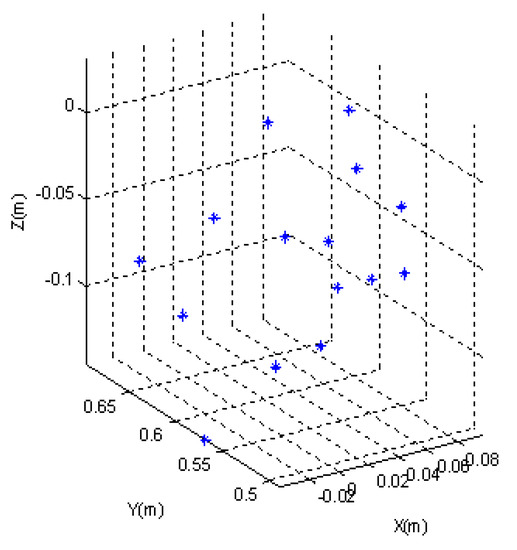
Figure 5.
Red marker positions measured from the vision sensor. The positions of the markers measured at various positions are used to accurately calculate a homogeneous matrix.
From and of the homogeneous transformation matrix, the camera coordinate system is at a distance of 0.1935 m in the X-axis direction, 0.8037 m in the Y-axis direction, and 0.3792 m in the Z-axis direction from the robot coordinate system. In the robot coordinate system, the camera coordinate system is rotated by 0.3188° for the X axis, 0.6539° for the Y axis, and 178.9466° for the Z axis. To evaluate the accuracy of the calculated homogeneous transformation matrix, the positions of the markers obtained from the homogeneous transformation of the marker positions measured in the vision are compared with the positions of the markers measured in the robot coordinate system as shown in Figure 6. The error is expressed as a norm value for the X, Y, and Z axes. The mean error is 0.0024 m and the standard deviation is 0.0012 m. Considering that the error is less than 0.005 m and the diameter of marker is 0.01 m, the calculated homogeneous matrix is sufficiently accurate.
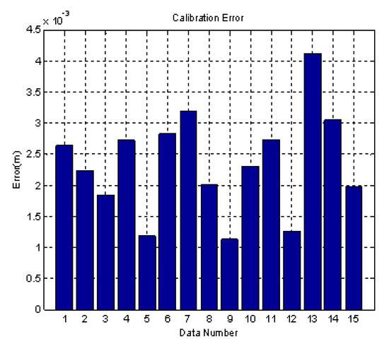
Figure 6.
Histogram showing the calibration error for 15 marker positions.
3.2. Ball Trajectory Estimation
Considering the limitations of the joint speed, the robot arm should be able to move in advance by estimating the trajectory of the ball. To estimate the trajectory of the ball, we used weighted least-squares regression [27]. Each time a new ball position and time is acquired by the vision sensor, the trajectory of the ball is updated using weighted least-squares regression.
3.2.1. Least Square Regression
The x and y planes of the robot coordinate system are horizontal planes and the z direction is perpendicular to the x-y plane. A linear function was used to estimate the horizontal trajectory of the ball, and a quadratic function was used to estimate the vertical trajectory. Because the ball moves in a parabolic trajectory, the z-axis trajectory of the ball is fitted as a quadratic function, unlike other axes. The trajectory function for each of the x, y, and z axes of the ball is given by
Whenever three-dimensional position data are newly measured in the stereo vision sensor, the coefficient of the trajectory function (5) is newly calculated through least square regression [28]. The position data sampling interval of the ball is 20 ms, which is the image acquisition period of the stereo vision sensor. Since the flight time of the ball is 0.5 s on average, approximately 15 to 20 ball position data points are measured. Figure 7 represents the estimated trajectory of the ball according to the number of data points using least squares regression. As the number of data points increases, it can be seen that the estimated trajectory converges to one trajectory.
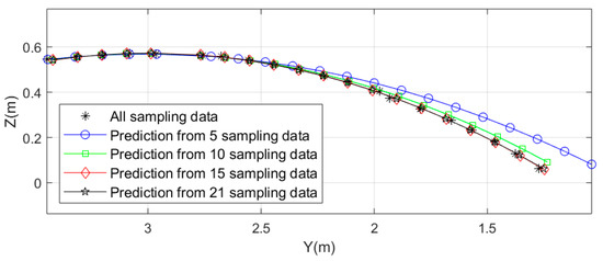
Figure 7.
Estimated ball trajectory according to the number of sampled data points. As the number of sampled data points increases, the trajectory estimation becomes more accurate.
3.2.2. Weighted Least Square Regression
Least square regression was applied to the ball trajectory estimation regression described in Section 3.2.1, based on the assumption that the data measured by the stereo vision sensor are accurate. However, the accuracy of the position data measured from the stereo vision sensor is inversely proportional to the distance between the stereo vision sensor and the object. This is because the closer the distance, the greater is the number of pixels representing the object. Figure 8 shows a graph of position accuracy versus distance between Bumblebee2 and the object. Therefore, it is more appropriate to apply the weighted least-squares regression than the least-squares regression considering the accuracy of the measured value according to the distance.
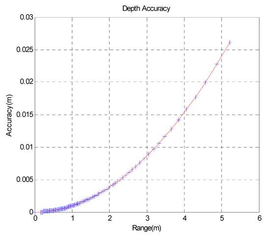
Figure 8.
Depth error vs. distance. Depth accuracy of stereo vision sensor according to distance.
Least squares regression minimizes the sum of the squares of the residuals, and the weighted least-squares regression minimizes the sums (Q) of the squares of the residuals () multiplied by the weight (); it is given by
The weights are calculated as a geometric sequence based on the last weight. In several tests, 0.8 was used as of the weighted least square. Figure 9 is a graph showing the RMS errors for the X, Y, and Z components obtained by applying the weighted least square and least square regressions. Although there is almost no difference in the RMS error for X and Y with and without the weighted least square, the RMS error decreases rapidly with weighted least square for the Z axis. This result is expected because the change in the trajectory of the ball on the z axis is larger than that on the x and y axes.
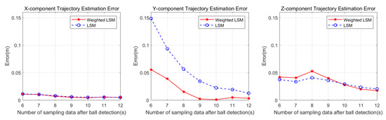
Figure 9.
RMS error vs. sampling data number about the x axis. RMS error of the estimated ball trajectory with and without weighted least squares method. RMS error for each axis is displayed in the order of X axis, Y axis, and Z axis from the left.
3.3. Motion Control of the Robot Arm
The trajectory of the robot arm consists of two stages: before and after batting. The speed of the end-effector of the robot arm increases before batting, and after batting, a trajectory is generated that slows down the increased speed of the end-effector. The robotic arm used in the experiment has six joints, and, therefore, we need to generate the trajectories of the six joints. For convenience, the joint trajectory generation method is described by the notation of one joint, and the same method is applied to the remaining joints. The trajectory generation method before batting is described first, followed by the trajectory generation method after batting.
The cubic spline interpolation function for generating the motion trajectory of a joint is:
where is the coefficient of the trajectory function and t is the time. Since coefficients in Equation (7) are four, four constraints are needed to obtain each coefficient. The constraints of the trajectory function before hitting the ball are as follow:
3.3.1. Trajectory Interpolation
The trajectory constraints of Equation (8) represent the initial joint position , joint position to hit the ball, initial joint velocity , and velocity to hit the ball. and represent the initial position of the joint and the joint position at the moment of hitting the ball, represents the time of the moment of hitting the ball, and represents the angular velocity vector at the moment of hitting the ball. Four simultaneous equations are constructed according to four constraints, and each coefficient can be obtained by calculating the simultaneous equations.
After hitting the ball, a joint trajectory has to be generated to reduce the speed of the robot arm. By calculating the simultaneous equations with the following four constraints, a joint trajectory is generated to decrease the velocity of robot arm.
The initial joint position is the angle to hit the ball, the final joint position is the angle in the configuration where the robot arm stops, the initial velocity is at the time of the hit, the final velocity is 0, and is the time to stop.
3.3.2. Robot Batting Trajectory
The angular and velocity trajectories of joints 1 and 3 for when the batting task is performed as generated by the cubic spline function and constraints are shown in Figure 10. Through cubic spline interpolation, the trajectories of the joints were smoothly interpolated from the initial position before batting to the stop position after batting. The batting time is 0.274 s and the time it takes for the robot arm to stop completely after it starts moving is 0.914 s. The maximum angular velocity is given only to joints 1 and 3 because the maximum angular velocity of the other joints is limited and has little effect on the speed of the end-effector. After hitting, the robot arm stops smoothly by imposing a constraint on the angular velocity of joints 1 and 3 as 0. The velocity of the end-effector is calculated as
where ,
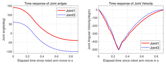
Figure 10.
The angular and velocity trajectories of joints 1 and 3. When the robot arm hits the ball, the joint angular velocity of joint 1 and joint 3 was constrained to −500°/s, and the rest of the joints to zero.
is the Jacobian matrix of the robot arm, and is a vector consisting of the angular velocities of the joints of the robot arm. The calculated velocity of the end-effector is 6.2 m/s.
3.3.3. Ball Direction Control
The ultimate goal of the batting task is to move the object to the desired target position in a single collision. The orientation of the end-effector of the robot must be controlled to move the ball to the desired target position. That is, the direction of the ball after the collision can be controlled by controlling the normal vector perpendicular to the circular plate of the end-effector. The normal vector can be calculated from the coefficient of restitution between the ball and the end-effector, the velocity of the ball and the end-effector before and after the collision, and some assumptions. Figure 11 shows the velocity vector of the ball before the batting (), the velocity vector of the ball after the batting (), and the velocity vector of the end-effector of the robot () and the normal vector () perpendicular to the plane of the end-effector.
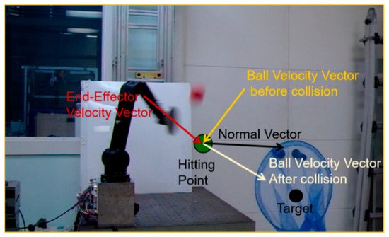
Figure 11.
Vector arrangements representing end-effector velocity (), ball velocity before collision (), ball velocity after collision (), and normal vector ().
The vector shown in Figure 11 can be expressed as shown in Figure 12 under the assumption that there is no change in the velocity of the end-effector before and after the collision, and that there is only energy loss caused by the deformation of the ball in the collision.
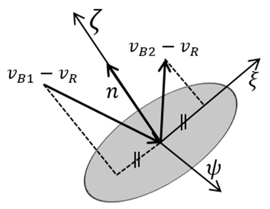
Figure 12.
Vector analysis before and after collision.
From Figure 12, the relationship between the velocity vectors and the normal vector can be defined by the collision coefficient equation
The collision coefficient (e) is the speed ratio before and after the collision of the ball, and the material of the ball and the end device has a major influence on the collision coefficient. Considering the inherent properties between the ball and the end-effector, we obtained the collision coefficient through collision experiments. The coefficient was obtained by dropping the ball perpendicular to the end-effector to measure the speed before and after the impact. The average collision coefficient obtained from 20 experiments is 0.6506 and the standard deviation is 0.0448. Based on the assumptions above, the velocity of the horizontal component before and after the collision of the ball is preserved and can be expressed as
The above equation can be rearranged as
Note that the normal vector is in the same direction as that of the difference in the velocity vector before and after the collision of the ball. Therefore, the information of and is needed to calculate . The is calculated by differentiating Equation (5), and the direction of is calculated from the estimated trajectory of the ball and the target position. Therefore, to calculate the normal vector, it is necessary to calculate the magnitude of the .
The direction of the velocity vector after the collision is derived from the vector geometry. The velocity vector after the collision in Figure 12 can be set to one side of the triangle as shown in Figure 13. is the direction vector of , and represents the horizontal relative velocity vector that is preserved before and after the collision of the ball. The Pythagorean theorem applies to the two triangles and and is represented by the following two equations:
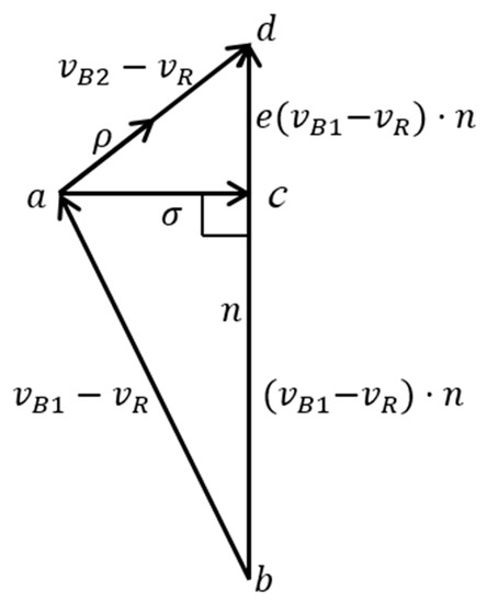
Figure 13.
Vector analysis.
The difference between the two equations is
The cosine law is applied to as
From Equations (16) and (17), we can calculate the relative velocity of the ball after the collision as
From Equations (13) and (18), the normal vector perpendicular to the circular plate of the terminal end-effector can be expressed as
From the calculated normal vector, the orientation of the ball after the collision is adjusted by adjusting the orientation of the robot end-effector.
4. Experiment
4.1. Batting Experiment
The batting task was performed based on the algorithms proposed in the previous sections. Snapshots of the robot arm hitting the oncoming ball to the target are shown in Figure 14. The target position for the ball is a blue net that is 0.57 m in the x-axis, −0.48 m in the y-axis, and −0.09 m in the z-axis from the robot base coordinate. We performed the experiment in the same way by changing the position of the target to 0.36 m for the x-axis and 1.06 m for the y-axis to −0.02 m for the z-axis. We conducted 30 batting experiments each, the success rate converged to approximately 40%.
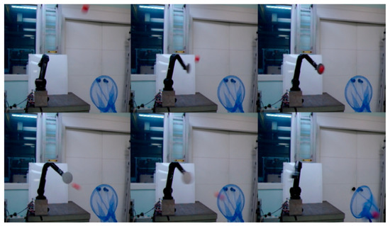
Figure 14.
Successive snapshots of batting task (sequence is horizontal to vertical).
We conducted two additional experiments to analyze the factors that influence the success rate. Since the trajectory prediction function of the ball is a function of position versus time (Equation (5)), the arrival position estimation error of the ball and arrival time estimation error of the ball are analyzed. If there is a large error in the estimated ball position or time, this error will affect the success rate of the batting task.
4.2. Experiment to Analyze the Predicted Ball Position Accuracy
We stopped the robotic arm at the predicted ball position without swinging to analyze the estimated ball position accuracy. We will call this experiment a bunt experiment, similar the action of the same name in a baseball game. The effect of the time error was separated by placing the end-effector of the robot arm at the position where the ball arrived. Thirty experiments were carried out, and the robotic arm was able to touch all the thrown balls (success rate is 100%). This experiment shows that the estimated ball position is accurate for ball batting. Figure 15 shows the positions of the batted balls in 30 experiments.
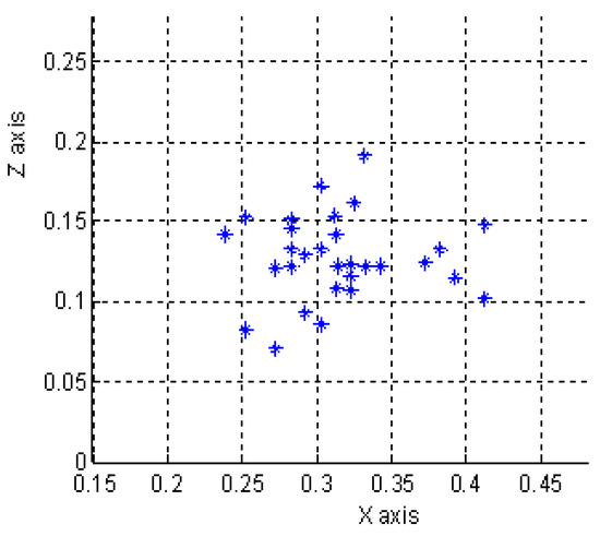
Figure 15.
Shot group of the batted ball. In this bunt experiment, the robotic arm hit the ball with a 100% success rate.
4.3. Experiment to Analyze the Accuracy of the Predicted Ball Arrival Times
Data acquired from the stereo vision sensor includes time information together with image data. The time information is measured at the moment the shutter of the camera is closed, and this time information is called a time stamp. The timer cycle of the camera is 8 kHz, and a time stamp is calculated based on this cycle.
A red marker (Figure 4) was attached to the end-effector of the robot arm, and the position and time of the marker was measured with a vision sensor. To measure the time difference between each image, the robot arm drew a circle at a constant velocity of 17 degree/s with respect to the Y-Z plane. While the robot arm moved in a constant velocity circular motion, time information was measured along with the position of the marker. Figure 16 shows the marker positions of the end-effector when the robot arm moved at constant speed. A histogram comparing the time difference between two theoretical positions caused by constant circular motion and the time difference measured using a vision sensor is shown in Figure 17. The mean time difference error was −0.00057 s and the standard deviation was 0.0048 s. If the error pattern is biased, the time difference error can be compensated; however, in the case of such a random error, it is difficult to compensate for the time difference error. Therefore, the following section describes the proposed method to compensate for the time error.
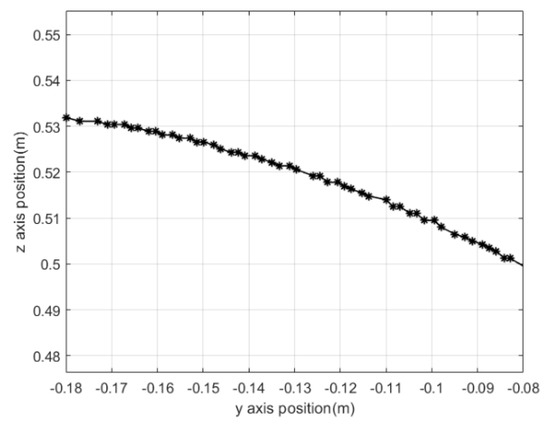
Figure 16.
Marker position from vision sensor.
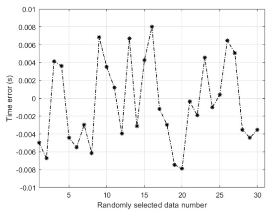
Figure 17.
Time error for randomly selected data. Time error shows a random error pattern.
4.4. Constant Posture Control Method
Time errors change the timing of the hitting. Accordingly, the success rate of ball direction control is decreased. To compensate for this time error, we propose a method of maintaining the posture of the end-effector for a predetermined time before and after the ball hitting, and this method is called the constant posture control (CPC) method. By maintaining the posture of the end-effector for a predetermined time before and after the hitting timing, the posture change of the end device due to time error is prevented. We set the time that the posture of the end-effector should be maintained to a total of 0.3 s with 0.015 s before and after the hit.
We conducted a ball direction control experiment to verify the effectiveness of the CPC method. Figure 18 shows the posture change of the end-effector with and without the CPC method while the robot arm swings. Postures are expressed in Euler angles. The solid line is a change in posture considering the CPC method, and the dotted line is a change in posture without considering the CPC method. Since the robot arm strikes the ball while rotating about the Z axis (refer to the axis in Figure 1), the Euler angle change about the Z axis is very large. For a clear comparison, the experimental results are described based on the Z axis Euler angle. The interval in which the posture should be kept is between 0.222 s and 0.252 s. The red solid Z-axis Euler angle was in the range of −76.79° to −77.63°. This is a negligible error compared to the Z axis Euler angle of −77.16° to be maintained. On the other hand, the blue dotted line without considering the CPC method shows that the Z-axis Euler angle was changed from −73.24° to −82.81°. Finally, after 15 experiments, the success rate was 53.0% when considering the CPC method, and the success rate was increased by 13% when the CPC method was not considered. The experimental video is shown in [29].
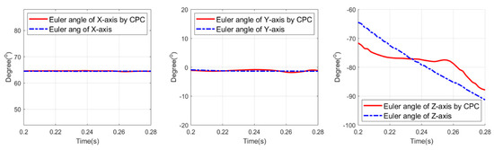
Figure 18.
Posture change of end-effector with and without constant posture control (CPC) method.
5. Discussion
In this paper, we designed a ball batting system to perform batting tasks and proposed algorithms to improve the success rate of ball direction control under low sampling rate conditions. In a condition where the image sampling rate is low, since the importance of one data point is relatively large, the performance of algorithms such as object recognition and trajectory estimation becomes more important. In terms of object recognition, we applied a circular fitting method that is robust to the influence of illuminance and improved the 3D position accuracy of the ball by about 60% compared to the conventional image processing method with color segmentation and noise filtering applied. In terms of trajectory estimation, while the conventional method uses complex models, we proposed a weighted least square trajectory estimation method based on a simple model. As shown in Figure 9, it is possible to accurately estimate the trajectory with a small number of data points by considering the weight according to the distance. In terms of motion control of the robot arm, through analysis of the factors affecting the success rate of ball direction control, a time error, which is a random error, was found as shown in Figure 17, and a constant posture control method was proposed to overcome this. Through this method, the ball direction control success rate was improved by about 13%.
The methods proposed in this study can be applied to other research fields. The ball recognition method using geometric features can be used to improve recognition accuracy of other objects. Since the ball trajectory estimation method using the weighted least squares method can overcome the problem of computation time in the conventional complex model-based trajectory estimation method, this method can be applied not only at low-speed sampling times but also at high-speed sampling times. In addition to the trajectory estimation field, the algorithm considering the accuracy of the stereo vision sensor according to the distance can be easily applied to other stereo vision applications, and thus can be used as an effective performance improvement method.
Although the current ball direction control success rate is similar to that of research using high-speed vision sensors, there is a possibility that the success rate will be further improved if the algorithms proposed in this study are applied to a batting system equipped with a high-speed vision sensor. In addition, if the currently used ball model is improved, the accuracy of ball trajectory estimation is expected to be further improved. We plan to study the trajectory estimation method that combines the improved ball model and the weighted least squares method.
6. Conclusions
We conducted research on batting, one of the primitives of nonprehensile manipulation. We designed a ball batting system to perform batting tasks and proposed algorithms to improve the success rate of ball direction control under low sampling rate conditions. The recognition accuracy of the ball was improved by applying the color segmentation method and the circle fitting method to the recognition of the ball. In consideration of the measurement accuracy according to the distance of the stereo vision sensor, the estimated trajectory of the ball was predicted more accurately and in a faster manner by applying weighted least square regression to the ball trajectory estimation. A method of controlling the posture of the end-effector of the robot arm to control the direction of the ball was presented, and a smooth robot arm trajectory was generated while satisfying the constraints and adapting to the target trajectory. Furthermore, we analyzed the factors affecting the ball direction control and proposed a method of maintaining the end position of the robot arm to compensate for the time uncertainty. Through this, the posture of the end-effector was kept constant before and after hitting, and the success rate of the ball direction control was increased by about 13%.
Author Contributions
Conceptualization, H.-M.J.; Formal analysis, H.-M.J. and J.-H.O.; Funding acquisition, J.-H.O.; Investigation, H.-M.J.; Methodology, H.-M.J. and J.-H.O.; Resources, J.L.; Software, H.-M.J. and J.L.; Supervision, J.-H.O.; Validation, H.-M.J.; Visualization, H.-M.J.; Writing–original draft, H.-M.J. and J.-H.O.; Writing–review & editing, H.-M.J. and J.L. All authors have read and agreed to the published version of the manuscript.
Funding
This work was supported by the National Research Foundation of Korea (NRF) grant funded by the Korea government (Ministry of Science and ICT) (No. NRF-2020R1G1A1101767 and No. NRF-2020R1C1C1008520).
Conflicts of Interest
The authors declare no conflict of interest.
References
- Lynch, K.M.; Mason, M.T. Dynamic nonprehensile manipulation: Controllability, planning, and experiments. Int. J. Robot. Res. 1999, 18, 64–92. [Google Scholar] [CrossRef]
- Ruggiero, F.; Petit, A.; Serra, D.; Satici, A.; Cacace, J.; Donaire, A.; Ficuciello, F.; Buonocore, L.; Fontanelli, G.; Lippiello, V.; et al. Nonprehensile manipulation of deformable objects: Achievements and perspectives from the robotic dynamic manipulation project. IEEE Robot. Autom. Mag. 2018, 25, 83–92. [Google Scholar] [CrossRef]
- Ruggiero, F.; Lippiello, V.; Siciliano, B. Nonprehensile dynamic manipulation: A survey. IEEE Robot. Autom. Lett. 2018, 3, 1711–1718. [Google Scholar] [CrossRef]
- Satici, A.C.; Ruggiero, F.; Lippiello, V.; Siciliano, B. A Coordinate-Free Framework for Robotic Pizza Tossing and Catching. In Proceedings of the 2016 IEEE International Conference on Robotics and Automation (ICRA), Stockholm, Sweden, 16–21 May 2016; pp. 3932–3939. [Google Scholar]
- Bätz, G.; Yaqub, A.; Wu, H.; Kühnlenz, K.; Wollherr, D.; Buss, M. Dynamic Manipulation: Nonprehensile Ball Catching. In Proceedings of the 18th Mediterranean Conference on Control and Automation, MED’10, Marrakech, Morocco, 23–25 June 2010; pp. 365–370. [Google Scholar]
- Serra, D.; Satici, A.C.; Ruggiero, F.; Lippiello, V.; Siciliano, B. An Optimal Trajectory Planner for a Robotic Batting Task: The Table Tennis Example. In Proceedings of the 13th International Conference on Informatics in Control, Automation and Robotics, Lisbon, Portugal, 29–31 July 2016; pp. 90–101. [Google Scholar]
- Nieuwenhuisen, D.; van der Stappen, A.F.; Overmars, M.H. Pushing a disk using compliance. IEEE Trans. Robot. 2007, 23, 431–442. [Google Scholar] [CrossRef]
- Higashimori, M.; Utsumi, K.; Omoto, Y.; Kaneko, M. Dynamic manipulation inspired by the handling of a pizza peel. IEEE Trans. Robot. 2009, 25, 829–838. [Google Scholar] [CrossRef]
- Donaire, A.; Ruggiero, F.; Buonocore, L.R.; Lippiello, V.; Siciliano, B. Passivity-based control for a rolling-balancing system: The nonprehensile disk-on-disk. IEEE Trans. Control Syst. Technol. 2016, 25, 2135–2142. [Google Scholar] [CrossRef]
- Woodruff, J.Z.; Lynch, K.M. Planning and Control for Dynamic, Nonprehensile, and Hybrid Manipulation Tasks. In Proceedings of the 2017 IEEE International Conference on Robotics and Automation (ICRA), Singapore, 29 May–3 June 2017; pp. 4066–4073. [Google Scholar]
- Chen, X.; Huang, Q.; Wan, W.; Zhou, M.; Yu, Z.; Zhang, W.; Yasin, A.; Bao, H.; Meng, F. A robust vision module for humanoid robotic ping-pong game. Int. J. Adv. Robot. Syst. 2015, 12, 35. [Google Scholar] [CrossRef]
- Nakabo, Y.; Ishikawa, M.; Toyoda, H.; Mizuno, S. 1 ms Column Parallel Vision System and Its Application of High Speed Target Tracking. In Proceedings of the ICRA, Millennium Conference, IEEE International Conference on Robotics and Automation, Symposia Proceedings, San Francisco, CA, USA, 24–28 April 2000; pp. 650–655. [Google Scholar]
- Hsiao, T.; Yang, C.M.; Lee, I.H.; Hsiao, C.C. Design and implementation of a ball-batting robot with optimal batting decision making ability. In Proceedings of the 2014 IEEE International Conference on Automation Science and Engineering (CASE), New Taipei, Taiwan, 18–22 August 2014; pp. 1026–1031. [Google Scholar]
- Serra, D.; Ruggiero, F.; Satici, A.C.; Lippiello, V.; Siciliano, B. Time-optimal paths for a robotic batting task. In Informatics in Control, Automation and Robotics; Springer: Cham, Switzerland, 2018; pp. 256–276. [Google Scholar]
- Gardner, M.; Jia, Y.B.; Lin, H. Batting Flying Objects to the Target in 2D. In Proceedings of the 2016 IEEE/RSJ International Conference on Intelligent Robots and Systems (IROS), Daejeon, Korea, 9–14 October 2016; pp. 3225–3232. [Google Scholar]
- Jia, Y.-B.; Gardner, M.; Mu, X. Batting an in-flight object to the target. Int. J. Robot. Res. 2019, 38, 451–485. [Google Scholar] [CrossRef]
- Schüthe, D.; Frese, U. Optimal Control with State and Command Limits for a Simulated Ball Batting Task. In Proceedings of the 2015 IEEE/RSJ International Conference on Intelligent Robots and Systems (IROS), Hamburg, Germany, 28 September–2 October 2015; pp. 3988–3994. [Google Scholar]
- Pekarovskiy, A.; Nierhoff, T.; Hirche, S.; Buss, M. Dynamically consistent online adaptation of fast motions for robotic manipulators. IEEE Trans. Robot. 2017, 34, 166–182. [Google Scholar] [CrossRef]
- Kober, J.; Mülling, K.; Krömer, O.; Lampert, C.H.; Schölkopf, B.; Peters, J. Movement Templates for Learning of Hitting and Batting. In Proceedings of the 2010 IEEE International Conference on Robotics and Automation, Anchorage, AK, USA, 3–7 May 2010; pp. 853–858. [Google Scholar]
- Mori, S.; Tanaka, K.; Nishikawa, S.; Niiyama, R.; Kuniyoshi, Y. High-speed and lightweight humanoid robot arm for a skillful badminton robot. IEEE Robot. Autom. Lett. 2018, 3, 1727–1734. [Google Scholar] [CrossRef]
- Senoo, T.; Namiki, A.; Ishikawa, M. High-Speed Batting Using a Multi-Jointed Manipulator. In Proceedings of the IEEE International Conference on Robotics and Automation, New Orleans, LA, USA, 26 April–1 May 2004; pp. 1191–1196. [Google Scholar]
- Senoo, T.; Namiki, A.; Ishikawa, M. Ball Control in High-Speed Batting Motion Using Hybrid Trajectory Generator. In Proceedings of the 2006 IEEE International Conference on Robotics and Automation, Orlando, FL, USA, 15–19 May 2006; pp. 1762–1767. [Google Scholar]
- Park, I.W.; Kim, J.Y.; Lee, J.; Oh, J.H. Mechanical design of the humanoid robot platform, HUBO. Adv. Robot. 2007, 21, 1305–1322. [Google Scholar] [CrossRef]
- Plataniotis, K.N.; Venetsanopoulos, A.N. Color Image Processing and Applications; Springer Science & Business Media: Berlin, Germany, 2013. [Google Scholar]
- Bradski, G.; Kaehler, A. Learning OpenCV: Computer Vision with the OpenCV Library; O’Reilly Media, Inc.: Sebastopol, CA, USA, 2008. [Google Scholar]
- Gonzalez, R.C.; Woods, R.E. Digital Image Processing; Addison-Wesley Publishing Company: Boston, MA, USA, 1992. [Google Scholar]
- Strutz, T. Data Fitting and Uncertainty. A Practical Introduction to Weighted Least Squares and Beyond; Vieweg + Teubner: Wiesbaden, Germany, 2010. [Google Scholar]
- Lawson, C.L.; Hanson, R.J. Solving Least Squares Problems; Society for Industrial and Applied Mathematics: Philadelphia, PA, USA, 1995. [Google Scholar]
- Nonprehensile Dynamic Manipulation: High Speed Ball Batting Using Visual Feedback. Available online: https://www.youtube.com/watch?v=BPGVibfnOXg (accessed on 19 January 2018).


Publisher’s Note: MDPI stays neutral with regard to jurisdictional claims in published maps and institutional affiliations. |
© 2021 by the authors. Licensee MDPI, Basel, Switzerland. This article is an open access article distributed under the terms and conditions of the Creative Commons Attribution (CC BY) license (https://creativecommons.org/licenses/by/4.0/).