UAV Image Multi-Labeling with Data-Efficient Transformers

Abstract

In this paper, we present an approach for the multi-label classification of remote sensing images based on data-efficient transformers. During the training phase, we generated a second view for each image from the training set using data augmentation. Then, both the image and its augmented version were reshaped into a sequence of flattened patches and then fed to the transformer encoder. The latter extracts a compact feature representation from each image with the help of a self-attention mechanism, which can handle the global dependencies between different regions of the high-resolution aerial image. On the top of the encoder, we mounted two classifiers, a token and a distiller classifier. During training, we minimized a global loss consisting of two terms, each corresponding to one of the two classifiers. In the test phase, we considered the average of the two classifiers as the final class labels. Experiments on two datasets acquired over the cities of Trento and Civezzano with a ground resolution of two-centimeter demonstrated the effectiveness of the proposed model.

1. Introduction

Airborne cameras and unmanned aerial vehicle (UAVs) sensors have been greatly advanced in the past decade, providing a rich source of high-resolution data for researchers and practitioners. Images collected by these platforms have been exploited in numerous tasks such as change detection and scene classification [1]. Among all the tasks, scene classification, in particular, has been extensively studied for UAV imagery [2]. It has the goal of associating an image with a unique semantic label describing the most predominant object in the image. Typically, UAV images are characterized by their complex visual contents. That is, one image can contain several objects and can simultaneously be associated with multiple class labels. This makes one label inadequate to describe a scene with multiple objects. To tackle this, scene understanding has been approached through several methodologies that give a more comprehensive description of the image content such as, image segmentation [3], which aims to classify every pixel in the aerial image, and object detection [4], which localizes and identifies different objects existing in the scene. Unlike scene classification, the ground truth for these methodologies demands expensive and time-consuming annotation. On the contrary, annotation during scene classification requires labels at the scene level only. For these reasons, the interest in multi-label classification, which aims to assign an image with multiple semantic labels, is increasing in the community [5,6,7,8,9,10,11,12,13,14,15,16,17,18,19,20]. It is an essential step to provide a better understanding of the scene. Furthermore, many real-world applications can be implicitly formulated as multi-label classification problems such as image retrieval [5], object detection [21,22], and semantics segmentation [23].

There are two classical approaches to deal with multi-label classification [10]. The first and simplest approach is the transformation, which formulates the multi-label classification as a multiple binary classification problem. In this approach, a set of classifiers are trained independently for each class against all the other classes. One of the major drawbacks of this approach is that it does not scale well when the number of classes grows large. The second approach is algorithm adaptation, in which multi-class classifiers are modified so they can be applied to multi-label problems.

Various methods have been developed to perform multi-label classification for remote sensing, with few works targeting the UAV imagery. Early works on the field have achieved limited performance due to the utilization of hand-crafted features, which have limited ability to model the high-level discriminative features necessary for multi-label classification.

In contrast, deep learning architectures, especially the Convolutional Neural Networks (CNNs), have made significant progress in many vision tasks and have proved to be an effective tool for extracting high-level features. As a result, scene classification literature has adopted CNNs in many multi-label scene classification works [7]. However, CNN models were originally designed for single-label classification, and they cannot completely leverage the correlations among multiple classes. To overcome this limitation, recent deep-learning methods proposed for multi-label classification tried to integrate other modules to model the potential correlations between labels. Some works proposed to exploit the semantic relationships using sequential or graph models. They use CNNs for feature extraction and then utilize Recurrent Neural Networks (RNN) [14] or graph models [7,18] to handle these correlations. This is usually achieved with the help of visual attention mechanism to localize regions that are useful for making accurate predictions.

Meanwhile, a new type of deep-learning model known as transformers has been developed for natural language processing (NLP) and has started to gain some popularity in computer vision [24] and remote sensing communities [25,26]. A transformer is an architecture that was first introduced by Vaswani et al. in 2017 for machine translation [27]. It is an encoder-decoder sequence transduction model that relies entirely on a mechanism called self-attention. This mechanism has the ability to encode long-range interactions between different elements of a sequence. The emergence of transformers has replaced the use of recurrent models in processing sequential data, leading to a state-of-the-art performance in various NLP tasks. Motivated by this success, a transformer has been adopted for image classification. Lately, Dosovitskiy et al. proposed a convolution-free transformer called vision transformers (ViT) [24], a model that applies transformer encoder directly on image patches with minimum modification in the model architecture.

One of the key factors for the success of ViT is the access to a large-scale dataset for training and the use of extensively high computing resources. When ViT is trained on relatively small data, a CNN with the same number of parameters can outperform it in terms of accuracy. This performance gap can be attributed to the inductive bias properties (i.e., locality and translation equivariance) that are intrinsically encoded in the design of the CNN. This requires the ViT to be trained with sufficient data to discover these properties, which hindered the applicability of ViT in domains where data or computing resources are limited.

The problem of training requirements of ViT has been tackled by Touvron et al. [28], proposing a data-efficient image transformer (DeiT). This architecture is similar to ViT model but with the ability to be trained with smaller datasets (e.g., ImageNet1K) through the use of self-attention and knowledge distillation. Knowledge distillation is a learning paradigm in which information encoded in a well-trained teacher model is distilled into another student model [29]. This training strategy has been shown to improve the results of ViT on small datasets, especially when the knowledge is distilled from a CNN teacher model.

In this work, we propose a solution for the multi-label classification of UAV imagery that follows the transformer architecture. The self-attention mechanism utilized by a transformer helps to handle the global interdependencies between different regions of the image, which helps in detecting different objects presented in the scene.

The major contributions of this paper can be summarized as follows:

(1) We present a method for UAV image multi-labeling based on a transformer model;

(2) We show the advantages of our method by testing it on two UAV datasets with a spatial resolution of 2 cm, acquired over the cities of Trento and Civezzano in Italy;

(3) We present a comparative study against other related methods proposed in the literature of multi-label scene classification.

The rest of the paper proceeds as follows. Section 2 provides a brief review of the related works. In Section 3, we introduce the proposed method for multi-label image classification in detail, followed by the model training algorithm. Section 4 describes the considered UAV multi-label datasets and presents the experimental results. Section 5 presents a discussion on the results and compares them with state-of-the-art methods. Finally, the conclusion is given in Section 6.

2. Related Works

Scene classification of aerial images has been extensively studied over the last years [30]. Compared to the single-labeled task, few works have targeted the multi-label classification scenarios. Early works on multi-labeling did not achieve satisfactory results. This is mainly because they are based on hand-crafted features which cannot capture the rich discriminative information in the UAV imagery [31]. On the other hand, the emergence of deep-learning methods has shown a substantial improvement in classification performance. This success is attributed to the ability of CNN to learn high-level semantic features from the image for the task of interest.

One of the first works on multi-label classification using the deep learning approach is presented by Zeggada et al. [11], who proposed a model that extracts features from non-overlapping tiles of the image using a pretrained CNN and then applied a radial basis function neural network on these features. The final class labels are obtained from a customized thresholding layer placed at the top of the model. In [12], the authors extracted features from CNN and then passed them to a structured support vector machine (SVM) that can model the spatial contiguity between adjacent tiles of the images. Authors in [13] tested the use of the data augmentation strategies to train a CNN fully from scratch. To adapt the CNN for the multi-label classification, they replaced the softmax activation function in the last layer with a sigmoid function.

The aforementioned works depend on CNN either as a feature extractor or as a classifier. In fact, CNN is not intrinsically a multi-label model as it assumes the presence of any class is independent of other classes. In other words, CNN ignores any potential semantic dependencies between classes. Therefore, its performance may be degrading when applied to a multi-class problem, especially for aerial scenes that often contain classes with a strong correlation with each other. For example, the existence of the ‘grass’ class is highly correlated with the ‘tree’ class. The same applies to the ‘car’ and ‘pavement’ classes. Therefore, one of the key issues that recent multi-label classification methods try to address is how to make full use of label dependencies and relationships during classification. For example, Zeggada et al. [9] proposed a framework that tries to model this relationship. The model first subdivides the image into tiles and feeds each tile into a bag of visual words (BOVW), followed by an autoencoder (AE) to learn representative features. These features are used to train a classifier to predict tile-wise multi-label probabilities. Then, a conditional random field framework is applied to improve the predictions by simultaneously considering the spatial relations among the adjacent tiles and the correlation between labels within the same tile.

Several works have combined RNNs with the CNN architecture to better model semantic dependencies among classes and hence, improving the overall classification accuracy. This CNN-RNN architecture is usually integrated with an attention module. The attention mechanism is one of the most popular strategies that help in extracting the discriminative features with respect to each class and recurrently feeding these features to the RNNs to detect semantic dependencies between multiple labels of an image. Among these works, the authors in [14] proposed an encoder-decoder architecture where the encoder is a CNN with a squeeze excitation layer and the decoder is a Long Short-term Memory Network (LSTM) that uses channel-spatial attention to output the class labels. Similarly, authors in [15] proposed a CNN-LSTM architecture with a special loss to deal with the imbalanced classes. The loss is based on finding the co-occurrence matrix of all classes in the dataset and assigning different weights to each class. The goal is to improve the classification accuracy of less represented classes in the dataset and thereby, improving the overall classification accuracy. In [16], a CNN was integrated with a class attention layer to learn class-specific features. Then, a bidirectional LSTM was added to model the relationships between classes in both directions. Hua et al. [20] proposed an end-to-end architecture that consists of three modules, one for learning high-level feature from the high-resolution aerial image, the second is an attention layer to keep only features located in the discriminative regions, and the last module is a bidirectional LSTM for utilizing the relations among labels in both directions to produce the final labels. In [17], the authors proposed a method for multi-label classification for high-dimensional varying spatial resolutions remote sensing imagery. First, a multi-branch CNN is used to describe the local area of image bands with a branch dedicated to each spatial resolution. Then, a multi-attention strategy is used with the bidirectional LSTM to evaluate the importance of the different local areas of every image, giving each area a specific score. Finally, based on the previous scores, a global descriptor is given for each image. The multi-labels are assigned to the image based on the global descriptors. In [32], the authors proposed a dual architecture that utilizes the single-label information along with the multiple labels during training. The proposed framework consists of a shared CNN for feature learning, a multi-label classification branch with two attention modules, and an embedding branch for preserving the similarity relationships at the scene level.

Other methods in the literature were developed to better exploit the correlation between labels by modeling the relationship as a graph. For instance, in [19], a graph-based method was proposed based on low-rank representation. Recently, a method for multi-label classification and retrieval based on metric learning was proposed [18]. The method models the relationships between images as a graph network by projecting semantically similar images with common classes to be closer in the metric space, and dissimilar samples to be projected far from each other. In [8], the authors proposed to use deformable CNN with an attention mechanism to extract invariance features. Then, they modeled the labels’ dependencies using a directed graph. Finally, Li et al. [7] proposed a method that combines the visual features extracted by CNN with neural graph networks. The model represents each super-pixel region of the scene as a graph node and leverages the graph attention network to better model the relationships between regions.

A recent contribution by Aksoy et al. [6] introduced a CNN model for noisy multi-labels. The proposed method utilizes four modules, a group lasso module to detect the noisy labels, a discrepancy module to maintain that the two networks are learning different features while predicting the same output, a flipping module to correct the detected noisy labels, and a swap module that exchanges the ranking information between the two networks.

3. Methodology

Let us consider $\mathcal{D}={\left\{X_i,Y_i\right\}}_{i=1}^n$ as a set of $n$ UAV images and their corresponding ground-truth labels. In multi-label classification, each image in the dataset is associated with one or more than one class label. Thus, each label $Y_i$ is represented as a multi-class hot encoding vector $Y_i=\left(y_1, y_2, \dots y_s\right)$, where $s$ is the number of the defined classes for the dataset. The elements of the label vector $Y_i$ express the presence and the absence of a class. For example, if an image $X_i$ is associated with the class$k$, then the k-th element of $y_i$ is equal to 1; otherwise, it is 0.

Figure 1 illustrates the overall architecture of our model. It is composed of a transformer’s encoder that accepts an image and its augmented version as input. Each image is subdivided into patches and fed into the encoder. Then, on the top of the encoder, two independent classifiers are connected, the token and distiller classifiers. At the test phase, we considered the average of the two classifiers as the final prediction. We describe the component of the model in more detail in the next subsections.

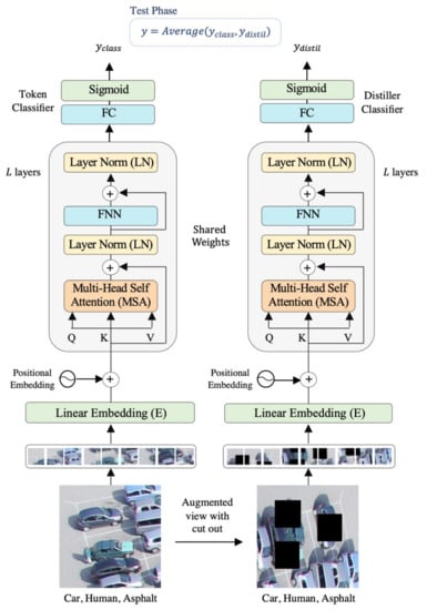
Figure 1. Proposed multi-labeling method.

3.1. Encoder Module

The encoder was adopted from DeiT architecture. It is an improved version of ViT but with the advantage of requiring less data for training. To feed the images into the model, the data are first converted into a sequence of patches. An image $X$ of dimension$h\times w\times c$ is divided into small patches, where $h$, $w,$ and $c$ are the height, the width, and the number of channels of that image, respectively. The patches $X=\left\{x_p^1, x_p^2, \cdots ,x_p^m\right\}$ form a sequence of length $m$, where each patch $x_p$ has the dimension of $p\times p$ and m = $h\times w /p^2$. These patches are analogous to word tokens in the original transformer. The flattened image patches are converted into embeddings by feeding them into a linear embedding layer $E$ to match their dimension to the model dimension $d_{model}$.

Flattening causes the loss of positional information, which is crucial for understanding the image content. To retain this information, each patch embedding is added to its corresponding positional information. The resultant position-aware embeddings are appended with a learnable class token $x_{class}$. The DeiT architecture also introduces another distillation token $x_{distil}$ that is appended along with the class token $x_{class}$ to the patch embeddings (Equation (1)). The two tokens and the patch embeddings interact with each other via the self-attention mechanism.

$$z_0=\left[x_{class}; x_{distil}; x_p^{1}E; x_p^{2}E;\dots ; x_p^{m}E\right]+E_{pos}, E\in {ℝ}^{\left(p^2. c\right)\times d_{model}}, E_{pos}\in {ℝ}^{\left(m+2\right)\times d_{model}}$$

(1)

The encoder consists of a stack of $L$ identical layers; each one is composed of two main blocks: A multi-head self-attention (MSA) block, which is the key component of the model, and a feed-forward network block (FFN). The MSA utilizes the self-attention mechanism to derive long-range dependencies between different patches in the given image. Equation (2). Shows the details of the computations that take place in one self-attention head (SA). First, the input sequence is transformed into three different matrices which are the key $K$, the query $Q$, and the value $V$ using three linear layers $W_i^Q\in {ℝ}^{d_{model}\times d_Q}$, $W_i^K\in {ℝ}^{d_{model}\times d_K}$ and $W_i^V\in {ℝ}^{d_{model}\times d_V}$ for $i=1, 2, \dots h$ where $h$ is the number of heads. The attention map is computed by matching the query matrix against the key matrix using the scaled-dot-product. The output is scaled by the dimension of the key $d_K$and then converted into probabilities by a softmax layer. Finally, the result is multiplied with the value $V$ to get a filtered value matrix which assigns high focus to more important elements.

$$Attention\left(Q, K,V\right)=softmax\left(\frac{Q{K}^T}{\sqrt{d_K}}\right).V$$

(2)

The multi-head self-attention applies this process in parallel using multiple self-attention heads, as shown in Figure 2. Each head has the role to focus on one relationship among the image patches. The outputs of all heads are then concatenated together and passed to a linear layer to project it to the desired dimension, as shown in the following equation:

$$\begin{gathered} MSA\left(Q, K,V\right)=Concat\left(S{A}_1; S{A}_2;\dots S{A}_h\right)W^O,W^O\in {ℝ}^{h.d_K\times d_{model}} \\ S{A}_i=Attention\left(Q{W}_i^Q, K{W}_i^K, V{W}_i^V\right) \end{gathered}$$

(3)

where $W^O$ represents the final projection layer and $W^O, W_i^Q$,$W_i^K$, and$W_i^V$ are all learnable weights. The second main block in the encoder is the feed-forward network (FFN) that is applied after the MSA block. It consists of two fully connected layers with a GELU activation function [33] within them. The two main blocks of the encoder use residual connections and preceded by a layer of normalization (LN) as described in the following equations:

$$z_{ \mathit{l}}^{\prime }=MSA\left(LN\left(z_{\mathit{l}-1}\right)\right)+z_{\mathit{l}-1}, \mathit{l}=1\dots L$$

(4)

$$z_{\mathit{l}}=FFN\left(LN\left(z_{ \mathit{l}}^{\prime }\right)\right)+z_{ \mathit{l}}^{\prime }, \mathit{l}=1\dots L$$

(5)

where $z_L$represents the output of the last encoder layer.

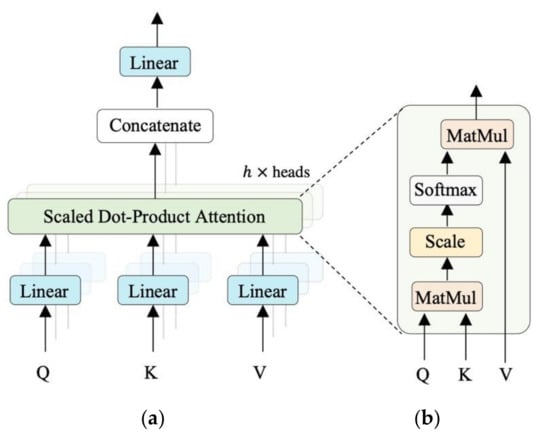
Figure 2. Attention architecture. (a) Multi-head self-attention and (b) Scaled dot-product attention.

Similarly, the augmented view of the image is subdivided into a sequence of patches and fed to the encoder. To generate the second view of the image, we applied different image augmentation techniques. These techniques are ranging from simple transformations such as rotating, scaling, cropping, shifting, and flipping and more advanced techniques such as cutout [34], which randomly masks out one or more patches from the image.

3.2. Classification Layers

On top of the encoder, two external classifiers are connected, the token and distiller classifiers. Each one is composed of a fully connected layer (FC) with a sigmoid activation function to determine the class labels. We feed the first element of the encoder output $z_{ \mathrm{L}}^0$ which represents the classification token to the token classifier.

$$y_{class}=Sigmoid(FC\left(z_{ \mathrm{L}}^0\right)$$

(6)

While the second token $z_{ \mathrm{L}}^1$ which represents the distillation token is passed to the second distiller classifier:

$$y_{distil}=Sigmoid\left(FC\left(z_{ \mathrm{L}}^1\right)\right)$$

(7)

3.3. Network Optimization

To learn the model for the multi-label classification, we formulated the loss as a multiple binary cross-entropy loss, which can be described as:

$${\mathcal{L}}_{BCE}\left(x_{ij}, y_{ij}\right)=-\frac{1}{n}{\displaystyle \sum }_{i=1}^n{\displaystyle \sum }_{j=1}^s{y}_{ij} \log \frac{1}{1+e^{-x_{ij}}}+\left(1-y_{ij}\right)\log \left(1-\frac{1}{1+e^{-x_{ij}}}\right)$$

(8)

where $n$ is the number of training images, $s$ is the number of defined classes, $y_{ij}\in {\left\{0, 1\right\}}^c$ is the ground-truth labels, and $x_{ij}\in \left[0,1\right]$ is the predicted probability. The learning is performed by minimizing a total loss consisting of two terms given by the following equation:

$${\mathcal{L}}_{total}={\mathcal{L}}_{BCE}\left(y_{class}, y_g\right)+{\mathcal{L}}_{BCE}\left(y_{distil}, y_g\right)$$

(9)

where ${\mathcal{L}}_{\mathrm{BCE}}$ is the binary cross-entropy loss defined in Equation (8), $y_g$ is the ground-truth labels, and $y_{class}$ and $y_{distil}$ represent the outputs of the token and distiller classifiers, respectively. Afterward, at the test time, when a model is given an image, the outputs of the two classifiers are averaged and considered as the predicted class labels (Algorithm 1).

$$y=(y_{class}+y_{distil})/2$$

(10)

3.4. Algorithm

In the following, we provide the main steps for training the model:

Algorithm 1 Multi-Label Classification.

Input: Training set of n UAV images $\mathcal{D}={\left\{X_{\mathrm{i}},Y_{\mathrm{i}}\right\}}_{i=1}^n$ and their corresponding ground-truth labels. Output: The predicted class labels of the test set 1. Set the model parameters: Mini-batch size $b$: 5$0$; Patch size $p$: 16; Optimizer: Adam, learning rate: 0.0003; Number of iterations: 20; Image size:$224$ 2. Set the number of mini-batches as: $n_b=n/b$; 3. For iteration = 1: Number of iterations; 3.1. For batch $=1: n_b$; Pick a batch from the training set; Generate a batch of augmented images; Feed the batch of the original images to the encoder; Feed the batch of augmented images to the encoder; Feed the classification token to the token classifier and the distiller token to the distiller classifier; Calculate the loss defined in Equation (9); Backpropagate the loss; Update the model parameters. 4. Feed the test images to the model; 5. The predicted labels are the average of the two outputs $y_{token}$and $y_{distiller}$.

4. Experimental Results

4.1. Data Set Description

In our experiments, two multi-label UAV datasets were used for evaluation: the Trento multi-label dataset and the Civezzano multi-label dataset. Some information about these datasets is summarized in Table 1, and samples from each dataset are shown in Figure 3.

Table 1. Information about multi-label UAV datasets.

	No. of Classes	No. of Images	Spatial Resolution (cm)	Spectral Resolution	Image Size
Trento	13	3415	2	RGB	224 × 224
Civezzano	14	3415	2	RGB	224 × 224

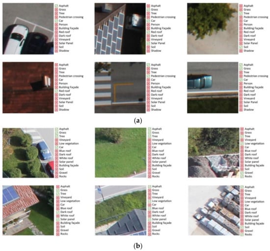
Figure 3. Sample images. (a) Trento and (b) Civezzano multi-label datasets (green color indicates the presence of the class while red color indicates the absence of the class in the image).

The Trento dataset consisted of UAV imagery acquired over the faculty of science of the University of Trento in Italy on 3 October 2011. The dataset was obtained using nadir acquisition performed with a Canon EOS 550D camera with a CMOS APS-C 18-megapixels sensor. The images of the dataset had the dimensions 224 × 224 pixels, a ground sampling resolution of approximately 2 cm, and RGB spectral channels. The multi-label version was built upon the Trento single-label dataset, and it had 3415 images in total; 1000 were selected for training, and 2415 were kept for testing. The dataset was defined with 13 distinct class labels. These labels were: Asphalt, Grass, Tree, Pedestrian Crossing, Car, Person, Building Façade, Red roof, Dark roof, Vineyard, Solar Panel, Soil, and Shadow.

The Civezzano multi-label dataset was a UAV dataset that has been acquired near the city of Civezzano in Italy, on 17 October 2012, at different off-nadir viewing angles. The acquisition was performed using a Canon EOS 550D picture camera equipped with a CMOS APS-C 18-megapixels sensor. Each UAV image had three channels (RGB) and a spatial resolution of 2 cm. The Civezzano dataset contained 3415 images, 1000 for training and 2415 for testing. The dataset’s images were assigned to different 14 class labels: Asphalt, Grass, Tree, Vineyard, Low Vegetation, Car, Blue roof, White roof, Dark roof, Solar Panel, Building façade, Soil, Gravel, and Rocks.

4.2. Evaluation Metrics

To quantitatively validate the proposed methodology and compare our results to other state-of-the-art methods, we calculated the following metrics: specificity (Sp), recall (Re), precision (Pr), average (Avg), F1-score (F1), F2-score (F2), mean average precision (mAP), ranking loss (RL), and Hamming loss (HL). The definitions of these metrics are given as below:

• $Specificity=\frac{TN}{TN+FP}$, $Recall=\frac{TP}{TP+FN}$, $Precision=\frac{TP}{TP+FP}$, where TP, FP, TN, FN are the number of true positives, false positives, true negatives, and false negatives;
• Average (Avg): is the average of specificity and recall;
• $Fscore=\frac{\left(1+{\beta }^2 \right) \left(Precision\times Recall\right)}{{\beta }^2 \left(Precision+Recall\right)}$, where $\beta$ has the value of 1 for F1-score and 2 for the F2-score;
• Mean average precision (mAP): is the mean of average precisions for each class;
• Ranking loss (RL): is the average number of incorrectly ordered pairs of labels;
• Hamming loss (HL) is the fraction of incorrectly predicted labels to the total number of labels.

4.3. Experimental Setup

For the encoder architecture, we adopted the DeiT-Base model following the implementation in [28]. The model had 12 layers, where each layer contained 12 parallel self-attention heads. The model used an image size of 224 × 224 and split each image into patches of size of 16 × 16. The resulted sequence length is 196 tokens. This sequence was then mapped to model embedding dimension of size 768. To generate the augmented version of the image, we applied horizontal and vertical flipping with a probability of 0.5, a rotation with 25° and a cutout technique with a number of patches to cut out from the image is eight, and a cutout region of 50 × 50 pixels.

We used a model pre-trained on ImageNet dataset and fine-tuned it for 20 epochs on the UAV dataset with a mini-batch of size 50. We optimized the model with the Adam method and set the learning rate to 0.0003. During training, we learned the network in two directions. In the first direction, both the query and the key were generated from the original image, while the value is generated from the augmented image. In the second direction, the query and the key are generated from the augmented image, and the value was generated from the original image.

We implemented all the experiments in Python with the PyTorch library using a PC workstation having a Central Processing Unit (CPU) Core i9 processor with a speed of 2.9 GHz, 32 GB of memory, and a Graphical Processing Unit (GPU) with 11 GB GDDR5X memory.

4.4. Results

4.4.1. Experiment 1: The Effect of Data Augmentation

In the first set of experiments, we tested the effect of using data augmentation on the classification results. Experimental results on single-label scene classification have shown that using a combination of data augmentation techniques can improve the classification results [25]. Therefore, we augmented the dataset with additional samples using random flipping, rotations, and cutout during training. The results of the experiments are reported in Table 2 and Table 3 for the Trento and Civezzano datasets, respectively. The results indicated that the performance could be remarkably improved through the use of image augmentation techniques. Specifically, for the Trento dataset it increased the F1-score by ~7%, the F2-score by ~9%, the average by ~3%, and the mean average precision by ~10%. The results also showed that using data augmentation reduced the hamming loss from 8.87 to 6.75 and the ranking loss from 34.10 to 28.46. In contrast, data augmenting increased the time needed for training the model, which was expected as the model is being trained with more samples. For the Civezzano dataset, the use of data augmentation increases the F1-score by ~3%, the F2-score by ~7%, and the mean average precision by ~6%. However, results show that augmenting data has no effect on the average and has a negative effect on the training time. In general, and as the results on the two datasets suggest, using data augmentation for UAV image multi-labeling could significantly improve the classification results, with a slight increase in the training time.

Table 2. Results of Trento multi-label dataset.

	Sp	Re	Pr	F1	F2	Avg	mAP	HL	RL	Time
With Augmentation	97.57	68.33	82.98	74.95	79.57	82.95	61.38	6.75	28.46	4224
Without Augmentation	95.84	63.91	72.73	68.03	70.78	79.88	51.81	8.87	34.10	3550

Table 3. Results of Civezzano multi-label dataset.

	Sp	Re	Pr	F1	F2	Avg	mAP	HL	RL	Time
With Augmentation	97.91	76.77	86.43	81.32	84.31	87.34	69.79	5.20	15.42	4156
Without Augmentation	95.80	78.90	76.50	77.68	76.97	87.35	63.48	6.69	20.64	3353

4.4.2. Experiment 2: The Role of Encoder’s Layers

To assess the role of each layer in the encoder, we repeated the experiments with a different number of encoder layers. Table 4 and Figure 4 summarize the experimental results of using a different number of layers on the Trento dataset, and Table 5 and Figure 5 show the results on the Civezzano dataset. In general, better results were obtained with a higher number of layers. However, adding more layers increased the complexity of the encoder architecture and hence, increased the time required to train the model. Figure 4 and Figure 5 show visually that performance started to plateau after layer 10 in both datasets. Therefore, for UAV multi-labeling, an encoder with ten layers would be sufficient to achieve good results.

Table 4. Results of the Trento multi-label dataset.

Number of Layers	Sp	Re	Pr	F1	F2	Avg	mAP	HL	RL	Time (Seconds)
1	93.55	53.73	59.07	56.27	57.92	73.64	38.57	12.33	45.31	629
2	95.06	63.14	68.90	65.89	67.67	79.10	48.95	9.65	34.48	932
3	94.42	63.03	66.20	64.57	65.54	78.73	47.18	10.21	35.58	1203
4	94.79	55.89	65.00	60.10	62.95	75.34	42.84	10.96	41.30	1608
5	95.36	56.06	67.68	61.33	64.99	75.71	44.43	10.44	41.24	1941
6	95.40	60.46	69.48	64.66	67.47	77.93	47.85	9.76	37.29	2482
7	95.45	59.01	69.20	63.70	66.89	77.23	46.89	9.93	38.78	2773
8	96.60	57.77	74.62	65.12	70.50	77.18	49.34	9.14	39.80	3023
9	97.38	59.36	79.72	68.05	74.60	78.37	53.33	8.23	37.24	3347
10	97.57	68.59	83.02	75.12	79.68	83.08	61.59	6.70	28.65	3630
11	97.47	63.18	81.25	71.08	76.85	80.33	56.77	7.59	33.25	3991
12	97.57	68.33	82.98	74.95	79.57	82.95	61.38	6.75	28.46	4224

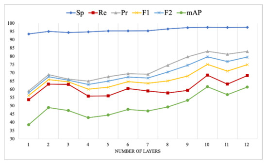
Figure 4. Results of our model on the Trento multi-label dataset.

Table 5. Results of the Civezzano multi-label dataset.

Number of Layers	Sp	Re	Pr	F1	F2	Avg	mAP	HL	RL	Time (Seconds)
1	96.25	69.14	76.14	72.47	74.63	82.69	57.20	7.75	28.14	731
2	95.93	73.15	75.96	74.40	75.17	83.54	59.33	7.43	24.65	1022
3	96.04	73.95	76.41	75.16	75.91	85.00	60.35	7.21	23.98	1288
4	95.92	71.60	75.22	73.37	74.47	83.76	58.05	7.67	26.76	1673
5	96.80	73.11	79.82	76.32	78.38	84.95	62.33	6.70	24.66	2019
6	95.78	76.17	75.78	75.97	75.86	85.98	61.24	7.11	23.00	2353
7	96.89	74.59	80.58	77.47	79.31	85.74	63.85	6.40	23.53	2556
8	96.41	77.96	78.97	78.46	78.76	87.18	64.81	6.32	21.54	2835
9	97.12	77.98	82.40	80.13	81.48	87.55	67.50	5.71	20.87	3036
10	97.14	80.54	82.99	81.75	82.49	88.84	69.71	5.31	18.67	3347
11	97.49	78.88	84.50	81.59	83.31	88.19	69.77	5.25	18.85	3769
12	97.91	76.77	86.43	81.32	84.31	87.34	69.79	5.20	15.42	4156

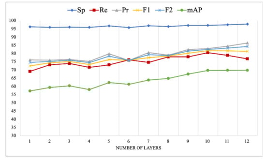
Figure 5. Results of our model on the Civezzano multi-label dataset.

In detail, the results of the Trento dataset showed a consistent improvement in all metrics as the number of layers increased. However, the performance started to decrease after the tenth layer. At the same time, the results of the Civezzano dataset show a slight decrease in few metrics such as the recall, the F1-score, and the average after layer 10.

We further visualized the attention heat map learned by each layer of our model. Figure 6 and Figure 7 show the attention heat maps generated by the first, sixth, and last layers of the encoder for the two UAV datasets. The red color in the attention heat maps highlights the areas with maximum attention weight, while the blue color represents the areas with lower attention weight. The attention heat maps clearly show that the self-attention component in our model was able to capture the long-range relations across the entire scene. Moreover, the attention heat maps show that as the number of layers increased, the model improved its ability to focus on the regions corresponding to objects existing in the scene. This can be highly noticed in the initial layers from one to six, which played a key role in highlighting the discriminative regions. In contrast, the later layers of the encoder (i.e., from 7 to 12) had the role of refining the attention heat maps resulted from the previous layers and detecting the details of the objects.

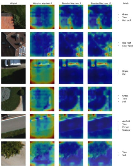
Figure 6. Attention heat maps generated by the first, sixth, and last layers of the encoder for classifying different samples from Trento multi-label datasets.

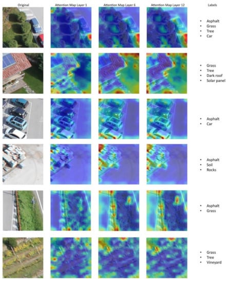
Figure 7. Attention heat maps generated by the first, sixth, and last layers of the encoder for classifying different samples from Civezzano multi-label datasets.

5. Discussion

In order to show the benefits of our multi-label classification method, we compared it against several state-of-the-art methods. We mainly choose to compare it with conditional random field method (Full-ML-CRF) [9], BOVW with color and shape representation (HCB) [31], pre-trained models with different classifiers including, SVM, multi-label regression layer (MLR), radial basis function (RBF), radial basis function neural networks (RBFNN), and multi-labeling layer (ML) [31], CNN with the max-margin loss [9], and CNN-LSTM methods with attention [14].

Table 6 shows the results of the comparison on the Trento dataset. It can be seen that our approach achieves the highest values on three metrics, namely, the specificity, the precision, and the mean average precision, with the values of 97.57%, 82.98%, and 61.38%, respectively. Furthermore, our model showed a Hamming loss of 6.75, which was lower than other methods. However, in terms of average metric, our approach achieved the second-best results, which was only 0.64% lower than the next best method, and achieved the second-lowest ranking loss. However, in terms of recall, the achieved result was low compared to other techniques.

Table 6. Results of the Trento multi-label dataset.

Method	Sp	Re	Pr	F1	F2	Avg	mAP	HL	RL
Full-ML-CRF [9]	82.20	70.30				76.20
HCB [31]	92.20	60.70				76.40
GoogLeNet (MLR)	92.70	60.80				76.80
AlexNet (MLR)	94.50	60.40				77.50
GoogLeNet (RBFNN)	95.40	63.10				79.30
AlexNet (RBFNN)	96.20	60.60				78.40
GoogLeNet-SVM (linear)	96.40	59.00				77.70
GoogLeNet-SVM(RBF)	96.30	58.60				77.50
AlexNet-SVM (linear)	95.50	54.50				75.00
AlexNet-SVM(RBF)	95.70	52.50				74.10
GoogLeNet-RBFNN(ML)	90.30	75.10				82.70
AlexNet- RBFNN(ML)	93.00	70.50				81.80
CNN-RBFNN [11]	92.60	68.60				80.60
CNN-MaxMargin loss [35]	95.44	61.32	71.02			78.38	49.50	9.80	35.72
CNN-Softmax loss	92.04	69.49	61.37			80.77	47.34	11.42	29.89
CNN-LSTM	93.81	64.19	65.36			79.00	47.46	10.74	33.62
LSTM+CNN +Spatial Attention	93.86	66.49	66.43			80.17	49.27	10.30	31.69
Deep Attention CNN-LSTM [14]	94.01	73.17	68.98			83.59	54.60	9.19	25.33
Our approach	97.57	68.33	82.98	74.95	79.57	82.95	61.38	6.75	28.46

The comparative results on the Civezzano dataset are shown in Table 7. As can be seen, our method achieved the best results with a specificity of 97.91%, precision of 86.43%, average of 87.34%, and mean average precision of 69.79%, 5.20 Hamming loss, and a 15.42 ranking loss. Our method outperformed all the existing UAV multi-label classification approaches in all metrics except Recall, in which it achieved the second-best result, which was only 1.53% lower compared to the Deep Attention CNN-LSTM [14].

Table 7. Results of the Civezzano multi-label dataset.

Method	Sp	Re	Pr	F1	F2	Avg	mAP	HL	RL
Full-ML-CRF [9]	90.80	75.90				83.40
HCB [31]	91.90	61.40				76.60
GoogLeNet(MLR)	92.90	58.70				75.80
AlexNet(MLR)	94.00	58.00				76.00
GoogLeNet-Logistic regression [11]	92.90	58.70
AlexNet-Logistic regression [11]	94.00	58.00
GoogLeNet-RBFNN [11]	96.10	58.70				77.40
AlexNet-RBFNN [11]	95.40	58.30				76.90
GoogLeNet-SVM (linear) [11]	96.10	58.10				77.10
GoogLeNet-SVM(RBF) [11]	95.10	53.60				74.40
AlexNet-SVM (linear) [11]	95.20	52.30				73.70
AlexNet-SVM(RBF) [11]	95.20	52.30				73.80
GoogLeNet-RBFNN(multi-label layer) [11]	92.60	68.60				80.60
AlexNet- RBFNN(multi-label layer) [11]	93.20	66.10				79.70
CNN-MaxMargin loss [35]	95.70	70.79	74.71			83.33	57.44	8.53	26.51
CNN-Softmax loss	95.22	70.37	72.52			82.79	55.53	8.54	27.31
CNN-LSTM	94.60	69.40	69.72			82.00	53.03	9.22	28.93
LSTM+CNN +Spatial Attention	96.78	69.51	79.45			83.14	59.86	7.35	27.11
Deep Attention CNN-LSTM [14]	95.56	78.30	75.94			86.93	62.76	7.06	21.18
Full-ML-CRF [9]	90.80	75.90				83.40
SSSVM [12]	91.57	76.69
Our approach	97.91	76.77	86.43	81.32	84.31	87.34	69.79	5.20	15.42

6. Conclusions

In this work, we proposed a multi-label classification method for high-resolution UAV imagery. The proposed method utilized the self-attention mechanism in the vision transformer to derive the correlation between different objects within the scene. Moreover, we mounted a cross-attention module on the top of our model to detect the cross-correlation between the image and its augmented view. We showed experimentally that using vision transformers in multi-label classification can help in improving the accuracy when combined with different data augmentation techniques. We conducted several experiments on two UAV datasets, and the results demonstrated the effectiveness of the proposed method compared to state-of-the-art methods.

References

- Yao, H.; Qin, R.; Chen, X. Unmanned Aerial Vehicle for Remote Sensing Applications—A Review. Remote Sens. 2019, 11, 1443. [Google Scholar] [CrossRef]
- Bashmal, L.; Bazi, Y.; AlHichri, H.; AlRahhal, M.; Ammour, N.; Alajlan, N. Siamese-GAN: Learning Invariant Representations for Aerial Vehicle Image Categorization. Remote Sens. 2018, 10, 351. [Google Scholar] [CrossRef]
- Hossain, M.D.; Chen, D. Segmentation for Object-Based Image Analysis (OBIA): A Review of Algorithms and Challenges from Remote Sensing Perspective. ISPRS J. Photogramm. Remote Sens. 2019, 150, 115–134. [Google Scholar] [CrossRef]
- Li, K.; Wan, G.; Cheng, G.; Meng, L.; Han, J. Object Detection in Optical Remote Sensing Images: A Survey and a New Benchmark. ISPRS J. Photogramm. Remote Sens. 2020, 159, 296–307. [Google Scholar] [CrossRef]
- Chaudhuri, B.; Demir, B.; Chaudhuri, S.; Bruzzone, L. Multilabel Remote Sensing Image Retrieval Using a Semisupervised Graph-Theoretic Method. IEEE Trans. Geosci. Remote Sens. 2018, 56, 1144–1158. [Google Scholar] [CrossRef]
- Aksoy, A.K.; Ravanbakhsh, M.; Kreuziger, T.; Demir, B. CCML: A Novel Collaborative Learning Model for Classification of Remote Sensing Images with Noisy Multi-Labels. arXiv 2020, arXiv:2012.10715. [Google Scholar]
- Li, Y.; Chen, R.; Zhang, Y.; Zhang, M.; Chen, L. Multi-Label Remote Sensing Image Scene Classification by Combining a Convolutional Neural Network and a Graph Neural Network. Remote Sens. 2020, 12, 4003. [Google Scholar] [CrossRef]
- Diao, Y.; Chen, J.; Qian, Y. Multi-Label Remote Sensing Image Classification with Deformable Convolutions and Graph Neural Networks. In Proceedings of the IGARSS 2020-2020 IEEE International Geoscience and Remote Sensing Symposium, Waikoloa, HI, USA, 26 September 2020; pp. 521–524. [Google Scholar]
- Zeggada, A.; Benbraika, S.; Melgani, F.; Mokhtari, Z. Multilabel Conditional Random Field Classification for UAV Images. IEEE Geosci. Remote Sens. Lett. 2018, 15, 399–403. [Google Scholar] [CrossRef]
- Karalas, K.; Tsagkatakis, G.; Zervakis, M.; Tsakalides, P. Land Classification Using Remotely Sensed Data: Going Multilabel. IEEE Trans. Geosci. Remote Sens. 2016, 54, 3548–3563. [Google Scholar] [CrossRef]
- Zeggada, A.; Melgani, F.; Bazi, Y. A Deep Learning Approach to UAV Image Multilabeling. IEEE Geosci. Remote Sens. Lett. 2017, 14, 694–698. [Google Scholar] [CrossRef]
- Koda, S.; Zeggada, A.; Melgani, F.; Nishii, R. Spatial and Structured SVM for Multilabel Image Classification. IEEE Trans. Geosci. Remote Sens. 2018, 1–13. [Google Scholar] [CrossRef]
- Stivaktakis, R.; Tsagkatakis, G.; Tsakalides, P. Deep Learning for Multilabel Land Cover Scene Categorization Using Data Augmentation. IEEE Geosci. Remote Sens. Lett. 2019, 16, 1031–1035. [Google Scholar] [CrossRef]
- Alshehri, A.; Bazi, Y.; Ammour, N.; Almubarak, H.; Alajlan, N. Deep Attention Neural Network for Multi-Label Classification in Unmanned Aerial Vehicle Imagery. IEEE Access 2019, 7, 119873–119880. [Google Scholar] [CrossRef]
- Ji, J.; Jing, W.; Chen, G.; Lin, J.; Song, H. Multi-Label Remote Sensing Image Classification with Latent Semantic Dependencies. Remote Sens. 2020, 12, 1110. [Google Scholar] [CrossRef]
- Hua, Y.; Mou, L.; Zhu, X.X. Recurrently Exploring Class-Wise Attention in a Hybrid Convolutional and Bidirectional LSTM Network for Multi-Label Aerial Image Classification. ISPRS J. Photogramm. Remote Sens. 2019, 149, 188–199. [Google Scholar] [CrossRef] [PubMed]
- Sumbul, G.; Demir, B. A Deep Multi-Attention Driven Approach for Multi-Label Remote Sensing Image Classification. IEEE Access 2020, 8, 95934–95946. [Google Scholar] [CrossRef]
- Kang, J.; Fernandez-Beltran, R.; Hong, D.; Chanussot, J.; Plaza, A. Graph Relation Network: Modeling Relations Between Scenes for Multilabel Remote-Sensing Image Classification and Retrieval. IEEE Trans. Geosci. Remote Sens. 2020, 1–15. [Google Scholar] [CrossRef]
- Tan, Q.; Liu, Y.; Chen, X.; Yu, G. Multi-Label Classification Based on Low Rank Representation for Image Annotation. Remote Sens. 2017, 9, 109. [Google Scholar] [CrossRef]
- Hua, Y.; Mou, L.; Zhu, X.X. Relation Network for Multilabel Aerial Image Classification. IEEE Trans. Geosci. Remote Sens. 2020, 58, 4558–4572. [Google Scholar] [CrossRef]
- Bilen, H.; Vedaldi, A. Weakly Supervised Deep Detection Networks. In Proceedings of the 2016 IEEE Conference on Computer Vision and Pattern Recognition (CVPR), Las Vegas, NV, USA, June 2016; pp. 2846–2854. [Google Scholar]
- Tang, P.; Wang, X.; Wang, A.; Yan, Y.; Liu, W.; Huang, J.; Yuille, A. Weakly Supervised Region Proposal Network and Object Detection. In Computer Vision—ECCV 2018; Lecture Notes in Computer Science; Ferrari, V., Hebert, M., Sminchisescu, C., Weiss, Y., Eds.; Springer International Publishing: Cham, Switzerland, 2018; Volume 11215, pp. 370–386. ISBN 978-3-030-01251-9. [Google Scholar]
- Ge, W.; Yang, S.; Yu, Y. Multi-Evidence Filtering and Fusion for Multi-Label Classification, Object Detection and Semantic Segmentation Based on Weakly Supervised Learning. In Proceedings of the 2018 IEEE/CVF Conference on Computer Vision and Pattern Recognition, Salt Lake City, UT, USA, 18–23 June 2018; pp. 1277–1286. [Google Scholar]
- Dosovitskiy, A.; Beyer, L.; Kolesnikov, A.; Weissenborn, D.; Zhai, X.; Unterthiner, T.; Dehghani, M.; Minderer, M.; Heigold, G.; Gelly, S.; et al. An Image Is Worth 16 × 16 Words: Transformers for Image Recognition at Scale. arXiv 2020, arXiv:2010.11929 [cs]. [Google Scholar]
- Bazi, Y.; Bashmal, L.; Rahhal, M.M.A.; Dayil, R.A.; Ajlan, N.A. Vision Transformers for Remote Sensing Image Classification. Remote Sens. 2021, 13, 516. [Google Scholar] [CrossRef]
- He, J.; Zhao, L.; Yang, H.; Zhang, M.; Li, W. HSI-BERT: Hyperspectral Image Classification Using the Bidirectional Encoder Representation From Transformers. IEEE Trans. Geosci. Remote Sens. 2020, 58, 165–178. [Google Scholar] [CrossRef]
- Vaswani, A.; Shazeer, N.; Parmar, N.; Uszkoreit, J.; Jones, L.; Gomez, A.N.; Kaiser, Ł.; Polosukhin, I. Attention Is All You Need. In Proceedings of the Advances in Neural Information Processing Systems, Long Beach, CA, USA, 4–9 December 2017; pp. 5998–6008. [Google Scholar]
- Touvron, H.; Cord, M.; Douze, M.; Massa, F.; Sablayrolles, A.; Jégou, H. Training Data-Efficient Image Transformers & Distillation through Attention. arXiv 2020, arXiv:2012.12877. [Google Scholar]
- Hinton, G.; Vinyals, O.; Dean, J. Distilling the Knowledge in a Neural Network. arXiv 2015, arXiv:1503.02531. [Google Scholar]
- Cheng, G.; Li, Z.; Yao, X.; Guo, L.; Wei, Z. Remote Sensing Image Scene Classification Using Bag of Convolutional Features. IEEE Geosci. Remote Sens. Lett. 2017, 14, 1735–1739. [Google Scholar] [CrossRef]
- Moranduzzo, T.; Melgani, F.; Mekhalfi, M.L.; Bazi, Y.; Alajlan, N. Multiclass Coarse Analysis for UAV Imagery. IEEE Trans. Geosci. Remote Sens. 2015, 53, 6394–6406. [Google Scholar] [CrossRef]
- Zhu, P.; Tan, Y.; Zhang, L.; Wang, Y.; Mei, J.; Liu, H.; Wu, M. Deep Learning for Multilabel Remote Sensing Image Annotation With Dual-Level Semantic Concepts. IEEE Trans. Geosci. Remote Sens. 2020, 58, 4047–4060. [Google Scholar] [CrossRef]
- Hendrycks, D.; Gimpel, K. Gaussian Error Linear Units (GELUs). arXiv 2020, arXiv:1606.08415. [Google Scholar]
- DeVries, T.; Taylor, G.W. Improved Regularization of Convolutional Neural Networks with Cutout. arXiv 2017, arXiv:1708.04552. [Google Scholar]
- Shi, W.; Gong, Y.; Tao, X.; Zheng, N. Training DCNN by Combining Max-Margin, Max-Correlation Objectives, and Correntropy Loss for Multilabel Image Classification. IEEE Trans. Neural. Netw. Learn. Syst. 2017, 1–13. [Google Scholar] [CrossRef]
Publisher’s Note: MDPI stays neutral with regard to jurisdictional claims in published maps and institutional affiliations. |
© 2021 by the authors. Licensee MDPI, Basel, Switzerland. This article is an open access article distributed under the terms and conditions of the Creative Commons Attribution (CC BY) license (https://creativecommons.org/licenses/by/4.0/).