
An Efficient Library for Reliability Block Diagram Evaluation


Abstract
:1. Introduction
- Combinatorial models: they allow to efficiently evaluate reliability under the strong assumption of statistically independent components [3,4]. These models include Reliability Block Diagrams (RBDs) [5,6], Fault Trees (FTs) [7,8], Reliability Graphs (RGs) [9,10] and Fault Trees with Repeated Events (FTREs) [8,11].
- State-space based models: they allow for the modeling of several dependencies among failures, including statistical, time and space dependency, at the cost of a difficult tractability due to the state-space explosion [3,4]. These models include Continuous Time Markov Chains (CTMCs) [12,13], Stochastic Petri Nets (SPNs), Generalized Stochastic Petri Nets (GSPNs) and Stochastic Time Petri Nets (STPNs) [14,15,16,17], Stochastic Reward Nets (SRNs) [18,19] and Stochastic Activity Networks (SANs) [20,21].
Context and Motivation
- To be highly optimized.
- To allow the resolution of RBD basic blocks (excluding singleton given its trivial formula).
- To allow the reliability computation of an RBD basic block in a time interval.
- To be available as a free software.
- To be available for the most common Operating Systems (OS), i.e., Windows, Mac OS and Linux.
- RBDTool: this open-source and multiplatform tool allows the definition of RBD models and it provides support for their quantitative analysis [37].
- Edraw Block Diagram: this commercial tool allows the definition of RBD models [38].
- Reliability Workbench: this commercial tool allows the definition and analysis of scalable RBD models through the usage of submodels. Furthermore, it supports the minimal cut-set analysis of the RBD model [39].
- Relyence RBD: this commercial tool has features comparable with Reliability Workbench [40].
- SHARPE: the Symbolic Hierarchical Automated Reliability and Performance Evaluator (SHARPE) tool is a general hierarchical modeling tool that analyzes stochastic models of reliability, availability, performance and performability [41,42]. This tool allows the definition of hierarchical reliability models with several formalisms, including RBDs, and it supports the time-dependent reliability analysis.
2. Reliability Block Diagrams
- 1.
- The modeled system, as well as each component, has only two states, i.e., success and failure.
- 2.
- The RBD represents the success state of the modeled system through the usage of success paths, i.e., the connections of the success states of its components.
- 3.
- The system components are statistically independent. Under this assumption, the probability of failure of the block A, , is not related with the probability of failure of the block such that .
2.1. Basic Blocks
- Singleton. This block is the simplest one and it is composed by a single component. The block state is equal to success if and only if the component is in success state. An example is a stand-alone Power Supply.
- Series. This block is composed by N components. The block state is equal to success if and only if all the components are in success state. An example is a 2-out-of-2 computing system (2oo2).
- Parallel. This block is composed by N components. The block state is equal to success if and only if at least one component is in success state, or, in other terms, the block state is equal to failure if and only if all the components are in the failure state. An example is a redundant Power Supply system with current sharing.
- K-out-of-N(KooN). This block is composed by N components. The block state is equal to success if and only if at least K components out of N are in success state. An example is a 2-out-of-3 computing system (2oo3).
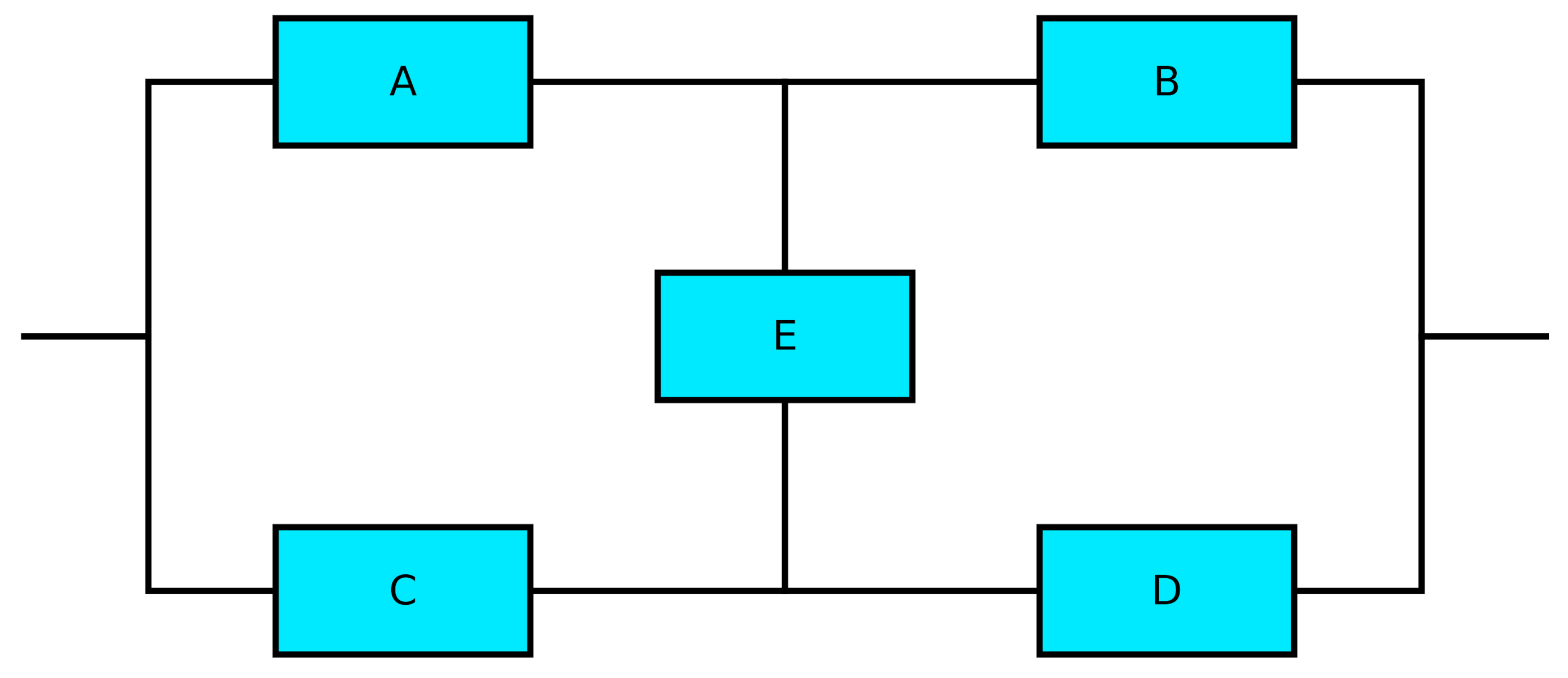
- Bridge. This block is composed by 5 components arranged as shown in Figure 3. The block state is equal to success if at least one of the four following conditions is satisfied:
- 1.
- Components A and B are correctly operating.
- 2.
- Components C and D are correctly operating.
- 3.
- Components A, E and D are correctly operating.
- 4.
- Components C, E and B are correctly operating.
An example is a network infrastructure.
2.2. Quantitative Evaluation Using RBDs
2.2.1. Quantitative Evaluation: General Formulas
- Series. The probability of success of the series block is computed as:
- Parallel. The probability of failure of the parallel block is computed as:The probability of success of the parallel block is thus computed as:
- K-out-of-N(KooN). In order to compute the probability of success of a KooN block, we can use one of the following approaches:
- 1.
- Let be the j-th unique combination of i out of N components correctly working. For a given couple , the number of unique combinations is equal to the binomial coefficient . We define as the specific realization of one of the possible system states for which i components out of N are correctly working while the other have failed: the exact set of the working components is selected through the usage of unique combination . Its probability of occurrence is:The state of a KooN block is equal to success if and only if the current system state is satisfied by one path of at least K working components. The probability of success of the KooN block can be defined as:
- 2.
- Observe that the probability of success of a system with 0 or more components out of I in success state is equal to 1 and observe that the probability of success of a system with J or more components out of I with in success state is equal to 0. A recursive approach for evaluating the probability of success of a KooN system is derived by conditioning on the state of the N-th component [3]. The N-th component can assume only two states, success with probability and failed with probability . Let us assume that the N-th component is correctly working: for a KooN system to be correctly operating, we need at least working components out of the remaining . If, on the other hand, the N-th component is failed, we need at least K working components out of the remaining in order to have a correctly operating KooN system. The probability of success of a KooN block can then be recursively computed as:
- Bridge. In order to compute the probability of success of a bridge block, we apply the same decompositional approach used in the second set of formulas to compute the probability of success of a KooN block. Let us analyze the bridge block by conditioning the status of component E. If E is failed, the state of the block is equal to success if either A and B or C and D are correctly operating, i.e., if the parallel of two series A, B and C, D is satisfied. The probability of occurrence of this first event is equal to the probability of failure of E. On the other hand, if E is correctly operating, the state of the block is equal to success if at least one component between A and C is correctly operating and if at least one component between B and D is correctly operating, i.e., if the series of two parallel A, C and B, D is satisfied. The probability of occurrence of this second event is equal to the probability of success of E. The probability of success of a bridge block can then be computed through the formula:
2.2.2. Quantitative Evaluation: Identical Components’ Formulas
- Series. By substituting with p in Equation (2), we can compute the simplified probability of success of the series block as:
- Parallel. By substituting with p in Equation (4), we can compute the simplified probability of success of the parallel block as:
- Bridge. By substituting to with p and to with q in (8), we obtain simplified probability of success of the bridge block as:
2.3. Reliability Evaluation Using RBDs
3. RBD Computation Library-librbd
- To be highly optimized;
- To support the most common OSes, i.e., Windows, Mac OS and Linux;
- To support the numerical computation of the reliability curve for all RBD basic blocks;
- To be available as a free software.
- Number N of components within the block;
- Number T of temporal instants to be analyzed;
- Reliability values R for the modeled components over the requested time instants.
3.1. Design
3.1.1. Optimizations for KooN Computation
| Algorithm 1: Computation of RBD KooN block with generic components. |
| Input: Reliability of each component Result: Reliability R of KooN block begin ; ; if then for do ; if then ; for do for do ; else ; else for do ; if then ; for do for do ; else ; |
| Algorithm 2: Auxiliary functions for computation of RBD KooN block with generic components. |
| Input: Reliability of each component Input: j-th combination of iooN components Function ReliabilityStep(N, i, j) ; for do if then ; else ; return ; Function ReliabilityRecursive(i, j) if then return 1; if then return 0; return ; |
| Algorithm 3: Computation of RBD KooN block with identical components. |
| Input: Reliability of each component Result: Reliability R of KooN block begin if then ; for do ; else ; for do ; |
3.1.2. Symmetric Multi-Processing (SMP)
- Download pthreads-win32, a freely available library which implements a large subset of the POSIX standard threads related API for Windows [49]. After pthreads-win32 has been downloaded, it is possible to use the desired IDE and Compiler (e.g., Visual Studio).
- Download and install Cygwin, a freely available environment (i.e., tools and libraries) which provides a large collection of GNU and Open Source tools, including GCC, and a substantial POSIX API functionality, including pthreads-win32 [50].
3.2. Validation
3.3. librbd Usage
3.3.1. API for Generic Components
- int rbdSeriesGeneric(double *R, double *O, unsigned char N, unsigned int T)
- int rbdParallelGeneric(double *R, double *O, unsigned char N, unsigned int T)
- int rbdKooNGeneric(double *R, double *O, unsigned char N, unsigned char K, unsigned int T)
- int rbdBridgeGeneric(double *R, double *O, unsigned char N, unsigned int T)
- N: the number of components inside the block. Note that, for the bridge block, the number of components must be equal to 5.
- K: the minimum number of components inside the block. Note that this parameter is available for KooN blocks.
- T: the number of time instants over which the reliability curve is computed.
- R: the reliability curves for the input components. Since this is the generic components case, this parameter underlies an N × T matrix.
- O: the computed reliability curve, returned as an array of T elements.
3.3.2. API for Identical Components
- int rbdSeriesIdentical(double *R, double *O, unsigned char N, unsigned int T)
- int rbdParallelIdentical(double *R, double *O, unsigned char N, unsigned int T)
- int rbdKooNIdentical(double *R, double *O, unsigned char N, unsigned char K, unsigned int T)
- int rbdBridgeIdentical(double *R, double *O, unsigned char N, unsigned int T)
- N: the number of components inside the block. Note that, for the bridge block, the number of components must be equal to 5.
- K: the minimum number of components inside the block. Note that this parameter is available for KooN blocks.
- T: the number of time instants over which the reliability curve is computed.
- R: the reliability curves for the input components. Since this is the identical components case, this parameter underlies an array of T elements.
- O: the computed reliability curve, returned as an array of T elements.
3.3.3. Example of librbd Usage
| Listing 1: Example of librbd usage. |
| #include <stdio.h> #include <string.h> #include “rbd.h” /* Include librbd header */ void main (void){ /* Input data r_c1 - Reliability of C1/C2 as T array */ double r_c1[10] = { 1.000, 0.930, 0.860, 0.790, 0.720, 0.650, 0.580, 0.510, 0.440, 0.370 }; /* Input data r_c3 - Reliability of C3 as T array */ double r_c3[10] = { 1.000, 0.980, 0.960, 0.940, 0.920, 0.900, 0.880, 0.860, 0.840, 0.820 }; /* Input data r_c4 - Reliability of C4 as T array */ double r_c4[10] = { 1.000, 0.970, 0.950, 0.910, 0.880, 0.860, 0.830, 0.780, 0.720, 0.610 }; /* Intermediate data r_tmp - Reliability as NxT matrix */ double r_tmp[3][10]; /* Output data - Reliability of the system as T array */ double r_system[10]; /* Compute reliability of parallel block and store */ /* result in first row of r_tmp */ rbdParallelIdentical (&r_c1[0], &r_tmp[0][0], 2, 10); /* Copy reliability of C3 to second row of r_tmp */ memcpy (&r_tmp[1][0], &r_c3[0], sizeof(double) * 10); /* Copy reliability of C4 to third row of r_tmp */ memcpy (&r_tmp[2][0], &r_c4[0], sizeof(double) * 10); /* Compute reliability of series block and store */ /* result in r_system */ rbdSeriesGeneric (&r_tmp[0][0], &r_system[0], 3, 10); /* Print computed reliability */ for (int i = 0; i < 10; i++) { printf (“Reliability %d: %.6f\n”, i, r_system[i]); } } |
| Listing 2: Output of librbd example. |
|
Reliability 0: 1.000000 Reliability 1: 0.945942 Reliability 2: 0.894125 Reliability 3: 0.817677 Reliability 4: 0.746127 Reliability 5: 0.679185 Reliability 6: 0.601557 Reliability 7: 0.509741 Reliability 8: 0.415135 Reliability 9: 0.301671 |
4. Materials and Methods
4.1. Materials
- Optimization level set to the maximum level (−O3);
- Target architecture set as follows:
- -
- Advanced Micro Devices X86-64 (amd64) for Intel CPUs;
- -
- ARMv6 with VFPv2 coprocessor (armv6+fp) for ARM CPU.
4.2. Methods
- Series blocks with 2, 3, 5, 10 and 15 generic components;
- Series blocks with 2, 3, 5, 10 and 15 identical components;
- Parallel blocks with 2, 3, 5, 10 and 15 generic components;
- Parallel blocks with 2, 3, 5, 10 and 15 identical components;
- 1oo2, 2oo3, 3oo5, 5oo10 and 8oo15 blocks with generic components;
- 1oo2, 2oo3, 3oo5, 5oo10 and 8oo15 blocks with identical components;
- Bridge block with generic components;
- Bridge block with identical components.
- All blocks ranging from 1oo15 to 15oo15 with generic components;
- All blocks ranging from 1oo15 to 15oo15 with identical components.
- It returns a monotonic clock (i.e., guaranteed to be nondecreasing), which allows to measure the time spent in executing a program routine with a time resolution up to nanoseconds;
- It takes into account not only user time (application time) but also system time;
- It is defined by The Open Group POSIX standard [48].
- Series blocks with 2, 3, 5, 10 and 15 generic components;
- Series blocks with 2, 3, 5, 10 and 15 identical components;
- Parallel blocks with 2, 3, 5, 10 and 15 generic components;
- Parallel blocks with 2, 3, 5, 10 and 15 identical components;
- 1oo2, 2oo3, 3oo5, 5oo10 and 8oo15 blocks with generic components;
- 1oo2, 2oo3, 3oo5, 5oo10 and 8oo15 blocks with identical components;
- Bridge block with generic components;
- Bridge block with identical components.
5. Results and Discussion: Evaluation of librbd Performance
5.1. Evaluation of librbd Execution Time
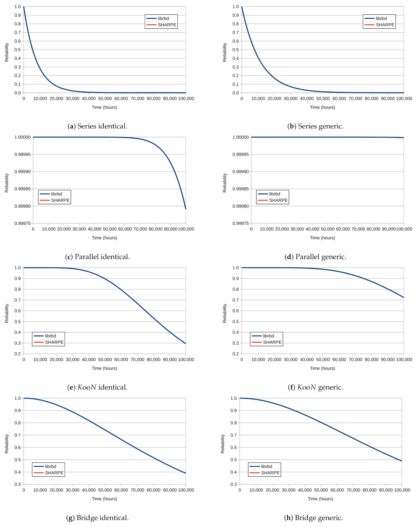
5.2. Comparison with SHARPE
6. Conclusions and Future Work
- Development of a tool that allows the graphical definition of RBDs and their analysis through the usage of librbd.
- Development of a tool that allows the graphical definition of hierarchical models (RBDs and STPNs/GSPNs) and that integrates librbd and SIRIO library for their quantitative evaluation.
- Usage of native Windows APIs for SMP to decrease the execution time on this OS.
- Investigation on the performance loss experienced for KooN block with generic components. This performance loss is visible with and it is probably due to a nonoptimized usage of the cache memory.
Author Contributions
Funding
Institutional Review Board Statement
Informed Consent Statement
Data Availability Statement
Conflicts of Interest
Abbreviations
| CTMC | Continuous Time Markov Chain |
| DFT | Dynamic FT |
| DRBD | Dynamic RBD |
| FT | Fault Tree |
| FTRE | FT with Repeated Events |
| GSPN | Generalized Stochastic Petri Net |
| OS | Operating System |
| RBD | Reliability Block Diagram |
| RG | Reliability Graph |
| SAN | Stochastic Activity Network |
| SMP | Symmetric Multi-Processing |
| SPN | Stochastic Petri Net |
| SRN | Stochastic Reward Net |
| STPN | Stochastic Time Petri Net |
References
- ISO/IEC/IEEE. International Standard-Systems and Software Engineering—Vocabulary; ISO/IEC/IEEE 24765:2010(E); IEEE: New York, NY, USA, 2010; pp. 1–418. [Google Scholar] [CrossRef]
- CENELEC. EN 50126-1: Railway Applications–The Specification and Demonstration of Reliability, Availability, Maintainability and Safety (RAMS)-Part 1: Generic RAMS Process; Technical Report; CENELEC: Brussels, Belgium, 2017. [Google Scholar]
- Trivedi, K.S.; Bobbio, A. Reliability and Availability Engineering; Cambridge University Press: Cambridge, UK, 2017. [Google Scholar] [CrossRef]
- Mahboob, Q.; Zio, E. Handbook of RAMS in Railway Systems: Theory and Practice; CRC Press: Boca Raton, FL, USA, 2018. [Google Scholar] [CrossRef]
- Moskowitz, F. The analysis of redundancy networks. Trans. Am. Inst. Electr. Eng. Part I Commun. Electron. 1958, 77, 627–632. [Google Scholar] [CrossRef]
- IEC. IEC 61078: Reliability Block Diagrams; Technical Report; IEC: Geneva, Switzerland, 2016. [Google Scholar]
- Hixenbaugh, A.F. Fault Tree for Safety; Technical Report; Boeing Aerospace Company: Seattle, WA, USA, 1968. [Google Scholar]
- IEC. IEC 61025: Fault Tree Analysis (FTA); Technical Report; IEC: Geneva, Switzerland, 2006. [Google Scholar]
- Rubino, G. Network reliability evaluation. In State-of-the-Art in Performance Modeling and Simulation; Gordon & Breach Books: London, UK, 1998. [Google Scholar]
- Bryant, R.E. Graph-Based Algorithms for Boolean Function Manipulation. IEEE Trans. Comput. 1986, C-35, 677–691. [Google Scholar] [CrossRef] [Green Version]
- Ericson, C. Fault Tree Analysis-A History. In Proceedings of the 17th International System Safety Conference, Orlando, FL, USA, 16–21 August 1999; pp. 1–9. [Google Scholar]
- Stewart, W. Introduction to the Numerical Solution of Markov Chains; Princeton University Press: Princeton, NJ, USA, 1994. [Google Scholar]
- IEC. IEC 61165: Application of Markov Techniques; Technical Report; IEC: Geneva, Switzerland, 2006. [Google Scholar]
- Molloy, M. Performance Analysis Using Stochastic Petri Nets. IEEE Trans. Comput. 1982, 31, 913–917. [Google Scholar] [CrossRef]
- Marsan, M.A.; Conte, G. A class of generalized stochastic petri nets for the performance evaluation of multiprocessor systems. ACM Trans. Comput. Syst. 1983, 2, 93–122. [Google Scholar] [CrossRef]
- Vicario, E.; Sassoli, L.; Carnevali, L. Using stochastic state classes in quantitative evaluation of dense-time reactive systems. IEEE Trans. Softw. Eng. 2009, 35, 703–719. [Google Scholar] [CrossRef]
- IEC. IEC 62551: Analysis Techniques for Dependability—Petri Net Techniques; Technical Report; IEC: Geneva, Switzerland, 2012. [Google Scholar]
- Ciardo, G.; Blakemore, A.; Chimento, P.F.; Muppala, J.K.; Trivedi, K.S. Automated Generation and Analysis of Markov Reward Models Using Stochastic Reward Nets. In Linear Algebra, Markov Chains, and Queueing Models; Meyer, C.D., Plemmons, R.J., Eds.; Springer-Verlag: New York, NY, USA, 1993; pp. 145–191. [Google Scholar]
- Ciardo, G.; Trivedi, K.S. A decomposition approach for stochastic reward net models. Perform. Eval. 1993, 18, 37–59. [Google Scholar] [CrossRef]
- Meyer, J.; Movaghar, A.; Sanders, W. Stochastic Activity Networks: Structure, Behavior, and Application. In Proceedings of the International Workshop on Timed Petri Nets, Torino, Italy, 1–3 July 1985; pp. 106–115. [Google Scholar]
- Sanders, W.H.; Meyer, J.F. Stochastic Activity Networks: Formal Definitions and Concepts. In Lectures on Formal Methods and Performance Analysis: First EEF/Euro Summer School on Trends in Computer Science Bergen Dal, The Netherlands, 3–7 July 2000; Hermanns, H., Katoen, J.-P., Brinksma, E., Eds.; Springer: Berlin/Heidelberg, Germany, 2000; pp. 315–343. [Google Scholar] [CrossRef]
- Malhotra, M.; Trivedi, K.S. Power-hierarchy of dependability-model types. IEEE Trans. Reliab. 1994, 43, 493–502. [Google Scholar] [CrossRef] [Green Version]
- Distefano, S.; Puliafito, A. Dynamic reliability block diagrams: Overview of a methodology. In Proceedings of the European Safety and Reliability Conference 2007, ESREL 2007-Risk, Reliability and Societal Safety, Stavanger, Norway, 25–27 June 2007; Volume 2. [Google Scholar]
- Distefano, S.; Puliafito, A. Dependability Evaluation with Dynamic Reliability Block Diagrams and Dynamic Fault Trees. IEEE Trans. Dependable Secur. Comput. 2009, 6, 4–17. [Google Scholar] [CrossRef]
- Dugan, J.B.; Bavuso, S.J.; Boyd, M.A. Dynamic fault-tree models for fault-tolerant computer systems. IEEE Trans. Reliab. 1992, 41, 363–377. [Google Scholar] [CrossRef] [Green Version]
- Codetta-Raiteri, D. The Conversion of Dynamic Fault Trees to Stochastic Petri Nets, as a case of Graph Transformation. Electron. Notes Theor. Comput. Sci. 2005, 127, 45–60. [Google Scholar] [CrossRef] [Green Version]
- Volk, M.; Weik, N.; Katoen, J.P.; Nießen, N. A DFT Modeling Approach for Infrastructure Reliability Analysis of Railway Station Areas. In Formal Methods for Industrial Critical Systems; Larsen, K.G., Willemse, T., Eds.; Springer International Publishing: Cham, Switzerland, 2019; pp. 40–58. [Google Scholar]
- Carnevali, L.; Ciani, L.; Fantechi, A.; Papini, M. A novel layered approach to evaluate reliability of complex systems. In Proceedings of the 2019 IEEE 5th International forum on Research and Technology for Society and Industry (RTSI), Florence, Italy, 9–12 September 2019; pp. 291–295. [Google Scholar] [CrossRef]
- Papini, M. Reliability Evaluation of an Industrial System Through Predictive Diagnostics. Ph.D. Thesis, Universitá degli Studi di Firenze, Florence, Italy, 2021. [Google Scholar]
- Iannino, A.; Musa, J.D. Software Reliability. In Advances in Computers; Marshall, C.Y., Ed.; Elsevier: Amsterdam, The Netherlands, 1990; Volume 30, pp. 85–170. [Google Scholar] [CrossRef]
- Lyu, M. Handbook of Software Reliability Engineering; McGraw-Hill, Inc.: New York, NY, USA, 1996. [Google Scholar]
- Mzyk, R.; Paszkiel, S. Influence of Program Architecture on Software Quality Attributes. In Control, Computer Engineering and Neuroscience; Paszkiel, S., Ed.; Springer International Publishing: Cham, Switzerland, 2021; pp. 322–329. [Google Scholar] [CrossRef]
- Wood, A. Predicting software reliability. Computer 1996, 29, 69–77. [Google Scholar] [CrossRef]
- Pham, H. System Software Reliability (Springer Series in Reliability Engineering); Springer-Verlag: Berlin/Heidelberg, Germany, 2006. [Google Scholar] [CrossRef]
- Ballerini, S.; Carnevali, L.; Paolieri, M.; Tadano, K.; Machida, F. Software rejuvenation impacts on a phased-mission system for Mars exploration. In Proceedings of the 2013 IEEE International Symposium on Software Reliability Engineering Workshops (ISSREW), Pasadena, CA, USA, 4–7 November 2013; pp. 275–280. [Google Scholar] [CrossRef]
- Paolieri, M.; Biagi, M.; Carnevali, L.; Vicario, E. The ORIS Tool: Quantitative Evaluation of Non-Markovian Systems. IEEE Trans. Softw. Eng. 2019, in press. [Google Scholar] [CrossRef]
- RBDTool. Web Page. Available online: http://pages.mtu.edu/~pjbonamy/rbdtool.html (accessed on 13 November 2019).
- Edraw Block Diagram. Web Page. Available online: https://www.edrawsoft.com/reliability-block-diagram-software.php (accessed on 23 April 2021).
- Reliability Workbench. Web Page. Available online: https://www.isograph.com/software/reliability-workbench/rbd-analysis/ (accessed on 23 April 2021).
- Relyence RBD. Web Page. Available online: https://www.relyence.com/products/rbd/ (accessed on 23 April 2021).
- Sahner, R.A.; Trivedi, K.S.; Puliafito, A. Performance and Reliability Analysis of Computer Systems: An Example-Based Approach Using the SHARPE Software Package; Kluwer Academic Publishers: Alphen aan den Rijn, The Netherlands, 1996. [Google Scholar] [CrossRef]
- SHARPE. Web Page. Available online: https://sharpe.pratt.duke.edu/ (accessed on 23 April 2021).
- librbd. Web Page. Available online: https://github.com/marcopapini/librbd (accessed on 23 April 2021).
- Siewiorek, D.P.; Swarz, R.S. Reliable Computer Systems: Design and Evaluation, 3rd ed.; A. K. Peters, Ltd.: Natick, MA, USA, 1998. [Google Scholar]
- Catelani, M.; Ciani, L.; Venzi, M. RBD Model-Based Approach for Reliability Assessment in Complex Systems. IEEE Syst. J. 2019, 13, 2089–2097. [Google Scholar] [CrossRef]
- Fourment, M.; Gillings, M. A comparison of common programming languages used in bioinformatics. BMC Bioinform. 2008, 9, 82. [Google Scholar] [CrossRef] [PubMed] [Green Version]
- IEEE. IEEE. IEEE Standard for Floating-Point Arithmetic. In IEEE Std-754-2019 (Revision IEEE-754-2008); IEEE: New York, NY, USA, 2019; pp. 1–84. [Google Scholar] [CrossRef]
- IEEE. IEEE. IEEE Standard for Information Technology–Portable Operating System Interface (POSIX™) Base Specifications, Issue 7. In IEEE Std 1003.1-2017 (Revision of IEEE Std 1003.1-2008); IEEE: New York, NY, USA, 2018; pp. 1–3951. [Google Scholar] [CrossRef]
- pthreads-win32. Web Page. Available online: http://sourceware.org/pthreads-win32/ (accessed on 23 April 2021).
- Cygwin. Web Page. Available online: https://www.cygwin.com/ (accessed on 23 April 2021).
- Telcordia SR-332. Reliability Prediction Procedure for Electronic Equipment; Technical Report Issue 4; Telcordia Network Infrastructure Solutions (NIS): Bridgewater, NJ, USA, 2016. [Google Scholar]


| Component | Failure Rate ( | Component | Failure Rate ( |
|---|---|---|---|
| C1 | 0.0000084019 | C9 | 0.0000027777 |
| C2 | 0.0000039438 | C10 | 0.0000055397 |
| C3 | 0.0000078310 | C11 | 0.0000047740 |
| C4 | 0.0000079844 | C12 | 0.0000062887 |
| C5 | 0.0000091165 | C13 | 0.0000036478 |
| C6 | 0.0000019755 | C14 | 0.0000051340 |
| C7 | 0.0000033522 | C15 | 0.0000095223 |
| C8 | 0.0000076823 | ||
| RBD Block | Topology | T (h) | Components |
|---|---|---|---|
| Series identical | 15 components | C1 | |
| Series generic | 15 components | All | |
| Parallel identical | 15 components | C1 | |
| Parallel generic | 15 components | All | |
| KooN identical | 8oo15 | C1 | |
| KooN generic | 8oo15 | All | |
| Bridge identical | 5 components | C1 | |
| Bridge generic | 5 components | From C1 to C5 |
| RBD Block | Error Function | |
|---|---|---|
| Minimum | Maximum | |
| Series identical | −1.00 × | 1.00 × |
| Series generic | −1.00 × | 1.00 × |
| Parallel identical | 0.00 × | 0.00 × |
| Parallel generic | 0.00 × | 0.00 × |
| KooN identical | −1.00 × | 0.00 × |
| KooN generic | −1.00 × | 0.00 × |
| Bridge identical | 0.00 × | 0.00 × |
| Bridge generic | 0.00 × | 0.00 × |
| Name | Chassis | CPU & RAM | OS & Compiler |
|---|---|---|---|
| PC1 | Workstation | Intel i7-2600 | Ubuntu |
| @ GHz | _amd64 | ||
| 16GB-DDR3 | GCC | ||
| @ 1333MHz | |||
| PC2 | Notebook | Intel i7-6700HQ | Mac OS |
| @ GHz | |||
| 16GB-LPDDR3 | Apple LLVM | ||
| @ 2133MHz | |||
| PC3 | Notebook | Intel i7-7700HQ | Ubuntu |
| @ GHz | _amd64 | ||
| 32GB-DDR4 | GCC | ||
| @ 2400MHz | |||
| PC4 | Notebook | Intel i5-8365U | Windows |
| @ GHz | 10 | ||
| 16GB-DDR4 | Cygwin GCC | ||
| @ 2666MHz | |||
| PC5 | Raspberry Pi 3 | Raspberry Pi OS | |
| @ GHz | 10_AArch32 | ||
| 1GB-LPDDR2 | GCC | ||
| @ 900MHz |
| Topology | # Times | Execution Time (ms) | ||||
|---|---|---|---|---|---|---|
| PC1 | PC2 | PC3 | PC4 | PC5 | ||
| 2 | 50,000 | 0.436 | 0.268 | 0.228 | 0.657 | 2.812 |
| 2 | 100,000 | 0.247 | 0.365 | 0.290 | 0.896 | 4.336 |
| 2 | 200,000 | 0.548 | 0.706 | 0.621 | 1.692 | 8.156 |
| 3 | 50,000 | 0.174 | 0.260 | 0.228 | 0.671 | 2.446 |
| 3 | 100,000 | 0.380 | 0.419 | 0.307 | 0.904 | 4.732 |
| 3 | 200,000 | 0.701 | 0.851 | 0.657 | 1.659 | 11.720 |
| 5 | 50,000 | 0.193 | 0.264 | 0.289 | 0.646 | 4.229 |
| 5 | 100,000 | 0.412 | 0.394 | 0.436 | 0.927 | 6.505 |
| 5 | 200,000 | 0.902 | 0.792 | 0.729 | 1.767 | 13.761 |
| 10 | 50,000 | 0.351 | 0.351 | 0.317 | 0.706 | 8.312 |
| 10 | 100,000 | 0.884 | 0.637 | 0.634 | 1.021 | 13.734 |
| 10 | 200,000 | 1.754 | 1.190 | 1.144 | 1.972 | 27.330 |
| 15 | 50,000 | 0.538 | 0.491 | 0.433 | 0.760 | 11.697 |
| 15 | 100,000 | 1.279 | 0.873 | 0.848 | 1.117 | 20.715 |
| 15 | 200,000 | 2.650 | 1.831 | 1.646 | 2.034 | 41.191 |
| Topology | # Times | Execution Time (ms) | ||||
|---|---|---|---|---|---|---|
| PC1 | PC2 | PC3 | PC4 | PC5 | ||
| 2 | 50,000 | 0.388 | 0.263 | 0.220 | 0.633 | 2.325 |
| 2 | 100,000 | 0.252 | 0.343 | 0.290 | 0.958 | 3.785 |
| 2 | 200,000 | 0.511 | 0.638 | 0.597 | 1.709 | 6.790 |
| 3 | 50,000 | 0.163 | 0.255 | 0.205 | 0.690 | 1.510 |
| 3 | 100,000 | 0.365 | 0.370 | 0.306 | 0.869 | 3.521 |
| 3 | 200,000 | 0.602 | 0.774 | 0.626 | 1.558 | 6.591 |
| 5 | 50,000 | 0.179 | 0.260 | 0.253 | 0.683 | 1.865 |
| 5 | 100,000 | 0.329 | 0.356 | 0.411 | 0.856 | 3.098 |
| 5 | 200,000 | 0.561 | 0.690 | 0.694 | 1.740 | 6.862 |
| 10 | 50,000 | 0.287 | 0.267 | 0.274 | 0.667 | 2.146 |
| 10 | 100,000 | 0.532 | 0.379 | 0.438 | 0.925 | 4.041 |
| 10 | 200,000 | 0.673 | 0.725 | 0.737 | 1.839 | 8.507 |
| 15 | 50,000 | 0.413 | 0.314 | 0.347 | 0.737 | 2.419 |
| 15 | 100,000 | 0.573 | 0.469 | 0.565 | 0.932 | 4.262 |
| 15 | 200,000 | 0.874 | 0.933 | 0.935 | 1.874 | 7.831 |
| Topology | # Times | Execution Time (ms) | ||||
|---|---|---|---|---|---|---|
| PC1 | PC2 | PC3 | PC4 | PC5 | ||
| 2 | 50,000 | 0.197 | 0.310 | 0.204 | 0.685 | 1.978 |
| 2 | 100,000 | 0.278 | 0.430 | 0.392 | 0.858 | 4.053 |
| 2 | 200,000 | 0.594 | 0.861 | 0.635 | 1.588 | 8.407 |
| 3 | 50,000 | 0.183 | 0.295 | 0.198 | 0.655 | 3.190 |
| 3 | 100,000 | 0.356 | 0.432 | 0.456 | 0.884 | 5.626 |
| 3 | 200,000 | 0.691 | 0.804 | 0.663 | 1.698 | 11.161 |
| 5 | 50,000 | 0.206 | 0.313 | 0.226 | 0.686 | 4.056 |
| 5 | 100,000 | 0.474 | 0.433 | 0.456 | 0.951 | 7.139 |
| 5 | 200,000 | 0.940 | 0.858 | 0.734 | 1.655 | 14.948 |
| 10 | 50,000 | 0.446 | 0.355 | 0.419 | 0.651 | 9.915 |
| 10 | 100,000 | 0.879 | 0.617 | 0.709 | 0.947 | 16.667 |
| 10 | 200,000 | 1.797 | 1.232 | 1.110 | 1.891 | 29.725 |
| 15 | 50,000 | 0.548 | 0.440 | 0.552 | 0.765 | 13.544 |
| 15 | 100,000 | 1.347 | 0.945 | 0.896 | 1.089 | 22.388 |
| 15 | 200,000 | 2.649 | 1.853 | 1.916 | 2.110 | 42.094 |
| Topology | # Times | Execution Time (ms) | ||||
|---|---|---|---|---|---|---|
| PC1 | PC2 | PC3 | PC4 | PC5 | ||
| 2 | 50,000 | 0.181 | 0.302 | 0.199 | 0.641 | 1.406 |
| 2 | 100,000 | 0.260 | 0.396 | 0.342 | 0.838 | 3.983 |
| 2 | 200,000 | 0.523 | 0.821 | 0.629 | 1.627 | 7.381 |
| 3 | 50,000 | 0.178 | 0.292 | 0.197 | 0.642 | 1.637 |
| 3 | 100,000 | 0.360 | 0.423 | 0.444 | 0.831 | 3.316 |
| 3 | 200,000 | 0.566 | 0.756 | 0.623 | 1.630 | 6.872 |
| 5 | 50,000 | 0.187 | 0.292 | 0.224 | 0.704 | 2.093 |
| 5 | 100,000 | 0.401 | 0.383 | 0.438 | 0.868 | 3.784 |
| 5 | 200,000 | 0.594 | 0.776 | 0.673 | 1.527 | 7.597 |
| 10 | 50,000 | 0.290 | 0.284 | 0.315 | 0.627 | 2.068 |
| 10 | 100,000 | 0.561 | 0.394 | 0.489 | 0.854 | 4.145 |
| 10 | 200,000 | 0.718 | 0.754 | 0.718 | 1.700 | 7.429 |
| 15 | 50,000 | 0.388 | 0.305 | 0.347 | 0.688 | 2.522 |
| 15 | 100,000 | 0.642 | 0.476 | 0.552 | 0.918 | 4.626 |
| 15 | 200,000 | 0.801 | 0.892 | 0.951 | 1.997 | 8.311 |
| Topology | # Times | Execution Time (ms) | ||||
|---|---|---|---|---|---|---|
| PC1 | PC2 | PC3 | PC4 | PC5 | ||
| 1oo2 | 50,000 | 0.183 | 0.306 | 0.211 | 0.667 | 1.810 |
| 1oo2 | 100,000 | 0.254 | 0.402 | 0.393 | 0.791 | 3.873 |
| 1oo2 | 200,000 | 0.561 | 0.782 | 0.617 | 1.540 | 8.123 |
| 2oo3 | 50,000 | 0.669 | 0.768 | 0.709 | 0.776 | 6.478 |
| 2oo3 | 100,000 | 1.265 | 1.278 | 1.280 | 1.163 | 12.146 |
| 2oo3 | 200,000 | 2.724 | 2.299 | 2.787 | 2.122 | 21.686 |
| 3oo5 | 50,000 | 2.453 | 2.419 | 2.716 | 2.103 | 30.528 |
| 3oo5 | 100,000 | 4.313 | 5.402 | 4.468 | 4.090 | 44.617 |
| 3oo5 | 200,000 | 7.224 | 9.466 | 8.448 | 7.611 | 82.247 |
| 5oo10 | 50,000 | 20.584 | 45.096 | 20.462 | 35.188 | 299.916 |
| 5oo10 | 100,000 | 44.083 | 88.876 | 46.227 | 78.124 | 506.973 |
| 5oo10 | 200,000 | 78.657 | 178.793 | 80.726 | 288.728 | 986.001 |
| 8oo15 | 50,000 | 558.292 | 1212.422 | 571.278 | 1838.166 | 7753.987 |
| 8oo15 | 100,000 | 1167.856 | 2406.377 | 1194.093 | 3694.708 | 15,316.800 |
| 8oo15 | 200,000 | 2233.662 | 4784.158 | 2278.303 | 7666.604 | 30,172.290 |
| Topology | # Times | Execution Time (ms) | ||||
|---|---|---|---|---|---|---|
| PC1 | PC2 | PC3 | PC4 | PC5 | ||
| 1oo2 | 50,000 | 0.171 | 0.293 | 0.199 | 0.617 | 1.397 |
| 1oo2 | 100,000 | 0.250 | 0.378 | 0.367 | 0.805 | 3.613 |
| 1oo2 | 200,000 | 0.533 | 0.748 | 0.598 | 1.537 | 8.085 |
| 2oo3 | 50,000 | 0.377 | 0.334 | 0.380 | 0.649 | 3.745 |
| 2oo3 | 100,000 | 0.616 | 0.482 | 0.718 | 1.002 | 6.674 |
| 2oo3 | 200,000 | 0.980 | 0.856 | 1.149 | 2.099 | 12.279 |
| 3oo5 | 50,000 | 0.491 | 0.372 | 0.579 | 0.964 | 5.452 |
| 3oo5 | 100,000 | 0.840 | 0.682 | 0.882 | 1.148 | 9.192 |
| 3oo5 | 200,000 | 1.251 | 1.244 | 1.513 | 2.056 | 15.876 |
| 5oo10 | 50,000 | 0.658 | 0.708 | 0.764 | 0.961 | 10.244 |
| 5oo10 | 100,000 | 1.315 | 1.396 | 1.220 | 1.309 | 15.746 |
| 5oo10 | 200,000 | 2.169 | 2.339 | 1.990 | 4.621 | 28.266 |
| 8oo15 | 50,000 | 1.422 | 1.168 | 1.720 | 2.651 | 18.303 |
| 8oo15 | 100,000 | 3.027 | 2.456 | 2.810 | 4.756 | 27.901 |
| 8oo15 | 200,000 | 4.403 | 4.035 | 4.940 | 10.613 | 48.033 |
| Topology | # Times | Execution Time (ms) | ||||
|---|---|---|---|---|---|---|
| PC1 | PC2 | PC3 | PC4 | PC5 | ||
| 1oo15 | 100,000 | 1.280 | 0.765 | 0.929 | 2.305 | 17.021 |
| 2oo15 | 100,000 | 10.944 | 10.057 | 9.167 | 24.552 | 88.657 |
| 3oo15 | 100,000 | 73.165 | 61.577 | 64.344 | 155.191 | 571.809 |
| 4oo15 | 100,000 | 183.721 | 341.797 | 183.270 | 604.827 | 2025.680 |
| 5oo15 | 100,000 | 406.931 | 836.953 | 418.733 | 1297.444 | 4983.553 |
| 6oo15 | 100,000 | 740.532 | 1503.090 | 753.573 | 2314.167 | 9237.214 |
| 7oo15 | 100,000 | 1062.330 | 2126.853 | 1071.369 | 3260.557 | 13,325.713 |
| 8oo15 | 100,000 | 1190.309 | 2386.732 | 1192.385 | 4171.043 | 15,280.717 |
| 9oo15 | 100,000 | 1064.583 | 2134.690 | 1052.093 | 3688.210 | 13,398.969 |
| 10oo15 | 100,000 | 742.056 | 1511.135 | 758.824 | 2466.044 | 9164.543 |
| 11oo15 | 100,000 | 411.900 | 837.570 | 417.853 | 1287.806 | 4967.779 |
| 12oo15 | 100,000 | 183.203 | 341.557 | 189.317 | 590.764 | 2015.668 |
| 13oo15 | 100,000 | 62.120 | 107.026 | 72.951 | 107.102 | 664.601 |
| 14oo15 | 100,000 | 9.432 | 15.416 | 10.368 | 17.220 | 100.526 |
| 15oo15 | 100,000 | 1.440 | 0.933 | 1.041 | 2.163 | 18.609 |
| Topology | # Times | Execution Time (ms) | ||||
|---|---|---|---|---|---|---|
| PC1 | PC2 | PC3 | PC4 | PC5 | ||
| 1oo15 | 100,000 | 0.663 | 0.430 | 0.635 | 2.083 | 4.653 |
| 2oo15 | 100,000 | 0.828 | 0.883 | 0.884 | 2.908 | 8.284 |
| 3oo15 | 100,000 | 1.154 | 1.185 | 1.064 | 3.054 | 11.596 |
| 4oo15 | 100,000 | 1.454 | 1.401 | 1.402 | 3.385 | 14.935 |
| 5oo15 | 100,000 | 1.848 | 1.660 | 1.535 | 3.183 | 18.000 |
| 6oo15 | 100,000 | 2.147 | 1.898 | 1.723 | 3.513 | 21.169 |
| 7oo15 | 100,000 | 2.478 | 2.136 | 1.968 | 3.734 | 24.497 |
| 8oo15 | 100,000 | 3.063 | 2.475 | 2.831 | 5.842 | 27.787 |
| 9oo15 | 100,000 | 2.731 | 2.118 | 2.596 | 6.283 | 24.446 |
| 10oo15 | 100,000 | 2.432 | 1.900 | 2.418 | 4.917 | 21.156 |
| 11oo15 | 100,000 | 2.072 | 1.646 | 1.931 | 3.696 | 18.043 |
| 12oo15 | 100,000 | 1.562 | 1.414 | 1.666 | 3.144 | 14.822 |
| 13oo15 | 100,000 | 1.240 | 1.181 | 1.340 | 2.564 | 11.546 |
| 14oo15 | 100,000 | 0.933 | 0.935 | 1.128 | 2.342 | 8.221 |
| 15oo15 | 100,000 | 0.635 | 0.464 | 0.641 | 1.980 | 4.719 |
| # Times | Execution Time (ms) | ||||
|---|---|---|---|---|---|
| PC1 | PC2 | PC3 | PC4 | PC5 | |
| 50,000 | 0.253 | 0.263 | 0.240 | 1.361 | 2.962 |
| 100,000 | 0.406 | 0.449 | 0.452 | 1.736 | 5.967 |
| 200,000 | 0.853 | 0.823 | 0.774 | 3.375 | 10.985 |
| # Times | Execution Time (ms) | ||||
|---|---|---|---|---|---|
| PC1 | PC2 | PC3 | PC4 | PC5 | |
| 50,000 | 0.235 | 0.248 | 0.218 | 1.377 | 1.600 |
| 100,000 | 0.338 | 0.341 | 0.395 | 1.673 | 3.272 |
| 200,000 | 0.548 | 0.706 | 0.649 | 3.293 | 7.289 |
| RBD Block | Topology | Execution Time (s) | Gain (%) | |
|---|---|---|---|---|
| librbd | SHARPE | |||
| Series generic | 2 | 0.10 | 0.98 | 89.95 |
| 3 | 0.10 | 1.12 | 91.04 | |
| 5 | 0.11 | 0.98 | 88.97 | |
| 10 | 0.10 | 1.94 | 94.60 | |
| 15 | 0.10 | 2.59 | 96.19 | |
| Series identical | 2 | 0.10 | 0.90 | 89.24 |
| 3 | 0.11 | 0.96 | 88.32 | |
| 5 | 0.11 | 0.90 | 87.72 | |
| 10 | 0.12 | 1.23 | 90.40 | |
| 15 | 0.10 | 1.45 | 93.31 | |
| Parallel generic | 2 | 0.11 | 0.98 | 89.08 |
| 3 | 0.10 | 1.12 | 91.20 | |
| 5 | 0.11 | 0.98 | 89.22 | |
| 10 | 0.10 | 2.03 | 94.95 | |
| 15 | 0.10 | 2.78 | 96.36 | |
| Parallel identical | 2 | 0.10 | 0.92 | 89.19 |
| 3 | 0.11 | 0.95 | 88.74 | |
| 5 | 0.11 | 0.92 | 88.51 | |
| 10 | 0.12 | 1.31 | 91.16 | |
| 15 | 0.10 | 1.59 | 93.85 | |
| KooN generic | 1oo2 | 0.11 | 1.01 | 89.37 |
| 2oo3 | 0.12 | 1.15 | 89.95 | |
| 3oo5 | 0.11 | 1.01 | 89.44 | |
| 5oo10 | 0.15 | 2.28 | 93.21 | |
| 8oo15 | 2.35 | 3.36 | 29.96 | |
| KooN identical | 1oo2 | 0.11 | 0.88 | 87.80 |
| 2oo3 | 0.11 | 0.89 | 88.13 | |
| 3oo5 | 0.11 | 0.88 | 87.71 | |
| 5oo10 | 0.08 | 1.31 | 94.20 | |
| 8oo15 | 0.08 | 1.81 | 95.71 | |
| Bridge generic | 5 | 0.10 | 1.64 | 94.16 |
| Bridge identical | 5 | 0.09 | 1.66 | 94.35 |
Publisher’s Note: MDPI stays neutral with regard to jurisdictional claims in published maps and institutional affiliations. |
© 2021 by the authors. Licensee MDPI, Basel, Switzerland. This article is an open access article distributed under the terms and conditions of the Creative Commons Attribution (CC BY) license (https://creativecommons.org/licenses/by/4.0/).
Share and Cite
Carnevali, L.; Ciani, L.; Fantechi, A.; Gori, G.; Papini, M. An Efficient Library for Reliability Block Diagram Evaluation. Appl. Sci. 2021, 11, 4026. https://doi.org/10.3390/app11094026
Carnevali L, Ciani L, Fantechi A, Gori G, Papini M. An Efficient Library for Reliability Block Diagram Evaluation. Applied Sciences. 2021; 11(9):4026. https://doi.org/10.3390/app11094026
Chicago/Turabian StyleCarnevali, Laura, Lorenzo Ciani, Alessandro Fantechi, Gloria Gori, and Marco Papini. 2021. "An Efficient Library for Reliability Block Diagram Evaluation" Applied Sciences 11, no. 9: 4026. https://doi.org/10.3390/app11094026