Abstract
Radio-frequency spectrum resources are finite and scarce, but their demand is increasing exponentially every year. Therefore, wireless network resources are too expensive to be wasted. To avoid waste, pricing techniques can efficiently control resource usage and manage user needs in networks. This study focuses on QoS-aware pricing for usage-based mobile Internet access charging. Specifically, I propose a heuristic algorithm for priority pricing with multiple service levels. The proposed algorithm is built on top of the existing equilibrium analysis methods. While being extensively studied for optimal price selection, the equilibrium methods make a few unrealistic assumptions, and so my methods adjust the solutions of the equilibrium methods to account for distortions that the real world creates. The evaluation results indicate that multiple equilibrium prices may exist, and the proposed scheme produces a pricing plan that is substantially more effective than existing equilibrium methods.
1. Introduction
Radio-frequency spectrum resources are finite and scarce, but their demand is increasing exponentially every year [1]. Although today’s fast wireless communication technologies enable us to enjoy various newly-devised services, these services are causing more congestion in wireless networks. To resolve this problem, studies have been conducted on the efficient use of wireless resources [2]. Pricing is one of the techniques used to effectively control network resource usage and manage user demands [3].
Pricing network services has been an issue of continuous debate since the early stages of Internet commercialization. Historically, the flat-fee scheme in which users are charged a fixed monthly fee irrespective of usage has been the predominant pricing structure for wired Internet access services, as both service providers and consumers prefer simple pricing to usage-sensitive pricing [1,4].
However, pricing schemes other than the flat-fee scheme have begun to emerge in some domains, such as with wireless Internet access. In wireless networks, the bandwidth is too scarce and expensive to tolerate the potential waste of resources, which is typically associated with flat-fee pricing [5]. The evolution of mobile devices (e.g., smartphones and IoT devices) has caused traffic to explode, and the congestion of wireless networks is becoming more serious, jeopardizing the provision of stable quality of service (QoS). Wireless carriers have already dropped their unlimited flat-fee policy, and currently offer various pricing policies that combine fixed charging up to a certain data cap, and usage-based charging beyond that cap.
Internet applications have different levels of QoS requirements, such as delay, latency, and goodput. The coexistence of applications with high QoS (such as automatic driving or VR interaction) with those with low QoS (such as emails) requires wireless networks to handle the corresponding traffic differently. The IETF differentiated service [6,7,8] is the currently preferred Internet QoS architecture. Traffic is differentiated based on the traffic class information in the IP packet headers and is served according to some form of priority-based scheduling. The architecture of current mobile network QoS is more complicated. According to the characteristics of user equipment (UE) and its services, various priority classes are necessary in the mobile network. For example, 5G mobile networks specify three service types: guaranteed bit rate (GBR) service, non-GBR service, and delay-critical GBR service, along with QoS classes defined by resource type, priority level, packet delay budget, packet error rate, maximum data burst volume, and averaging window [9]. Currently, many wireless providers have announced their plans to implement a priority pricing policy (i.e., different pricing for different traffic classes). The single-price scheme is the simplest form of priority pricing.
In usage-based charging, a certain price is charged for a certain amount of data (e.g., Mbytes). Under usage-based charging, either the single-price scheme or priority-pricing scheme, determining the price(s) is a crucial issue. This study focuses on optimal price selection for “priority pricing” [3,10,11]; that is, finding the prices that maximize a certain system objective. Other pricing schemes have been studied: smart-market pricing [12,13], Paris-metro pricing [14,15], responsive pricing [16], edge pricing [17,18], proportional fairness pricing [19], and distributed majorization pricing [20]. Along with priority pricing, all of these schemes assume that the users are inherently price-sensitive and that the service provider can use prices to influence the behaviors of the users as a means of congestion control.
Under priority pricing, the service provider offers a choice of {service level, price} pairs, and the users, who know the values of their jobs, select the service levels that they would like to use. A user chooses the service level depending on the QoS requirements as well as the service price. For example, if a service level becomes bad, some users may decide to pay more and use a higher-level service, and vice versa. If there is no level whose service is worth the price, the user may decide not to send any traffic. The dynamics of a priority pricing system have often been modeled using equilibrium analysis [11,21,22,23,24,25,26,27,28].
The proposed scheme is built on top of the existing equilibrium analysis methods. The scheme adjusts the results of the equilibrium methods to account for the distortions created by realistic mobile internet access environments. The existing equilibrium analysis methods commonly assume that: (a) the individual user’s impact on the system is infinitesimal, and (b) users have up-to-date global knowledge of the system status, such as the queue length or the job arrival rate at each service level, which is crucial if users are to make optimal decisions [29]. However, when a finite (potentially small) number of users makes suboptimal decisions, as a result of inaccurate knowledge of the system status, a stable equilibrium may not always exist. Such a scenario is very possible in the case of wireless Internet access, as the number of users attached to a base station is typically small, and up-to-date knowledge of the system status is not available to the users.
The impact of using outdated information to determine network service pricing has been addressed in [11,30]. However, these studies deal with dynamic pricing, in which the service provider dynamically updates prices at run time. My scheme considers a static pricing system in which the prices do not change at run time, which is much more practical than dynamic pricing. This work differs from the equilibrium analysis of unobservable queues [27,28,31,32,33], in that it models explicit queues that are observable but have a delay in feeding the queue information to users.
My analysis indicates that the system often fails to converge to a stationary equilibrium in realistic environments. As a result, equilibrium methods may produce suboptimal prices. The suggested scheme effectively adjusts the suboptimal price selection of the equilibrium methods when the system does not converge to a stationary equilibrium. It uses a heuristic search algorithm with pruning built on a sliding window transition model. Note that Cao et al. [11] showed the existence of multiple equilibrium delays, whereas this work deals with equilibrium prices.
The remainder of this paper is organized as follows: Section 2 describes the general system framework used in this study. Section 3 describes the model of system behavior. Section 4 describes the analysis of the results of the existing equilibrium method using the model presented in Section 3. Section 5 describes how to adjust the results of the equilibrium method. Finally, Section 6 concludes the paper by presenting an overview of the paper and suggesting a future research.
2. System Framework
This study considers the price selection problem over a single-hop network link. The network offers different service levels to the users. Without loss of generality, let us call the highest priority level 1 and the lowest priority level I. For service level i, the service provider charges per data unit. The service provider determines the price vector of I service levels, , with a certain objective, such as maximizing system profit or net value of the system. I assume that prices do not change once this vector is determined. However, multiple pricing policies can be implemented according to the various user and traffic scenarios using the suggested scheme, and wireless service providers may change the price policy accordingly.
Let us call each user request to be transmitted a ‘job.’ The jobs are basically packets with QoS information. A user should negotiate with a base station to submit a job. He/She may decide not to submit the job if the cost is too expensive. When submitting a job, each user would essentially be requesting that the job be processed for the transmission. The submitted jobs are distributed to the priority queues by a classifier according to their types categorized by their QoS requirements. Here, the framework assumes that there are j types of QoS requirements, and each job is associated with QoS type j. The scheduler chooses a job from the front of a non-empty priority queue according to its scheduling discipline and thrusts the chosen job into the sending queue. For example, a scheduler using a priority queuing (PQ) discipline serves the job with the highest priority first and uses all the bandwidths to send the jobs in the sending queue. By contrast, a scheduler using a weighted fair queuing (WFQ) discipline would allocate the bandwidths to each priority queue according to its weight [34]. Subsequently, the base station and the corresponding UE would prepare the radio resource to transmit the jobs. A scheduling model is shown in Figure 1.
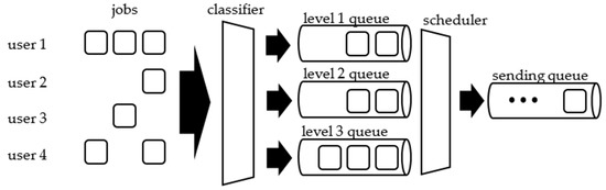
Figure 1.
PQ scheduling model.
Although each job has a different size, performance requirements, and error characteristics, I consider that a job’s completion delay is the main performance metric that determines its value. Thus, let us denote a job’s utility function by , where is the expected time to complete a type-j job when assigned to level i. It is natural to assume that is a non-increasing function with respect to .
The proposed framework considers a non-preemptive strict priority scheduling (SPS) discipline, although the basic concept of this study is not tied to a particular scheduling discipline. Because no guarantee can be made on the exact completion time under SPS, this framework uses the expected completion time. The computation of depends on many factors, such as the job arrival process, job service process, and job size. For example, under Poisson job arrival and exponential job length assumptions, with SPS can be computed using the M/M/1 priority queuing model, as shown in Equation (1):
where is the job service rate, is the job arrival rate for level k, is the average size of a type-j job, and is the average size of all jobs. The mathematical expression represents the job service time and represents the average waiting time of the job. Note that and are calculated from the empirical observations, although the job size has an exponential distribution. Readers may refer to [35] for the proof of Equation (1).
The expected job completion time is computed assuming that the queues associated with each service level are in a steady state. This assumption is appropriate for reasonably long broadcast intervals. Broadcast intervals are discussed in the last paragraph of this section, and update times longer than the time required to adjust to the new steady state are often sensible. The user may adopt a formula that considers transient states.
A user selects the service level of his jobs based solely on self-interest, and they are oblivious to the system objective. A user may decide not to submit a job, but he/she cannot change his/her decision once the job has been submitted. I assume that job arrival at each service level follows the Poisson process. The job arrival rate at service level i is denoted by , and is the job arrival rate vector. For notational convenience, denotes the arrival rate of jobs that were not submitted. When the total job arrival rate is , the sum of the job arrival rates at all levels is equal to (i.e., ). The network serves jobs at a rate of , which is essentially determined by the capacity of the wireless network. The capacity of a wireless network is often variable, as the wireless channel condition fluctuates, and the link throughput depends on the channel condition. In such cases, existing methods for estimating wireless link capacity may be used [36,37]. To achieve system stability, the effective job arrival rate must be smaller than .
I assume that the system status is periodically broadcast and that users make decisions based on the latest broadcast instead of the actual (but unknown) job arrival rates between the periodic updates. This assumption is reasonable for wireless networks, because all existing wireless access technologies use some form of periodic system broadcast channels (e.g., beacons). Keeping an accurate track of for each user by sniffing all of the network traffic is usually infeasible in wireless networks, and for each user to ask the network for the current whenever he has a job to send is undesirable for efficiency reasons.
Because this study assumes that each user’s decision is based solely on self-interest, a user with a type-j job is assumed to select the service level i that maximizes his utility value minus the associated cost, regardless of the system objective. The following expression captures the decision-making process of a user with a type-j job:
If the utility value minus the cost is negative for all levels, the user will not submit the job. The user’s decision depends on (in Equation (2)), and depends on the job arrival rates at higher levels (in Equation (1)). The job arrival rates, in turn, depend on the decisions of other users. This interdependency raises the possibility of system oscillation. Note that while pricing is static, the decisions made by users may be dynamic.
3. System Behavior Analysis Model
The suggested model, system behavior analysis model (SAM), is a state transition model that uses a price vector as an input and produces a system state transition graph by estimating the decisions of users. This graph, in which each state is identified by the associated job arrival rate vector , depicts the evolution of the system behavior over time. The state transition is discrete and occurs only when new values of are broadcast, as shown in Figure 2. St denotes the system state at time t, and denotes the job arrival rate vector at St. The transition of the system state is derived by modeling the decisions of individual users. Recall that users make decisions based on the knowledge that is currently available, , which remains fixed between updates. The actual may change as a result of the users’ decisions during the interval between broadcasts, but this new is not available for users to base their decisions on.
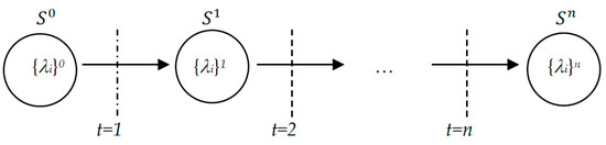
Figure 2.
Transition over time.
Depending on whether a given guarantees that the system converges on a steady state, SAM handles the two cases differently. When the system converges, the SAM produces a single of the convergent system state. On the other hand, when the system oscillates, the SAM computes a set of s. System divergence (i.e., oscillation among an infinite number of states) is theoretically possible but does not occur because the resolution of broadcast values is finite. The simulation indicates that this set contains a small number of states in most cases. Each in this set represents a recurring system state in the oscillation loop and is associated with a probability that indicates how long the system will stay in that corresponding state.
The SAM first estimates the most preferred service level for each job type in a certain system state. For all pairs of (i, j), it computes the Bernoulli variable, , which takes ‘1′ if the level i is the most profitable choice for a type-j job for the given price vector when the system is at St and takes ‘0’ otherwise. That is,
where is the expected completion time of a type-j job at level i at state . Note that the user’s decision between time t and t + 1 is based on .
Second, using , the SAM computes the probability that level i is selected at , by the following equation:
where is the probability that a job is of type j.
Finally, using , the SAM computes the job arrival rate vector at , , as follows:
In this way, the SAM constructs a state transition graph where a node corresponds to a system state visited, and a directional arc indicates a transition from one system state to another. The transition of may end up as a single state, as shown in Figure 3a, or may oscillate, as shown in Figure 3b. In the latter case, the stationary probability at each state S, W(S), in the oscillation loop is computed by counting the visit frequency.
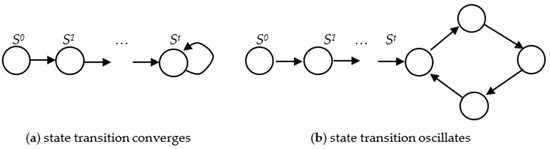
Figure 3.
Examples of a state transition graph.
So far, when computing , only the jobs that have arrived over one broadcast interval between (t−1) and t are considered. I implicitly assumed that the size of the broadcast interval was equal to that of the interval over which the job arrival rate was measured. If the broadcast interval is smaller than the interval for the job arrival rate measurement, then must be computed by considering the job arrivals over multiple broadcast intervals. To this end, this study uses a sliding window with slots, ∆1–∆F, where F is the number of broadcasts during which the job arrival rate is measured. For instance, if the job arrival rate is measured by counting the job arrivals during the last 1 s period and the broadcast interval is 0.1 s, F equals 10. Each slot contains the job arrival rate for each service level during a broadcast interval. The ∆Fslot keeps the information about the most recent broadcast interval, while ∆1 keeps that of F intervals before. The procedure for computing the job arrival rate vector at time t is formulated using the following equations:
Equation (5) shifts the value in the oldest slot ∆1 to automatically shift the sliding window and keep track of the most recent F number of update information. Equation (6) computes the job arrival rate for each service level for the newest slot, . The values of all F slots are summed to obtain in Equation (7). Instead of Equation (7), exponential averaging [38] can be used.
4. Convergence Analysis
Equilibrium methods assume the existence of equilibrium and compute an optimal price vector to induce the system to converge on the equilibrium state. To analyze the validity of the equilibrium existence assumption, this study uses the price vector obtained from the equilibrium analysis to help compare the job arrival rate vector(s) computed from the SAM with that computed from the equilibrium analysis. More specifically, this section focuses on the question of whether a system with non-infinitesimal impact of users and periodic updates converges to a steady equilibrium state. I chose the following three Nash equilibrium models [22,23], which all use a framework similar to mine:
- Case 1: Profit maximization system with a single service level,
- Case 2: Net value maximization system with a single service level, and
- Case 3: Net value maximization system with two service levels.
In all three cases, the value of a type-j job is expressed by the utility function shown in Equation (8).
where is the marginal value function, is the delay cost, and is the job completion delay. The value function represents the expected gross value per time unit gained by all type-j jobs when the effective arrival rate of type-j jobs is . is assumed to be monotonically increasing, strictly concave, and twice-differentiable. The value of a single type-j job is represented by a marginal value function, . A job’s value is assumed to decrease proportionally to the job completion delay, and therefore the delay cost, , is a constant.
For each case, I analyze whether the system converges to the equilibrium state, as assumed by the corresponding equilibrium model.
4.1. Case I
In the profit center pricing structure model [22], one type of job (J = 1) with a unit size ( = 1) exists in a system with a single service level (I = 1). Thus, all jobs share the same utility function and choose to join or not join the system. Because a single service level exists, the effective job arrival rate is equal to the job arrival rate at level 1, .
The system objective function, which is the expected profit per time unit, is equal to , where is the base service price of the system. An iso-elastic marginal value function, , was assumed, and that makes the utility function . The equilibrium model simultaneously finds the optimal price (P1) and optimal network capacity () by computing the conditions for a Nash equilibrium. A Nash equilibrium is satisfied when jobs are indifferent to joining or not joining the system. That is, the condition of is satisfied at the equilibrium state. In the equilibrium state, the system objective function becomes . The first-order conditions for maximizing the objective function are as follows.
Two equations are generated when applying the assumed equation = , which are from Equation (9), and from Equation (10), respectively. The optimal system utilization rate, , was computed from the former and the optimal from the latter. The optimal job arrival rate, , is derived from and ( in Equation (10)). The optimal is derived from the equilibrium condition by applying the value computed from Equation (2). Readers may refer to [22] for more details.
This case compares the job arrival rates from this equilibrium model with those obtained from the SAM while varying the system settings. I tested two groups of system settings: one with high-capacity networks (i.e., large ) and frequent updates (100 times per second, i.e., F = 100), and the other with low-capacity networks (i.e., small ) and infrequent updates (once or twice per second, i.e., F = 1 or F = 2).
The comparison results are summarized in Table 1 and Table 2. The equilibrium model takes , K, and as input parameters and generates the optimal price, , the optimal capacity, , and the optimal job arrival rate, , at the equilibrium state. Using the same , K, and , the SAM takes and computed by the equilibrium model as inputs. The total job arrival rate was set to 0.99. The key comparison target is the job arrival rate, , which is always a single value when computed by the equilibrium model and indicates convergence in an equilibrium state. By contrast, the SAM may generate a set of values in the potential oscillation loop. For example, = {73.8, 74.7} indicates that the system oscillates between two states: one with = 73.8, and the other with = 74.7.

Table 1.
Large capacity networks with frequent arrival rate broadcast (Case I).
Table 2.
Small capacity networks with infrequent arrival rate broadcast (Case I).
As expected, Table 1 shows that the results of the equilibrium method match well with those of the SAM in large-capacity networks that have frequent arrival rate updates. Although the system does not converge to a single steady state, the degree of oscillation is negligibly small, and the system states in the oscillation loop are very close to the equilibrium state. Section 5 shows that, in this case, the price computed by the equilibrium method and the corresponding objective function value match the solution found by my price selection method.
By contrast, Table 2 shows that the results of the equilibrium method are far off the mark in a small-capacity network with an infrequent arrival rate broadcast. Infrequent updates cause severe oscillations. As the broadcast interval increases, the degree of oscillation also increases, such that all the jobs join the system at one broadcast interval and none of the jobs join the system at the next interval in extreme cases (in the sub-cases with F = 1). These results indicate that when the assumptions of the system convergence by the equilibrium model do not hold, the equilibrium method can fail to accurately model the behavior of a real system. Section 5 shows that, in this case, the price computed by the equilibrium method is suboptimal by comparing it to the solution derived by my price selection method.
4.2. Case II
The “net-value maximization” model [22] has the same system setting as in Case I, except for the objective function. That is, I = 1, J = 1, C = 1, , and . Here, the system objective is to maximize the system net value, which can be expressed as , where L is the mean number of jobs in the system in a steady state. In the M/M/1 model, . The procedure used to compute the Nash equilibrium is identical to that of Case I. The first-order conditions for maximizing the objective function are as follows.
By applying the assumed we obtain two equations, from Equation (11), and from Equation (12), respectively. As in Case I, and are computed from these equations, and the optimal is determined by applying and to the equilibrium condition.
The comparison results between the equilibrium method and the SAM are summarized in Table 3 and Table 4, which both show a similar trend to Case I. With frequent arrival rate broadcasts in large-capacity networks, the system often converges to a steady state close to the equilibrium state (see Table 3). By contrast, Table 4 shows that the equilibrium method is not accurate when applied to small-capacity networks with infrequent arrival rate broadcasts.
Table 3.
Large capacity networks with frequent arrival rate broadcast (Case II).
Table 4.
Small capacity networks with infrequent arrival rate broadcast (Case II).
Note that the SAM results do not exactly match the equilibrium method results, even when the system converges to a steady state. This is not only because of the differences in the modeling assumptions (infinitesimal jobs and accurate knowledge of system status) but also because of the numerical round-off effects. For instance, broadcast values are truncated at five decimal places.
I conclude from Case I and Case II that whether the system converges to an equilibrium state is independent of the system objective. In both cases, the users determine system behavior by making decisions based on their self-interest, which is oblivious to the system objective. If the conditions for equilibrium convergence are not met, the system can oscillate regardless of the system objective. Section 5 shows the evaluation of the price optimality computed using the equilibrium method for this case.
4.3. Case III
In Case III, the equilibrium model used in Case II was extended to deal with multilevel systems with multiple job types [23]. In the extended model, the system objective is to maximize the system net value for a given system capacity . The objective function is expressed as , where is the arrival rate of type-j jobs, is the value function of type-j jobs, is the delay cost of type-j jobs, denotes a j-dimensional arrival rate vector of type-j jobs, and is the mean number of type-j jobs within the system in a steady state. Note the difference between the arrival rate of type-j jobs and the job arrival rate at level i .
For example, in a system with two service levels (I = 2) with two job types (J = 2), the first-order conditions for maximizing the system objective are as follows:
From these equations, we can compute the optimal job arrival rates of type-1 and type-2 jobs, and , for the given value functions, and . Once the optimal is obtained, the optimal prices, and , can be computed from the equilibrium conditions of and where is the expected completion delay for a type-j job. At this point, the utility function becomes . I assume that is greater than and C1 = C2 = 1. Then, owing to the incentive–compatibility [23], type-1 jobs will always prefer level 1 over level 2, whereas type-2 jobs always prefer level 2 over level 1. In other words, and . As a result, is the same as , and is the same as at the equilibrium state.
To evaluate this equilibrium model, I use the example from [23]. In this example, when , and when . if , and if . The is fixed to 1.0. is 2, and is 1. As in Case II, this case first computes the optimal price vector via the equilibrium model and then apply that price vector to the SAM to examine the system behavior (i.e., transition of ). The results are presented in Table 5. When the broadcast interval is small, the system behavior is very close to the result of the equilibrium model. That is, when F is 100, the system state obtained from the SAM nearly matches the optimal from the equilibrium model, although the SAM does not converge on a single steady state. However, when the broadcast interval is large, the system oscillates wildly.
Table 5.
Case III comparison results.
5. Pricing Optimality Analysis
In the previous section, I showed that the system does not always converge on the equilibrium state. To deal with such cases, I developed a new price selection algorithm that does not assume the existence of system equilibrium. The basic idea is to explore the solution space for the price vector that achieves the highest system objective value. The algorithm operates in two phases. The first phase prunes the search space. The algorithm prunes a solution space that does not contain the target price vector. During the second phase, the algorithm uses the SAM to estimate the system behavior of the price vectors that belong to the remaining unpruned region.
5.1. Search Space Pruning
The algorithm used two rules for the search space pruning. Among all possible prices for service level i, , the algorithm prunes out the price vectors that will result in no jobs selecting level i and the price vectors that will make all of the jobs select level i. In Figure 4, Πi represents the range of under which no job will select level i, and Φi represents the range of under which all jobs will choose level i. Note that Πi is always located above Φi. The shaded region between Πi and Φi is subjected to analysis when using the SAM.
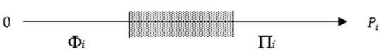
Figure 4.
Pruning regions.
Suppose is the smallest value in Πi. Because no job chooses level i with , all of the prices that are higher than will end up with the same result, that is, there are no jobs that will choose level i. Therefore, we only need to consider and prune Πi. Similarly, we only need to consider the largest value in Φi and can, therefore, prune Φi.The key issue is how to find the boundary of these regions (i.e., the smallest of Πi and the largest of Φi).
This section explains the pruning rules for a two-service-level system as an example, and presents general cases later. For a system with two levels, this section suggests the following four pruning rules in Figure 5, which have two rules for each service level.
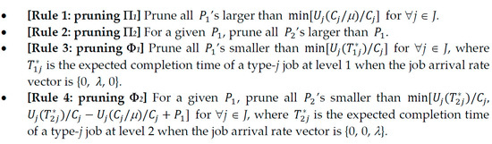
Figure 5.
Pruning rules for a system with two service levels.
Rules 1 and 2 have the following meanings: if there is no queuing delay, the minimum expected completion time is , and the maximum utility of a type-j job is . Thus, if is greater than the maximum utility value for all jobs (i.e., if for all ), then level 1 will not be selected. By contrast, if is greater than , level 2 will not be selected, because jobs in level 1 have priority over jobs in level 2 under SPS and thus no one will pay more for level 2.
Rule 3 prunes all ’s, which guarantees that all jobs will choose level 1. The highest price of the level 1 to guarantee that all of the jobs select level 1 is (i.e., for all ), where is the expected completion time of a type-j job at level 1 when the job arrival rate vector is {0, λ, 0}. can be computed using Equation (1).
Rule 4 prunes all ’s, which guarantees that all jobs choose level 2. The first condition for this scenario is for all , where is the expected completion time of a type-j job at level 2, when the job arrival rate vector is {0, 0, λ}. Another condition is for all j. Here, for the first user choosing level 1 is (i.e., zero queuing delay). Therefore, the largest should be for all j.
The pruning rules for a system with I service levels are generalized as shown in Figure 6.
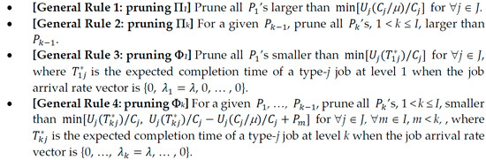
Figure 6.
Pruning rules for a system with I service levels.
5.2. Heuristic Search
After pruning has been performed, the algorithm explores the remaining search space using the heuristic search method. The algorithm adopted the “iterative-deepening” search [39], which combines the benefits of performing both a depth-first search and breadth-first search. The process begins by coarsely selecting the price vectors from the search space and then gradually tries out the other price vectors, while increasing the granularity of prices until either the computational time limit has been exhausted or the pre-set search depth limit has been reached. The algorithm also stops if the improvements between the results are negligibly small. The pseudocode for the search algorithm is shown in Figure 7.
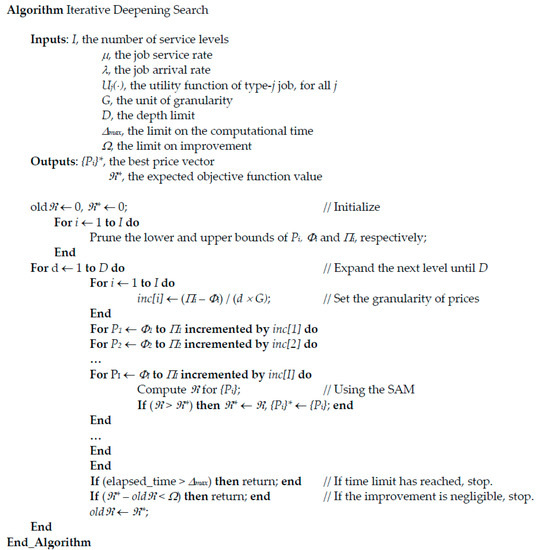
Figure 7.
Iterative deepening search algorithm.
Let us compute the system objective value for a given price vector as follows: First, SAM produces a state-transition graph. If the system converges to a steady state, then we need to account for only that state when computing the system objective value. If the system oscillates, the system objective value can be obtained by computing the weighted average of the system objective values of all states in the oscillation loop.
Another heuristic is the hill-climbing search. In general, the hill-climbing search can find the optimal solution if the objective function is unimodal (i.e., when a proper maximum is in a given region). Owing to the risk of oscillation, unimodality with respect to the price vector is not guaranteed, and the existence of local optima is possible. Techniques such as simulated annealing and multi-criteria decision analysis may be used to avoid settling into a local optimum or evaluate conflicting criteria of price and QoS, but this study does not deal with them.
Let us compute the system objective value for a given price vector {} by utilizing the SAM result as follows: SAM produces a state-transition graph. If the system converges to a steady state, we need to account for only that state when computing the system objective value. If the system oscillates, the system objective value can be obtained by computing the weighted average of the system objective values of all states in the oscillation loop. For instance, in a profit-maximization system, when the system converges to a steady state of the job arrival rate vector , the system objective function (i.e., the total system profit) is the sum of revenues collected at all service levels minus the fee that the service provider pays to his upper-level service provider:
where C is the average job size (i.e., ), where Prob(j) is the probability that a job is of type j. Note that the use of C may be approximate when some jobs are not sent. However, when the jobs not sent have an average size similar to the jobs sent, it is a good approximation. The system objective function in the case of system oscillation is calculated as follows:
where {S} denotes the set of recurring states in the oscillation loop, W(S) is the stationary probability of state S, and is the job arrival rate at level i in state S.
5.3. Example 1
This example considers a network with two service levels (I = 2). There are 10 types of jobs (J = 10), all of which have linear utility functions with a common maximum value β and a different delay cost for each job type (i.e., ). β is 10, and = 1.0, = 1.2, …, = 3.0. The total job arrival rate was set to 5.0, and the job service rate was set to 6.0. The size of the job is set to 1.0, for all job types ( = 1.0), and the base service price is set to 1.0. These parameters are designed to roughly mimic 5G mobile Internet access when users concurrently download big files from a server at maximum speed. In this setting, each job is accessing a server, and users are charged by the number of jobs they submit. According to empirical measurements in Korea [40], the average download speed of 5G mobile networks is approximately 700 Mbps and the average capacity of a base station is approximately 4.5 Gbps. Therefore, setting to 6.0 corresponds to the total capacity of 4.2 Gbps, which is about the capacity of a base station.
Figure 8 illustrates the results of search space pruning in this setting. The dotted area indicates the remaining search space after pruning, and the four lines indicate the boundary of each region defined by the four pruning rules. Rule 1 prunes out larger than , which is . As a result, the upper bound defined by Rule 1 is 9.5. Rule 2 ensures that the pruning of is larger than . Rule 3 prunes up to . The utility function is the smallest when j = 10. As a result, the lower bound of defined by Rule 3 is 7.0. Rule 4 computes the lower bound of for a given . For example, when is 9.0, is 7.0 and is (7.0 − 9.5 + 9.0). Therefore, the corresponding lower bound of is 6.5, when is 9.0.
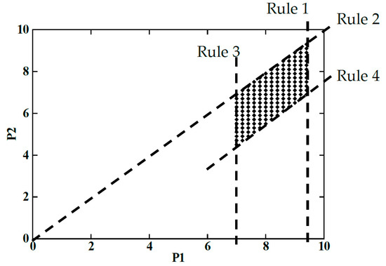
Figure 8.
Search space pruning in example 1.
The effectiveness of pruning is determined by the diversity of the utility functions. In general, the wider the distribution of utility functions, the larger the remaining region after pruning. Figure 9 compares the size of the remaining search space after pruning for two different ranges. Except the range, the setting is the same as that in Figure 8.
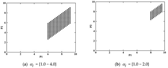
Figure 9.
The impact of utility functions on pruning efficiency
Now, let us examine how the system behaves in the pruned zone and in the remaining zone. Assume that the system objective is maximizing the system profit, so that the system objective function is . SAM is used to obtain the job arrival rate vector for a given price vector. Let us set the frequency of updates to 10 times per second. According to Rule 3, all P1′s smaller than 7.0 belong to the pruned zone and those larger than 7.0 belong to the remaining zone. Figure 10 illustrates the system behavior of the former case, and Figure 11 illustrates that of the latter case.
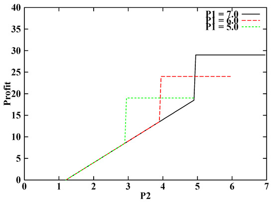
Figure 10.
System behavior in the pruned zone.
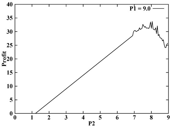
Figure 11.
System behavior in the not-pruned zone.
Figure 10 illustrates that for the price vectors belonging to the pruned zone, the system always converges on either a scenario that all jobs choose level 1 or a scenario that all jobs choose level 2. For instance, in the case of P1 = 7.0, if P2 is smaller than 5.0, all jobs choose level 2. If P2 is larger than 5.0, all jobs choose level 1. The system objective value (i.e., the system profit) in the case that all jobs choose level 1 is . The profit in the case that all jobs choose level 2 is . The highest system objective value for the pruned zone was (7.0 × 5.0 − 1.0 × 6.0) = 29.0.
Figure 11 illustrates that the system does not necessarily converge to a stable state if the price vector belongs to the unpruned zone. Rule 4 determines the range of for a given . In the case of = 9.0, P2 below 6.5 always converges on a scenario that all jobs choose level 2 so that it can be pruned (see the straight line in Figure 11). However, the system oscillates for above 6.5, and the system objective cannot be trivially computed (see the rugged line in Figure 11). My scheme applies the iterative-deepening search on the unpruned region and obtains the best price vector of {= 8.90, = 8.00}. The corresponding expected profit is 35.04. The parameters for the iterative-deepening search were set as G = 10, D = 5, Δmax = ∞, and Ω = 0. The equilibrium methods utilized about 83% of the network capacity because of the oscillation, but the proposed method let users fully utilize the capacity in this example.
5.4. Example 2
This example compares the algorithm with an equilibrium method (Case I in Section 4). Recall that Case I uses the profit maximization scheme with a single service level. The main comparison targets are the price vector and the expected system objective value. The comparison results are summarized in Table 6 and Table 7. Three system objective values, namely , of the equilibrium method, and of the heuristic search, are compared. is the system objective value (i.e., the system profit) achievable at the optimal equilibrium state as follows (assuming the system converges on the equilibrium state):
where is the job arrival rate at the equilibrium. is the system objective value computed from the SAM result using Equation (16), without assuming equilibrium.
Table 6.
Large capacity networks with frequent arrival rate broadcast (F = 100).
Table 7.
Small capacity networks with infrequent arrival rate broadcast (F = 5).
Table 6 presents the two observations. First, of the equilibrium method matches well. This is expected because I have already shown in Section 4 that the equilibrium method accurately models the actual system behavior in large capacity networks with frequent arrival rate updates. Second, of the algorithm is also very close to . These results validate the accuracy of the proposed algorithm.
Table 7 shows very different results. First, of the equilibrium method is lower than . This is because the system fails to converge to a steady state and the oscillation drops the overall system utilization (i.e., fewer jobs are submitted than the equilibrium model estimated), which decreases the system profit for the same price. Second, the price derived from the algorithm is higher than the price derived from the equilibrium method, which is due to the lack of accurate knowledge of the current system state from the user side. As the system oscillates, it broadcasts a low arrival rate and a high arrival rate. The low arrival rate makes the users underestimate the job completion delay, and the users are willing to submit their jobs even for a higher price. When the job arrival rate rises as a result of users’ decisions, the expected job completion delay increases, and the users decide not to submit their jobs. Third, from the system profit viewpoint, the gain from high price is more than enough to compensate the loss from the lower overall system utilization. Therefore, the of the algorithm is higher than that of the equilibrium. In essence, the profit-maximizing network takes advantage of the users who do not have up-to-date knowledge of the system status.
5.5. Example 3
This example compares the algorithm with another equilibrium method (Case II in Section 4). Case II uses a net-value maximization scheme with a single service level. As in Example 2, the comparison targets are the price vector and the expected system objective value. The comparison results are summarized in Table 8 and Table 9. is the system objective value (i.e., the system net value or social welfare) computed at the optimal equilibrium state as follows:
where L is the mean number of jobs, and λ* is the job arrival rate in the equilibrium state. is the system objective value computed from the SAM result using the following equation:
where {S} denotes the set of recurring states in the SAM transition graph, W(S) is the stationary probability of state S, is the job arrival rate in state S, V′ is the marginal value function, and T(S) is the average job completion time in state S.
Table 8.
Large capacity networks with frequent arrival rate broadcast (F = 100).
Table 9.
Small capacity networks with infrequent arrival rate broadcast (F = 5).
Table 8 offers the same observations as those in Table 6. The equilibrium method accurately models the actual system behavior in large capacity networks with frequent arrival rate updates, and as a result, the outcome of the algorithm matches that of the equilibrium method.
Table 9 is similar to Table 7, with a few differences. First, of the equilibrium method is lower than . Unlike in Example 2 (the profit-maximizing network), of the algorithm is also lower than . This is because the sub-optimal decisions of users, owing to inaccurate knowledge of the system status, do not increase the system objective value in the net-value-maximizing network. Nonetheless, the algorithm results in higher values than the equilibrium method and achieves a system objective closer to the theoretical maximum value . Second, the sensitivity to price is generally lower than that in the profit-maximizing network because the price that generates the highest is not a single point but rather a range of prices. This occurs because the system objective function is not directly affected by the price (see Equation (17)). As long as the system stays in the same state or the same set of states (i.e., has the same job arrival rate), the system objective value is the same regardless of the price.
6. Conclusions
This study investigates the practicality of using equilibrium analysis to address the price selection problem. Results showed that certain conditions that are needed to produce a stationary equilibrium may not hold in real networks; consequently, the system may oscillate instead of converging on the equilibrium. I demonstrated that when such conditions are not met, the system oscillates among a number of states without reaching a static equilibrium. I also showed that the price vectors computed by the equilibrium methods are suboptimal when the system fails to converge on a static equilibrium. As an alternative, I developed a new price selection method that does not rely on an equilibrium analysis. My findings suggest a need for more realistic modeling of the system dynamics to solve the price selection problem.
In future investigations, the multi-criteria decision analysis and simulated annealing search for the price selection problem would be worthy research topics.
Funding
This research received no external funding.
Conflicts of Interest
The author declares no conflict of interest.
References
- International Telecommunication Union. Measuring Digital Development. ICT Price Trends 2019; International Telecommunication Union Place des Nations: Geneva, Switzerland, 2020. [Google Scholar]
- Asadi, A.; Sciancalepore, V.; Mancuso, V. On the Efficient Utilization of Radio Resources in Extremely Dense Wireless Networks. IEEE Commun. Mag. 2015, 53, 126–132. [Google Scholar] [CrossRef]
- He, H.; Xu, K.; Liu, Y. Internet resource pricing models, mechanisms, and methods. Netw. Sci. 2012, 1, 48–66. [Google Scholar] [CrossRef]
- Odlyzko, A. Internet Pricing and the History of Communications. Comput. Netw. 2001, 36, 493–517. [Google Scholar] [CrossRef]
- Zhang, L.; Wu, W.; Wang, D. Time Dependent Pricing in Wireless Data Networks: Flat-rate vs. Usage-based Schemes. In Proceedings of the IEEE INFOCOM 2014—IEEE Conference on Computer Communications, Toronto, ON, Canada, 27 April–2 May 2014; pp. 700–708. [Google Scholar]
- An Architecture for Differentiated Services. IETF RFC 2475. Available online: https://tools.ietf.org/html/rfc2475 (accessed on 31 March 2021).
- New Terminology and Clarifications for Diffserv. IETF RFC 3260. Available online: https://tools.ietf.org/html/rfc3260 (accessed on 31 March 2021).
- Differentiated Services (Diffserv) and Real-Time Communication. IETF RFC 7657. Available online: https://tools.ietf.org/html/rfc7657 (accessed on 31 March 2021).
- System Architecture for the 5G System (5GS). Stage 2 (Release 16). 3GPP TS 23.501. Available online: https://portal.3gpp.org/desktopmodules/Specifications/SpecificationDetails.aspx?specificationId=3144 (accessed on 31 March 2021).
- Cocchi, R.; Shenker, S.; Estrin, D.; Zhang, L. Pricing in Computer Networks: Motivation, Formulation, and Example. IEEE/ACM Trans. Netw. 1993, 1, 614–627. [Google Scholar] [CrossRef]
- Cao, P.; Wang, Y.; Xie, J. Priority Service Pricing with Heterogeneous Customers: Impact of Delay Cost Distribution. Prod. Oper. Manag. 2019, 28, 2854–2876. [Google Scholar] [CrossRef]
- Mackie-Mason, J.; Varian, H. Pricing Congestible Network Resources. IEEE J. Sel. Areas Commun. 1995, 13, 1141–1149. [Google Scholar] [CrossRef]
- Mackie-Mason, J. A Smart Market for Resource Reservation in a Multiple Quality of Service Information Network; Technical Report; University of Michigan: Ann Arbor, MI, USA, 1997. [Google Scholar]
- Odlyzko, A. A Modest Proposal for Preventing Internet Congestion; Technical Report; AT&T Center for Discrete Mathematics & Theoretical Computer Science: Piscataway, NJ, USA, 1997. [Google Scholar]
- Passas, V.; Miliotis, V.; Makris, N.; Korakis, T. Pricing Based Distributed Traffic Allocation for 5G Heterogeneous Networks. IEEE Trans. Veh. Technol. 2020, 69, 12111–12123. [Google Scholar] [CrossRef]
- Chod, J.; Rudi, N. Resource Flexibility with Responsive Pricing. Oper. Res. 2005, 53, 532–548. [Google Scholar] [CrossRef]
- Shenker, S.; Clark, D.; Estrin, D.; Herzog, S. Pricing in Computer Networks: Reshaping the Research Agenda. ACM Comput. Commun. Rev. 1996, 26, 19–43. [Google Scholar] [CrossRef]
- Karakostas, G.; Kolliopoulos, S.G. Edge Pricing of Multicommodity Networks for Selfish Users with Elastic Demands. Algorithmica 2009, 53, 225–249. [Google Scholar] [CrossRef]
- Kelly, F.; Maullo, A.; Tan, D. Rate Control for Communication Networks: Shadow Prices, Proportional Fairness and Stability. J. Oper. Res. Soc. 1998, 49, 237–252. [Google Scholar] [CrossRef]
- Cho, S.; Goel, A. Pricing for Fairness: Distributed Resource Allocation for Multiple Objectives. Algorithmica 2010, 57, 873–892. [Google Scholar] [CrossRef]
- Mandjes, M. Pricing Strategies under Heterogeneous Service Requirements. Comput. Netw. 2003, 42, 231–249. [Google Scholar] [CrossRef]
- Mendelson, H. Pricing Computer Services: Queuing Effects. Commun. ACM 1985, 28, 312–321. [Google Scholar] [CrossRef]
- Mendelson, H.; Whang, S. Optimal Incentive-Compatible Priority Pricing for the M/M/1 Queue. Oper. Res. 1990, 38, 870–883. [Google Scholar] [CrossRef]
- Keon, N.; Anandalingam, G.A. A New Pricing Model for Competitive Telecommunications Services Using Congestion Discounts. INFORMS J. Comput. 2005, 17, 248–262. [Google Scholar] [CrossRef]
- Zhang, Z.; Dey, D.; Tan, Y. Price and QoS competition in data communication services. Eur. J. Oper. Res. 2008, 187, 871–886. [Google Scholar] [CrossRef]
- Li, L.; Siew, M.; Quek, T.Q.S.; Ren, J.; Chen, Z. Optimal Pricing for Job Offloading in the MEC System with Two Priority Classes. arXiv 2019, arXiv:1905.07749. [Google Scholar]
- Lee, D.H. Optimal Pricing Strategies and Customers’ Equilibrium Behavior in an Unobservable M/M/1 Queueing System with Negative Customers and Repair. Math. Probl. Eng. 2017, 2017, 1–11. [Google Scholar] [CrossRef]
- Wang, J.; Cui, S.; Wang, Z. Equilibrium Strategies in M/M/1 Priority Queues with Balking. Prod. Oper. Manag. 2019, 28, 43–62. [Google Scholar] [CrossRef]
- Park, S. Analysis of the Price-Selection Problem in Priority-based Scheduling. J. KIISE 2006, 33, 183–192. [Google Scholar]
- Low, S.; Lapsley, D. Optimization Flow Control – I: Basic Algorithm and Convergence. IEEE/ACM Trans. Netw. 1999, 7, 861–874. [Google Scholar] [CrossRef]
- Balachandran, K.; Srinidhi, B. A Rationale for Fixed Charge Application. J. Account. Audit. Finance 1987, 15, 151–169. [Google Scholar] [CrossRef]
- Hassin, R. Consumer Information in Markets with Random Products Quality: The Case of Queues and Balking. Econometrica 1986, 54, 1185–1195. [Google Scholar] [CrossRef]
- Armony, M.; Shimkin, N.; Whitt, W. The Impact of Delay Announcements in Many-Server Queues with Abandonment. Oper. Res. 2009, 57, 66–81. [Google Scholar] [CrossRef]
- Dighriri, M.; Alfoudi, A.S.D.; Lee, G.M.; Baker, T.; Pereira, R. Comparison Data Traffic Scheduling Techniques for Classifying QoS over 5G Mobile Networks. In Proceedings of the 31st International Conference on Advanced Information Networking and Applications Workshops (WAINA), Taipei, Taiwan, 27–29 March 2017; pp. 492–497. [Google Scholar]
- Bertsekas, D.; Gallager, R. Data Networks; Prentice-Hall: Englewood Cliffs, NJ, USA, 1992. [Google Scholar]
- Kumar, A.; Manjunath, D.; Kuri, J. Wireless Networking; Morgan Kaufmann: Burlington, MA, USA, 2008. [Google Scholar]
- Jindal, A.; Psounis, K.; Liu, M. CapEst: A Measurement-Based Approach to Estimating Link Capacity in Wireless Networks. IEEE Trans. Mob. Comput. 2012, 11, 2098–2108. [Google Scholar] [CrossRef]
- Keshav, S. An Engineering Approach to Computer Networking; Addison Wesley: Boston, MA, USA, 1997. [Google Scholar]
- Russell, S.; Norvig, P. Artificial Intelligence: A Modern Approach; Pearson: Hoboken, NJ, USA, 2020. [Google Scholar]
- 2020 Communication Service Coverage Check and Quality Evaluation Report. Ministry of Science and ICT Korea. Available online: https://www.msit.go.kr/bbs/view.do?sCode=user&mId=113&mPid=112&bbsSeqNo=94&nttSeqNo=3012555 (accessed on 31 March 2021).


Publisher’s Note: MDPI stays neutral with regard to jurisdictional claims in published maps and institutional affiliations. |
© 2021 by the author. Licensee MDPI, Basel, Switzerland. This article is an open access article distributed under the terms and conditions of the Creative Commons Attribution (CC BY) license (https://creativecommons.org/licenses/by/4.0/).