Abstract
Mobile Edge Computing (MEC) has emerged as a promising network computing paradigm associated with mobile devices at local areas to diminish network latency under the employment and utilization of cloud/edge computing resources. In that context, MEC solutions are required to dynamically allocate mobile requests as close as possible to their computing resources. Moreover, the computing power and resource capacity of MEC server machines can directly impact the performance and operational availability of mobile apps and services. The systems practitioners must understand the trade off between performance and availability in systems design stages. The analytical models are suited to such an objective. Therefore, this paper proposes Stochastic Petri Net (SPN) models to evaluate both performance and availability of MEC environments. Different to previous work, our proposal includes unique metrics such as discard probability and a sensitivity analysis that guides the evaluation decisions. The models are highly flexible by considering fourteen transitions at the base model and twenty-five transitions at the extended model. The performance model was validated with a real experiment, the result of which indicated equality between experiment and model with p-value equal to 0.684 by t-Test. Regarding availability, the results of the extended model, different from the base model, always remain above 99%, since it presents redundancy in the components that were impacting availability in the base model. A numerical analysis is performed in a comprehensive manner, and the output results of this study can serve as a practical guide in designing MEC computing system architectures by making it possible to evaluate the trade-off between Mean Response Time (MRT) and resource utilization.
1. Introduction
Mobile devices have changed the way people live in the last years. According to the Statista (a German online portal for statistics), the number of mobile devices will be around 16.8 billion in 2023 [1]. Unfortunately, mobile devices still present limited resources in terms of battery lifetime, storage, and processing capacity. Cellular networks must support low storage capacity, high power consumption, low bandwidth, and high latency [2]. Besides, the exponential growth of the Internet of Things (IoT) promises to make wireless networks even more challenging [3,4].
Many previous studies proposed optimized architectures for this context, such as Mobile Cloud Computing (MCC) [5,6,7]. MCC is the integration of cloud computing and mobile computing, which provides additional capabilities for mobile devices by centralizing their resources in the cloud [8]. The technique, called offloading, can transfer resource-intensive tasks to remote clouds. MCC can reduce latency problems by providing a secure and efficient model. However, cloud resources are often far away from end-users [9]. Thus, with multiple mobile devices, MCC faces notable challenges, such as high latency, security vulnerability, and limited data transmission.
Mobile Edge Computing (MEC) has emerged as a more efficient alternative to MCC architecture. The main goal of MEC is to address the challenges that MCC has been facing, deploying resources even closer to users—at the edge of the network. Thus, computing and storage are performed closer to the source device [10]. MEC aims to enable the billions of connected mobile devices to execute the real-time compute-intensive applications directly at the network edge. The distinguishing features of MEC are its closeness to end-users, mobility support, and dense geographical deployment of the MEC servers [11]. Since MEC is still considered a recent topic, some research gaps still have to be explored, such as performance evaluation of MEC architectures.
Availability evaluation is another topic of interest in the MEC area. MEC was designed to provide services in real-time, and therefore, robustness and availability are essential requirements, since the resources are close to the clients, providing them critical services. All components of a system are prone to failure, and failures must be repaired as soon as possible. Assessing the availability of a MEC architecture can be costly, considering practical experiments. Thus, it is necessary to evaluate MEC architectures even before a real deployment, using analytical models, for example.
Therefore, there is a lack of studies evaluating MEC architectures through analytical models in terms of performance and availability. Stochastic Petri nets (SPN) [12,13] are analytical models capable of representing concurrency, synchronization, and parallelism of complex systems. Among other metrics, SPN are well suited to evaluate performance and availability [14,15,16]. The use of SPNs has already been successfully applied in the context of MCC in previous works [17,18,19]. However, SPNs representing MEC architectures are scarce until the present moment. This paper presents SPN models to evaluate MEC architecture with significant difference to the literature, including sensitivity analysis and unique metrics, such as discard probability of requests and resource utilization level. The proposed models allow evaluating the trade-off between MRTand resource utilization, besides the availability and downtime of the system. In summary, the main contributions of this paper are:
- SPN models, which are useful tools for system administrators to evaluate the performance and availability of MEC architectures, even before they are deployed. Other types of models could be used, for example the Markov Chains, however, SPNs are equivalent to these models with higher representativeness;
- Sensitivity analysis under the SPN models parameters to identify the most important components;
- Case studies that provide a practical guide to performance and availability analysis in MEC architectures.
The remainder of this paper is divided as follows: Section 3 presents the MEC architecture, considered to design the SPN models. Section 4 presents performance SPN models, with respective metrics, case studies, and validation. Section 5 presents SPN availability models (including redundancy) case studies and a sensitivity analysis under the model components. Section 2 discusses the main related works; and Section 6 traces some conclusions and future works.
2. Comparison with Related Work
This section presents some related works. Table 1 summarizes all the compared papers. Fourteen papers were found using the keywords that matched this proposal. The papers were divided, taking into account five aspects: Metrics, capacity variation of the master–slave server, sensitivity analysis, context, and use of component dependency.

Table 1.
Related works.
Metrics—Metrics help to compute and subsequently understand the behavior of a system. This paper uses metrics of both performance and availability that were not explored together by any other previous article. Among the works that deal with performance at the edge, only this work used the metrics MRT, resource utilization, and drop probability. The work of [26,27,28,29,30,31,32] focused solely on system availability, but as we will see later, only the work of [32] focuses on the edge, as this work.
This work presents a very unique edge architecture, and because of that, another contribution of this work is to do experiments with Capacity variation of the master-slave server. Among the related works, no work used the architecture used here, which provides a greater number of parameters. This work also performs a Sensitivity analysis that allows the identification of the key components for the architecture and, consequently, for the model. Among the works found, only the works of [27,31] performed a sensitivity analysis. However, the work of [27] was in a Cloud context, while the work of [31] presents an edge context, but focused specifically on the area of smart hospitals.
Context—all papers are in the context of remote computing, whether in the cloud, on the edge, or in the fog. Most works focus on edge architecture, however, most of them are aimed at measuring edge energy consumption. Unlike these works, our work uses metrics that have not been explored in this context so far. The work of [32] is the only one related to availability that focuses exclusively on the edge.
Finally, use of component dependency is a unique contribution. The technique is still little explored, but it is essential to ensure the correct functioning of the system as a whole. The technique is applied to Petri net models to ensure that if a component that is the basis for other components falls, it causes a cascade effect to turn off those components that depend on it. Thus, it can be guaranteed that an availability model will be as close to reality as possible, and only this work made use of this aspect of the Petri nets in modeling the availability of the system.
3. Architecture Overview
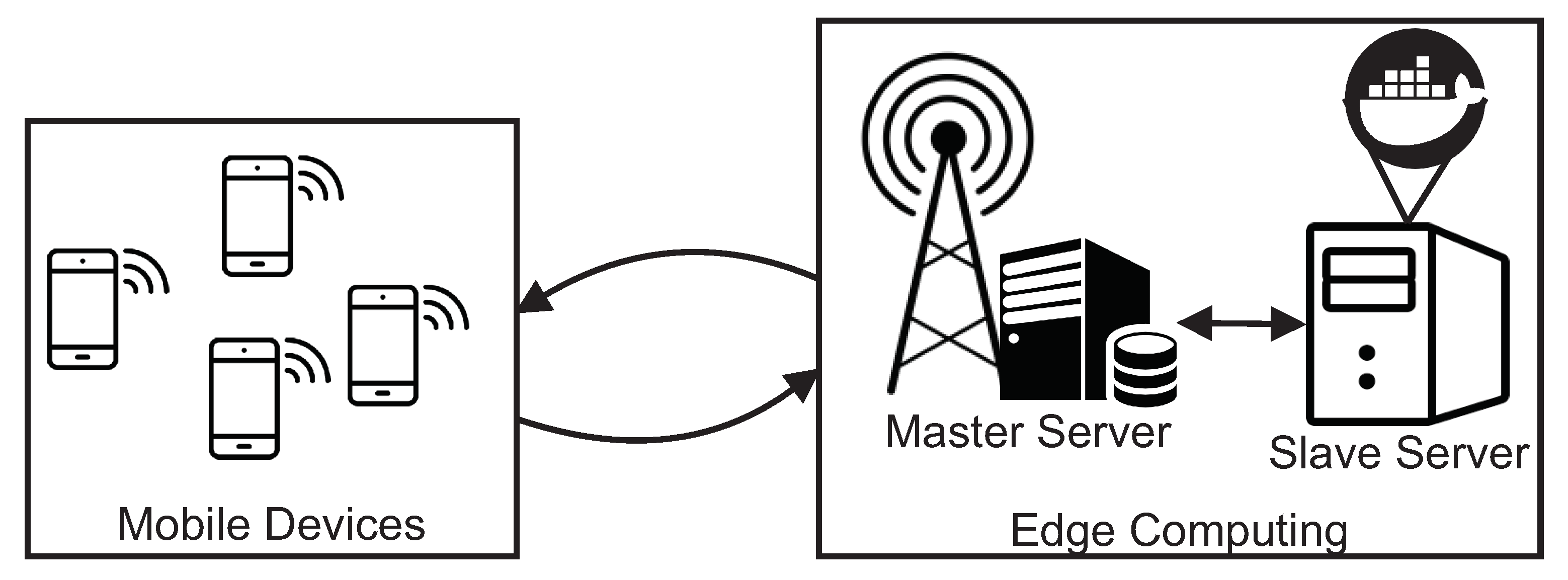
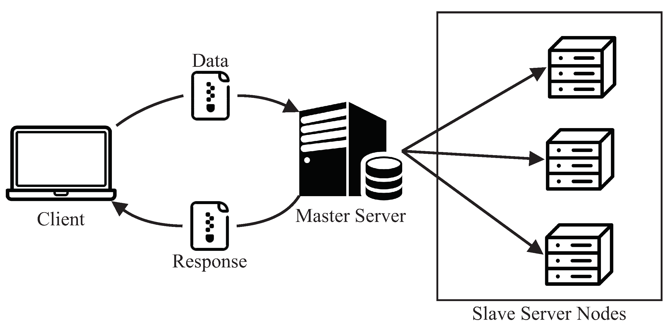
Figure 1 illustrates the proposed MEC architecture that was considered to construct the SPN model. Such a base architecture is widely adopted to describe the MEC infrastructure in several works [21,33,34] with a MEC server for processing incoming data streams. These data are generated and sent by applications running on mobile devices, for example, user-health monitoring applications, game rendering, etc. In the context of this work, we focus on applications with a high level of user interactivity, including peripherals such as smartphones or tablets.
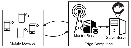
Figure 1.
MEC Architecture Base Adopted in Performance Evaluation. (adapted from [35,36]).
In more detail, in the edge computing layer, we have two servers, a master server and a server with the slave nodes (which will perform the processing itself). Slaves are micro-services that run in containers. In this work, each container is configured to run on a server core. Therefore, if there are 16 cores, 16 containers will be executed. The use of containers in the MEC context is still not very common. The use of containers allows greater flexibility to scale the computational power of the architecture according to the volume of tasks and also restrictions of applications’ response times.
The master server is responsible for receiving requests from mobile devices and distributing them between slave servers. At first, the master server runs the management service with the service running in bare metal (non-virtualized) mode and using threads. However, nothing prevents the analyst from virtualizing the master server service as well. To manage the containers, we consider that a container orchestrator (e.g., Kubernetes (Kubernetes: https://kubernetes.io/, accessed on 20 December 2020) or Swarm (Swarm: https://docs.docker.com/engine/swarm/, accessed on 25 December 2020)) should be used to increase resources reliability and elasticity.
As Figure 2 illustrates, there are three blocks in the communication flow of the architecture: (i) Arrival Delay (AD): time interval between arrivals of requests; (ii) Distribution Delay (DD): time interval for distributing jobs; and (iii) Processing Delay (PD): processing time of the requests by the nodes.

Figure 2.
Communication Time Intervals for the Architecture Components. (adapted from [35,36]).
Recent advances in the invention and fabrication of new lines of mobile devices help ease people’s daily activities with a tremendous number of mobile apps, which feature a huge amount of stream-like data transactions through limited connection bandwidths and mobile computing resources. In such a busy context, MEC, as shown in Figure 1, can enhance and secure a high level of quality of service (QoS) in terms of performance and availability to mobile users. The MEC architecture aims to take advantages of edge computing power and resources at near-by places to resolve inherent limitations of mobile computing, enabling the hosting and uninterrupted delivery of heavy mobile apps and stream-like services that often consume huge amount of computing power and resources to mobile users. As a critical requirement, comprehensive modeling and assessment of such MEC architectures are of paramount importance for planning and development of mobile devices and services in practice.
4. Evaluation of MEC Performance
This section presents two models for evaluating the performance of MEC architecture. In addition to the models, their respective case studies, metrics, and validation will be presented.
All the evaluations, including performance and availability models, were solved by numerical analysis. Usually, the numerical analysis is preferred instead of simulation because it offers a greater accuracy in the results [37]. Therefore, the evaluator must try first the possibility of using numerical analysis but sometimes it is not possible. Petri Nets and Markov Chains can present the problem known as “state-space explosion” if the model is too big. In our case, fortunately the model can be solved by numerical analysis.
4.1. Basic SPN Model for MEC Architectures
In this section, we describe our SPN model to represent the architecture that integrates modules at the edge of the network, presented in the previous section. We emphasize that the purpose of our model is to make it possible to evaluate system performance, even before they are implemented. Figure 3 presents our SPN model, composed of two macro parts:

Figure 3.
SPN Model for an Edge Computing Architecture.
- Admission, which deals with the generation of requests;
- Edge, composed of the master server and the server with slave nodes. The master server receives data and distributes it between slaves, which ultimately return the results to clients.
In an SPN model, fundamental graphical elements are used to represent system components, for instance, empty circles, filled circles, and empty bars represent places, place markings, and places in SPN model, respectively. The model elements are all described in Table 2. Probability distributions are associated with timed transitions in the SPN model to capture the sojourn time of an event. To associate different probability distributions, the person in charge of system administration needs to investigate in the literature or conduct experimental measurements/characterizations of the system.

Table 2.
Description of the Model Elements.
The description of the model and its flow of data processing throughout its components is as follows. Two places, P_Arrival and P_InputQueue, in the Admission sub-net capture the waiting behaviors between the generation and the acceptance of requests in the queue, respectively. Tokens which reside in the two places, P_Arrival and P_InputQueue, represent the involvement of data entry for any type of requests. The transition AD is used to capture the time between request arrivals. AD means arrival delay. We assume that times between arrivals comply with exponential distribution. However, this assumption is possibly relaxed considering other type of probability distribution. The AD transition does not take into account network losses.
As soon as T0 is enabled, requests arrive at the Edge sub-net. The queuing and amount of requests on edge are represented by the deposit and the number of tokens in P_MasterInProcess. The MC mark in P_MasterCapacity indicates the amount of temporary storage space of the master server, queuing the requests. In the case that capacity for processing requests in the master and slave is not sufficient for newly arrived requests, those requests are continuously queued. Thus, shortly after an amount of storage space is released, a token from P_InputQueue and P_MasterCapacity each is taken out and then deposited in P_MasterInProcess. When this happens, the place P_Arrival is then enabled, allowing a new arrival.
DD firing represents the beginning of the distribution of requests to the slaves. DD means distribution delay. These firings are conditioned to the amount of available nodes for processing in P_SlavesCapacity (with SC mark). The SC tag indicates the number of available nodes at the network edge. In the case that requests are under processing by slaves represented by tokens in P_SlavesInProcess, the tokens go out from P_SlavesCapacity. This flow means that an amount of the resource will be allocated to each arriving request.
PD represents the time spent by the slave node to process a request. When PD is fired, a token is pulled from P_SlavesInProcess, and a token is returned to P_SlavesCapacity. The AD transition has an exponential distribution since we are considering exponentially distributed arrival rates. The infinite server semantics are associated with all other transitions so that the processing of each job is independent to each other. It is worth noting that the computational capacity of each node causes an impact on the processing time. Nevertheless, we assume in this work that same computational capacity is given to all nodes in each layer.
A vast number of different scenarios can be evaluated using the proposed model, because the evaluator needs to configure five parameters as shown in Table 2. The parameters include three timed transitions and the two place-related resource or workload markings. A certain change in the value of any parameter causes a significant impact on various performance metrics such as discard level, MRT, or resource utilization. The capability to investigate the variation of different scenarios and/or a number of impacting factors makes the proposed model a main contribution of this study.
4.1.1. Performance Metrics
Performance metrics are presented in this section, which are used to evaluate the performance of the edge architecture based on its proposed SPN model. The MRT is computed by adopting the Little’s law [38]. Little’s law takes into account the number of ongoing requests in a system ()—mean system size, the arrival rate of new requests (), and the MRT. The arrival rate is the inverse of the arrival delay—that is, . A stable system is required to compute metrics based on Little’s law. It means that the arrival rate must be lower or equal than the server processing rate. We assume that the actual arrival rate can be different with the effective one, or discarded due to finite queue size. Then, to obtain the effective arrival rate, we multiply the arrival rate () by the probability for the system to accept new requests () [39]. Therefore, Equation (1) obtains considering Little’s law and the effective arrival rate.
Equation (2) obtains . To compute the number of ongoing requests in the system, the analyst must compute the sum of the expected number of tokens, which is deposited in each place representing ongoing requests. In Equation (2), represents the statistical expectation of tokens in the “Place”, where . In other words, indicates the expected mean number of tokens in that place.
Equation (3) defines . There must be one token in the input queue (P_ArrivalQueue), and there must be no more resources available to process new requests both in the master and slave nodes. computes the probability of n tokens in that “Place”.
Finally, in addition to MRT, we also calculate resource utilization. Equation (4) gives us the utilization of the master node. Equation (5) gives us the utilization of the slave nodes. The utilization is obtained by dividing the number of tokens of the corresponding place by the capacity of the total resources.
4.1.2. Numerical Analysis
This section presents two numerical analyzes for MRT, discard, and utilization evaluations. In [40], the authors evaluated a MEC architecture with a single mobile device as a client and containers executing the services. Authors have evaluated a 3D game called Neverball, where the player must tilt the floor to control the ball to collect coins and reach an exit point before the time runs out. We have considered the system parameters in [40] as input parameters for our model. Therefore, our study evolves the work in [40] by performing numerical analysis to evaluate the scenarios considering multiple parameters. We have considered one of their scenarios with a game resolution of 800 × 600 pixels. The adopted parameter value corresponding to the processing delay (PD) of a request is 24 ms. We adopted 5 ms as the time for distributing the requests in the system (DD transition). We established that the master server has a restriction regarding the maximum number of requests that may be simultaneously processed. This number corresponds to 40 requests—that is, MC = 40.
The model allows a wide variety of parameterizations. In the present analysis, we vary two parameters: the time interval between requests arrivals (AD) and the resource capacity of the server with slave (SC) nodes. The value of AD was varied between 1 ms and 10 ms, considering a step size of 0.5 ms. The SC variable was configured with three possibilities (8, 16, and 32), corresponding to the number of cores in a server. All these parameters could be varied in other ways. For example, the number of slaves could not be tied to the number of cores—SC could store thousands of tokens. Adopting the parameters mentioned above, we present the results considering MRT, discard, and utilization of the master server and slave servers.
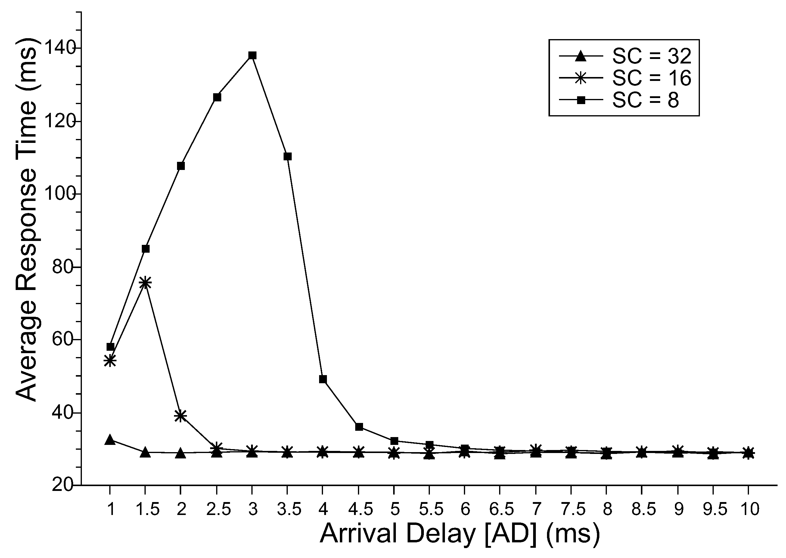
Figure 4 shows the results for the MRT. At first, it is expected that the larger the time interval between arrivals (AD), the smaller the MRT. The system will be more able to handle the incoming requests with the available processing resources. It is also expected that the higher the slave’s capacity (SC), the lower the MRT because more processing capacity is available to handle the requests. These two behaviors are easily observed when the values of discards are minimal in the model (which can be observed in Figure 7). For minimal discards, the MRT decreases until the minimum time to perform requests without requests waiting in the queue.
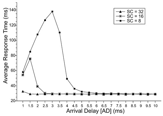
Figure 4.
MRT.
However, when the system discards incoming requests, we observe the increase of the MRT until a peak, decreasing after that. This behavior is due to the limiting value of resources in the system, where some of the incoming requests are discarded when there are no more resources available to process them. Thus, limiting the MRT variation to the time between arrivals. As can be deduced from Little’s law [39], the mean time between exits will increase along with the mean time between arrivals until to reach the peak. In our numeric results, the peaks were: for SC = 8 was in AD = 1.5 ms and for SC = 16 it was AD = 3.0 ms. At these points, the amount of work within the system begins to reduce, reducing MRT even when AD increases drastically. It is important to emphasize that in MRT, we consider the effective arrival rate, that is, adjusting its value by considering the discard probability.
The MRT for SC = 32 is low, even for a time interval between arrivals of 1 ms. Comparing SC = 16 and SC = 32, and considering an arrival delay of 2.5 ms, the MRTs equalize. Considering an arrival delay of 5.5 ms, and the SC = 8, it also presents the same average result. Therefore, if the real context has had an AD = 5.5 ms, an 8-core server would achieve the same performance as more powerful servers. Therefore, our work may assist managers in the task of choosing servers and identifying the best performance and costs, considering the expected workload.
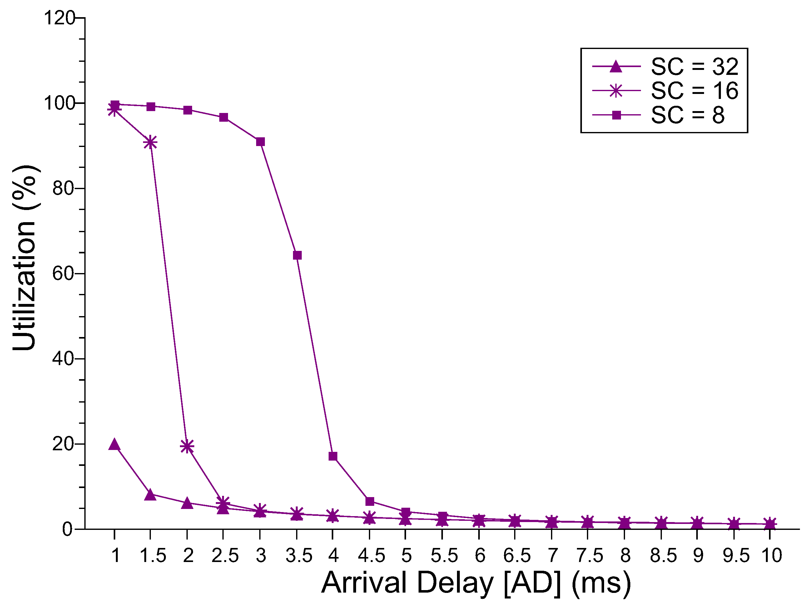
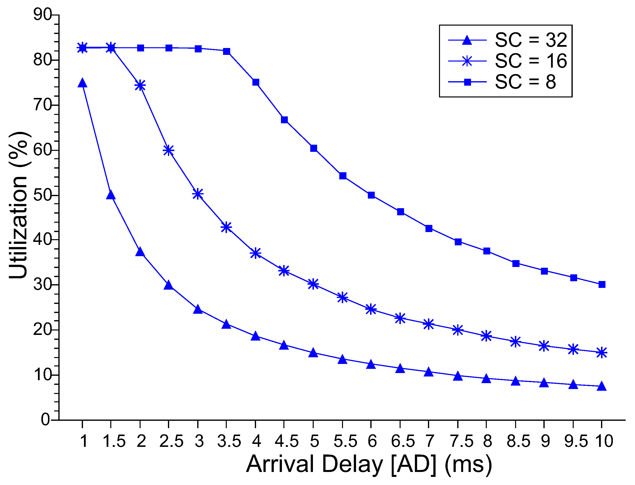
Figure 5 shows the level of utilization of the master server. The master server is the first component that the request reaches upon entering the MEC layer. For the SC = 8 and SC = 16 configurations, the utilization level is around 100% in the lowest AD values; after that, utilization drops. For SC = 32, even with AD = 1.0 ms, the utilization value reaches only 20%. From AD = 5.5 ms, the three configurations have values similar to and close to 0%. The system administrator must consider the desire for high or low idle server levels. Figure 6 shows the level of utilization of the slave servers. The higher the number of resources, the lower the level of utilization of the slaves. As AD increases, the level of utilization declines subtly in all three cases. However, this fall only starts at AD = 3.0 ms for SC = 8 and at AD = 1.5 ms for SC = 16. Up to these points, the utilization level is around 82%, which causes the behavior of the MRT explained above.
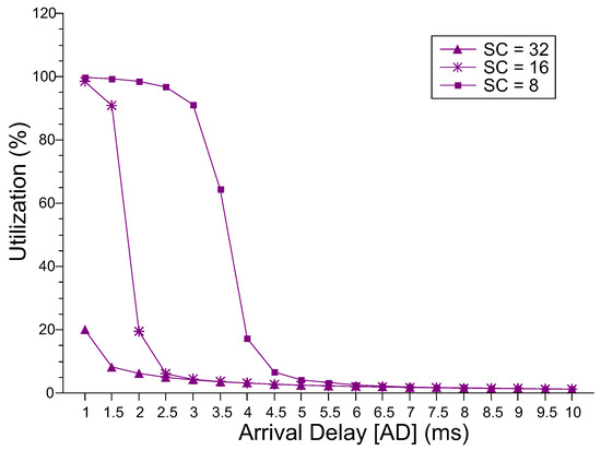
Figure 5.
Master Server Utilization Level.
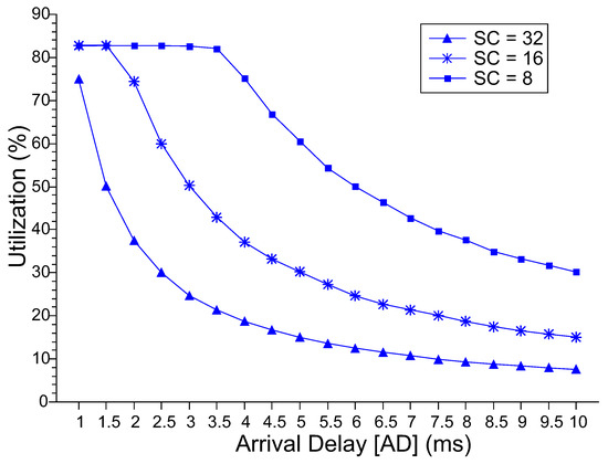
Figure 6.
Slaves Server Utilization Level.
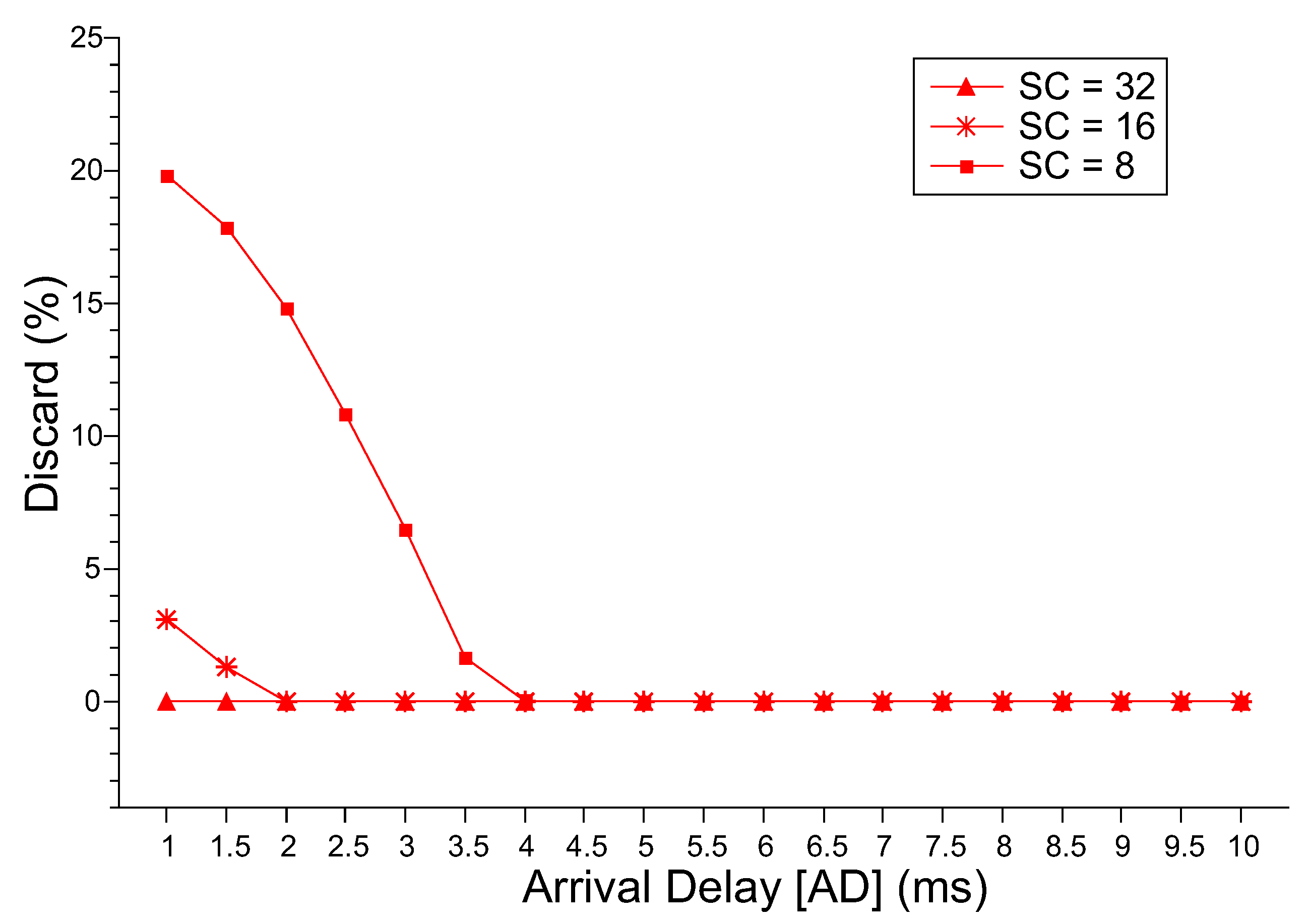
Figure 7 presents the probability of discarding new requests. For SC = 32, the discard probability is equal to 0. Therefore, if it is possible to acquire a server with 32 cores, there will be no discarding independent of the interval between request arrivals. For SC = 8 and SC = 16, only from AD = 2.0 ms and AD = 4.0, the discard probabilities tend to 0. These initial discard intervals are directly related to the high level of utilization presented by both servers, directly impacting the MRT. Therefore, any stochastic analysis performed with the proposed model must observe the four metrics to obtain a complete view of the system behavior. It is also possible to identify the operating limits of the system. In other words, these limits represent how many jobs can be lost without compromising the utility of the system.

Figure 7.
Discard Probability.
4.2. Refined Model with Absorbing State
System administrators who want to use a MEC architecture should be aware of when their applications are most likely to finish execution. Cumulative Distribution Functions (CDFs) may indicate such a moment through the maximum probability of absorption. CDFs are associated with a specific probability distribution. In this work, the probability distribution is related to the probability of finishing the application execution within a specified time. It is obtained through transient evaluation, generating probabilities with time tending to one value t. In other words, developers compute the probability of absorption in [0, t), through transient evaluation, where F (t) approaches 1.
CDFs indicate the maximum probability of an application’s processing to be completed within a given time interval. In this work, the absorbing state is reached when the model is in the FINISH state. For a better understanding of time-dependent metrics, it is necessary to define the difference between transient state and absorbing one. Transient states are defined as temporary states. In other words, when the system leaves a transient state, there is a likelihood of never coming back to it again. On the other hand, an absorbing state is a state that when the system reaches it, there is no way out. Figure 8 shows the adaptation we made in our SPN model presented previously to calculate CDFs.

Figure 8.
SPN Model Using Absorbing State.
Three changes were made: (a) an absorbing state place (named Finish) was added in the right part of the model, indicating that when the requests reach this place, such requests will not change state; (b) in the Admission block, the feedback loop () has been withdrawn, indicating that new requests will not be generated unmistakably; and (c) there is a new parameter called BATCH (at place P_Arrival) that represents the number of jobs (tokens) that will be processed. The CDF calculates the probability of these jobs to complete the application processing at a given time and in a specific time interval.
4.2.1. Case Study 1
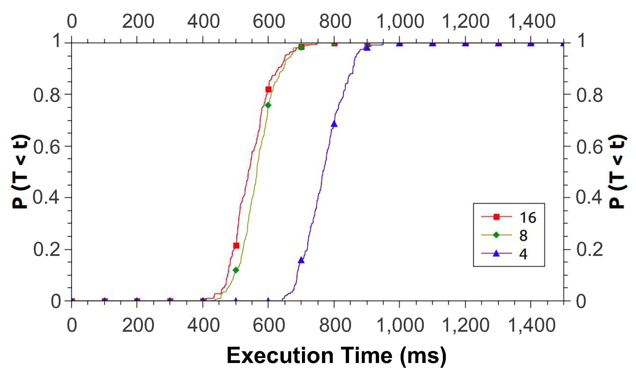
For this study, we set the master server capacity (MASTERC) as 40, the time between arrivals (AD) to 5 ms, and we created three scenarios by varying the server capacity with the slave nodes (SLAVEC) as 8, 16, and 32. These scenarios have been defined in order to verify which slave server configuration best meets the requirements of an infrastructure administrator, according to the total time desired for the application execution. Table 3 allows a better view of these variables.

Table 3.
Possible scenarios for case study 1.
Figure 9 shows the results obtained for CDF. In general, scenario #1 is the one that takes the longest time to run the application. Note that the scenarios #2 and #3 are the best cases, and with performance levels close to each other. Despite some occurrences where scenario #3 fares better than #2, when the probability of execution ends near 1, the times balance out. We can also see that both scenarios have an execution time in which the probability increases intensely. Assuming that an infrastructure administrator wants their application to complete within 800 ms, this can be accomplished using scenarios #2 and #3, and a choice can be made based on resource availability.
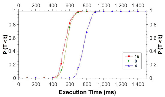
Figure 9.
Cumulative Distribution Functions for Study 1.
4.2.2. Case Study 2
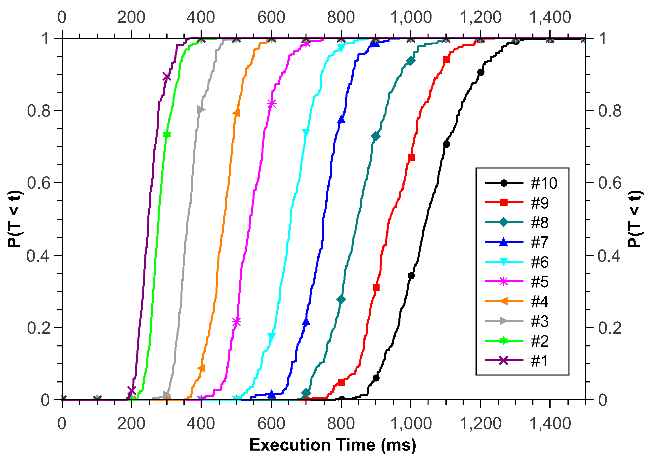
For this study, we set the master server (MASTERC) capacity to 40, the slave server capacity to 16 nodes, and create some scenarios ranging from arrival time (AD) with values between 1 ms to 10 ms, with 1 ms increments. Table 4 presents the combination of these variables.

Table 4.
Possible scenarios for case study 2.
Figure 10 presents the results obtained for the CDF metric. The application execution time increases with the increase of AD. In this study, we have a batch of 100 requests. Each of these requests enters the model according to the interval defined in AD. Thus, for AD equal to 1 ms, we know that the minimum application execution time is 100 ms, while for AD equal to 10 ms, the minimum execution time is 1000 ms. We can also see that both scenarios have an execution time where the probability increases intensely; however, this increasing aspect slightly decreases as AD grows. Assuming an infrastructure administrator wants their application to run within 700 ms, the model ensures that this can be achieved with #1, #2, #3, or #4 scenarios.
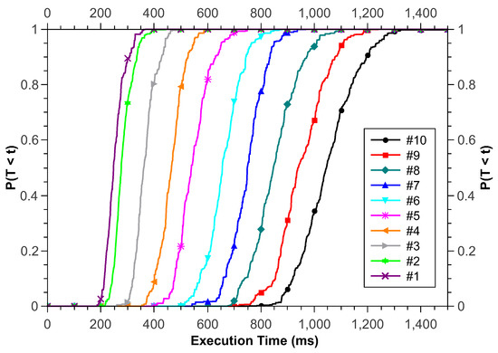
Figure 10.
Cumulative Distribution Functions for Study 2.
4.2.3. Model Validation
The validation of the proposed system SPN model is detailed in this section. We performed different experiments in practical scenarios to measure the system’s MRT and then compare with the MRT computed by the proposed model for the sake of validation. An experimental laboratory test-bed (as shown in Figure 11) was developed to help validate the analysis results of the proposed model, which has the following configuration, (i) internet bandwidth at 40 Mbps, (ii) a computer for synthetic request generation with CPU of Intel Core i7 2.4 Ghz and RAM of 8 GB capacity.
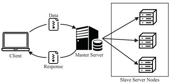
Figure 11.
Validation Test-Bed Architecture (adapted from [35]).
We adopted a well-known word processing algorithm (Word Count Algorithm https://tinyurl.com/y8hofs5x, accessed on 10 November 2020) using MapReduce for big data processing. The algorithm can help compute the number of keywords in a text file upon their unique occurrences. The texts in the file are split into data blocks. The number of splits determines the number of mapping steps for split jobs. Afterwards, all split tasks are allocated and distributed to slave nodes. This process generates key-value pairs in which a key is mapped to a specific word while the key’s value is exactly the number 1. It is worth noting that, the mapping results do not imply the accumulated occurrences of words in a text file. The sorting process generates a list of all values by key, after that, the reducing process summarizes the occurrences of each key in the list to obtain the total number of each keywords. Finally, the reducing process creates a file consisting of the number of occurrences in the text file for each word. In experimental implementation, the execution of the mapping and reducing processes is allocated to each node. At the end, the processing time of a text file at 15 MB size is measured on a single node, and the measured output is used to feed to model parameters.
We deployed the edge into four different machines—one master and three other slave nodes. The arrival rate of a new request is set to the value 230 s. Each request is to process three consecutive text files at 40 MB in size each. To comply with Little’s law, the processing tasks are allocated to machines in the way that each machine processes only one file at a time. In this way, the experiment can obtain the highest level of parallelism without stressing the computer system. The mean processing time of one file on a slave node (PD) is necessarily measured in order to feed to parameters in the proposed model. The values of parameters in the SPN model used for model validation are summarized as follows, (i) PD: 51.7 s, (ii) AD: 230 s, (iii) MC: 20 and (iv) SC: 3. Using stationary analysis for the SPN model, the calculated value of MRT was 86.74 s. Furthermore, the value of total resource utilization was 22.4%.
The experiment is conducted by repeatedly dispatching a specific number of consecutive requests (100 requests) to the edge. The extracted sample showed a normal distribution with a mean of 86.906 s. The One-Sample t-Test (One Sample t-Test https://tinyurl.com/yanthw4e, accessed on 20 November 2020) is used to make inferences about a population mean, based on data from a random sample. One-Sample t-Test is adopted to compare the values of MRT which are generated by the model and by the sample mean, respectively. It should be pointed out that, the case which both means are equal falls in the null hypothesis. The test results are (i) mean: 86.91 s, (ii) standard deviation: 5.039, (iii) standard error mean: 0.504, (iv) 95% confidence interval: (85.906, 87.905), (v) T: 0.41, (vi) p-value: 0.684.
As per observed, it is not possible to disprove the null hypothesis with 95% confidence due to the reason that the p-value is bigger than the number 0.05, according to statistics. As per examined, we noticed a statistical equivalence between the generated results of the proposed SPN model and the measured results of test-bed experiments. At this level, the proposed model is practically appropriate for expansion in performance evaluation of real-world big-scale edge computing infrastructures. The proposed model literally represents an actual environment and computing system, and thus, it can be used for planning and assessment in the development of MEC infrastructures.
5. Evaluation of MEC Availability
This section presents two SPN models focusing on the availability evaluation of the MEC architecture previously presented. First, we present a base proposal, and next, an extended version is detailed.
5.1. Base Proposal—Architecture
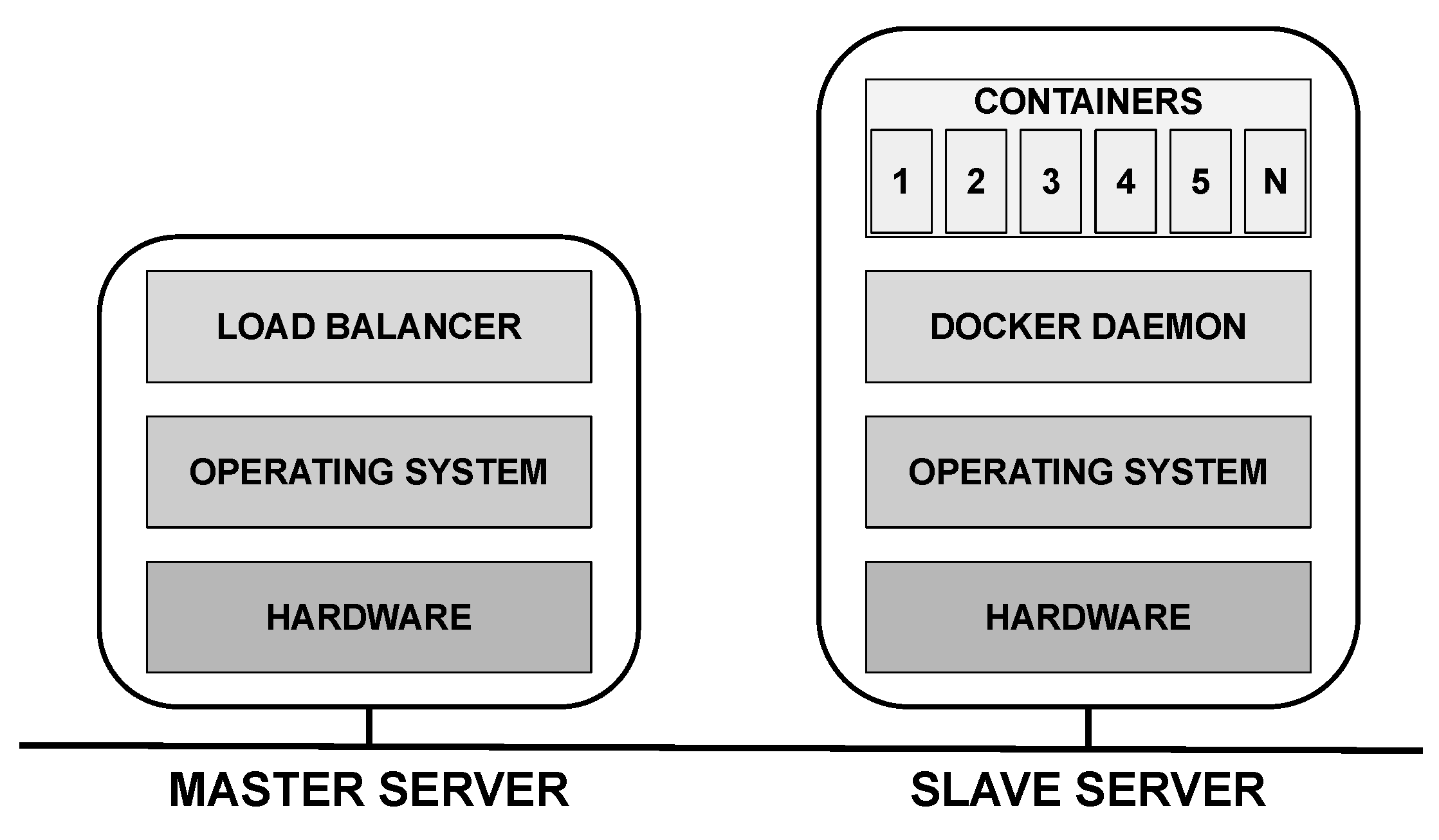
Figure 12 shows the layered architecture assigned to the two servers. The master server is responsible for receiving requests from mobile devices and distributing them to slave nodes, so the software component called load balancer is responsible for such distribution. The distribution policy must be defined by the evaluator. The slave server runs a virtualization platform, which we illustrate as being the Docker (Docker: https://www.docker.com/products/, accessed on 25 October 2020), above which are the N containers.The model user may adopt any virtualization platform. In this case, the user should consider the respective MTTF/MTTR to feed the model.
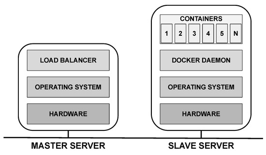
Figure 12.
Layered architecture composed of two servers.
Base Proposal—SPN Model
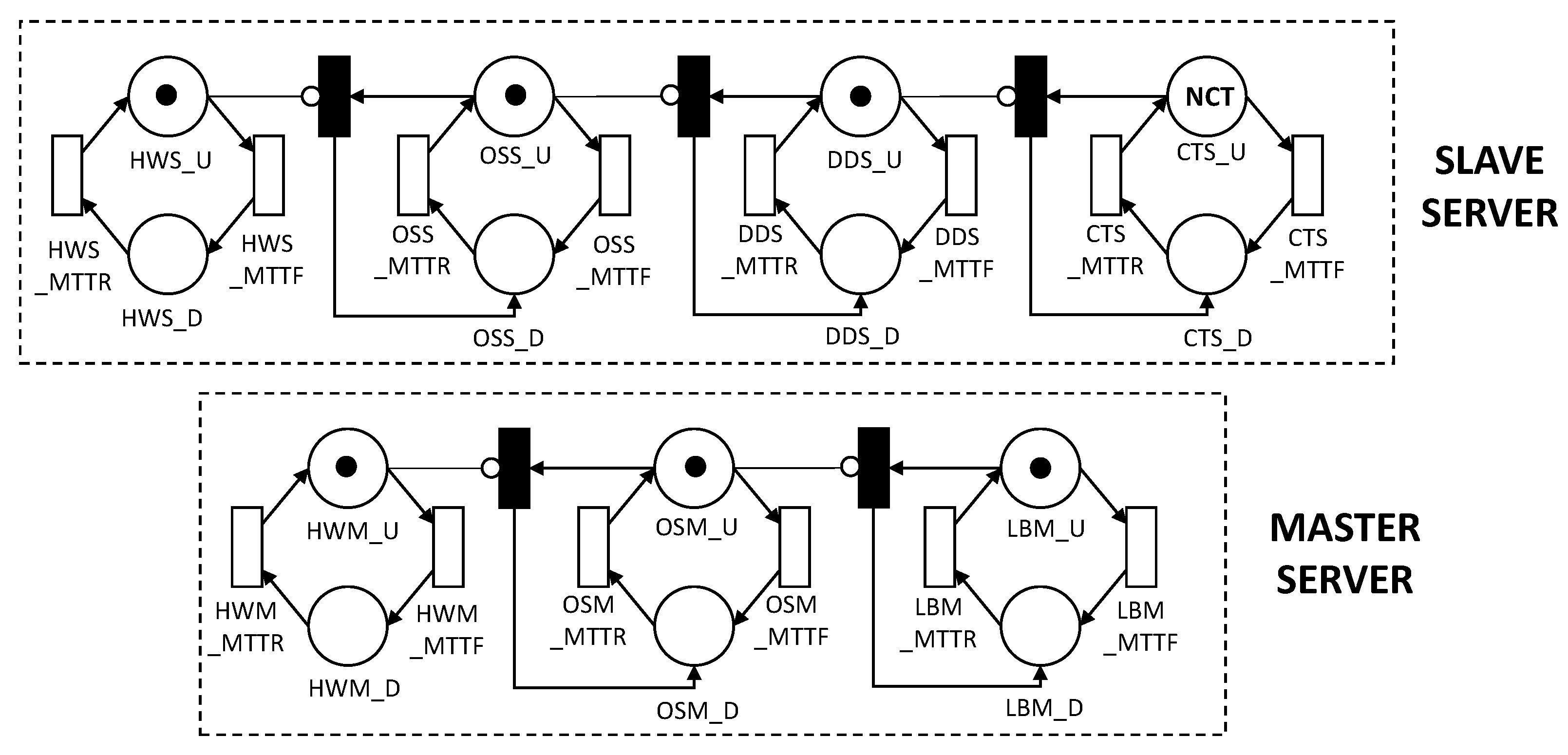
Figure 13 presents an SPN model for the MEC architecture with the following functions: (i) Master Server is responsible for receiving requests from mobile devices and distributing them among slave server nodes; (ii) Slave Server is responsible for processing the data received from the master server. The components in the model correspond to the same layers presented in Figure 12. Each component has its respective MTTF and MTTR. Both master server and slave server were modeled, taking into account the dependency between the components; that is when a component fails the immediate transitions will trigger the next dependent components to fail as well.

Figure 13.
SPN base model for an MEC architecture with master–slave layout.
The NCT marking corresponds to the number of available containers. The slave server will be working when it has NCT tokens in the place CTS_U (active container). The evaluator can define in the metric (with such NCT mark) how many containers must be active for the system to be working. We consider that slave server is not working when it has a token in one of the following locations: HWS_D (hardware down), OSS_D (operating system down), DDS_D (docker daemon down), CTS_D (container down). Changing between active and inactive state is caused by the following transitions: HWS_MTTF, OSS_MTTF, DDS_MTTF and CTS_MTTF—for time medium to failure—and HWS_MTTR, OSS_MTTR, DDS_MTTR, and CTS_MTTR—for average time to repair.
The Master Server will be running when it has tokens in the LBM_U location (load balancer active). We consider that Master Server is not working when it has a token in one of the following locations: HWM_D (hardware down), OSM_D (operating system down), LBM_D (load balancer down). The change between the active and inactive state is caused by the transitions: HWM_MTTF, OSM_MTTF, and LBM_MTTF—for mean time to failure—and HWM_MTTR, OSM_MTTR, and LBM_MTTR—for mean time to repair.
Two metrics were applied: availability and downtime. The availability equation represents the sum of probabilities of components in the upstate. P stands for probability, and # stands for the number of tokens in a given location. The downtime (D) can be obtained by , where A represents the availability of the system, and 8760 represents the number of hours in the year. For the availability, the system is fully functional when all containers and the LB (load balancer) are both active. Therefore, the availability is calculated by: .
Guard conditions ensure that transitions are only triggered when a specific condition is satisfied. The guard condition ensures that the model reflects the behaviors of the system in the real world. For example, the transition OSS_MTTR has the following guard condition: , meaning that to trigger the recovery transition from the operating system, the hardware (HW) must be active. Following this example, the transitions DDS_MTTR, CTS_MTTR, OSM_MTTR, and LBM_MTTR follow the same pattern and are only activated if their respective dependency components are active. See Table 5 for more details.

Table 5.
Guard conditions used to guarantee components dependency.
5.2. Extended Proposal—Architecture
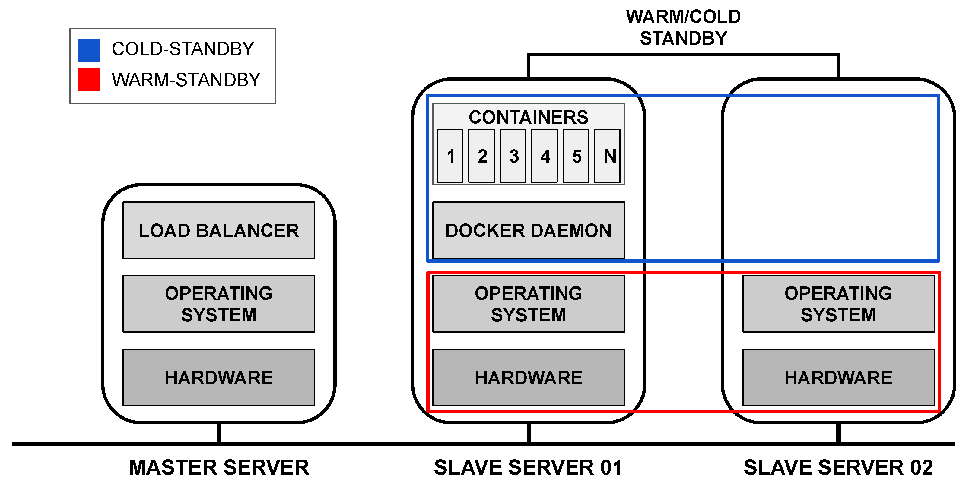
A significant limitation of the base proposal is that if one of the two servers fail, the entire system will stop working. For this reason, Figure 14 presents a second proposal for redundant architecture, which aims to improve the system’s availability rate compared to the base architecture. For this architecture, we consider redundancy only on the slave server to assess a possible availability improvement where data processing happens. Such a redundancy decision is based on the sensitivity analysis that will be presented in Section 5.3.2. The sensitivity analysis evidenced the containers as the most critical components in the system. Both slave servers are always working; however, Docker and the containers on the slave server 02 are instantiated only if the slave server 01 fails. Therefore, there is a redundancy mechanism of warm standby [41] in the hardware and operating system, and cold standby [42] in the Docker and containers.
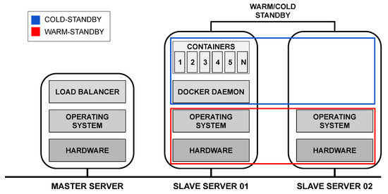
Figure 14.
Layered architecture with redundancy under the slave server.
Extended Proposal—SPN Model
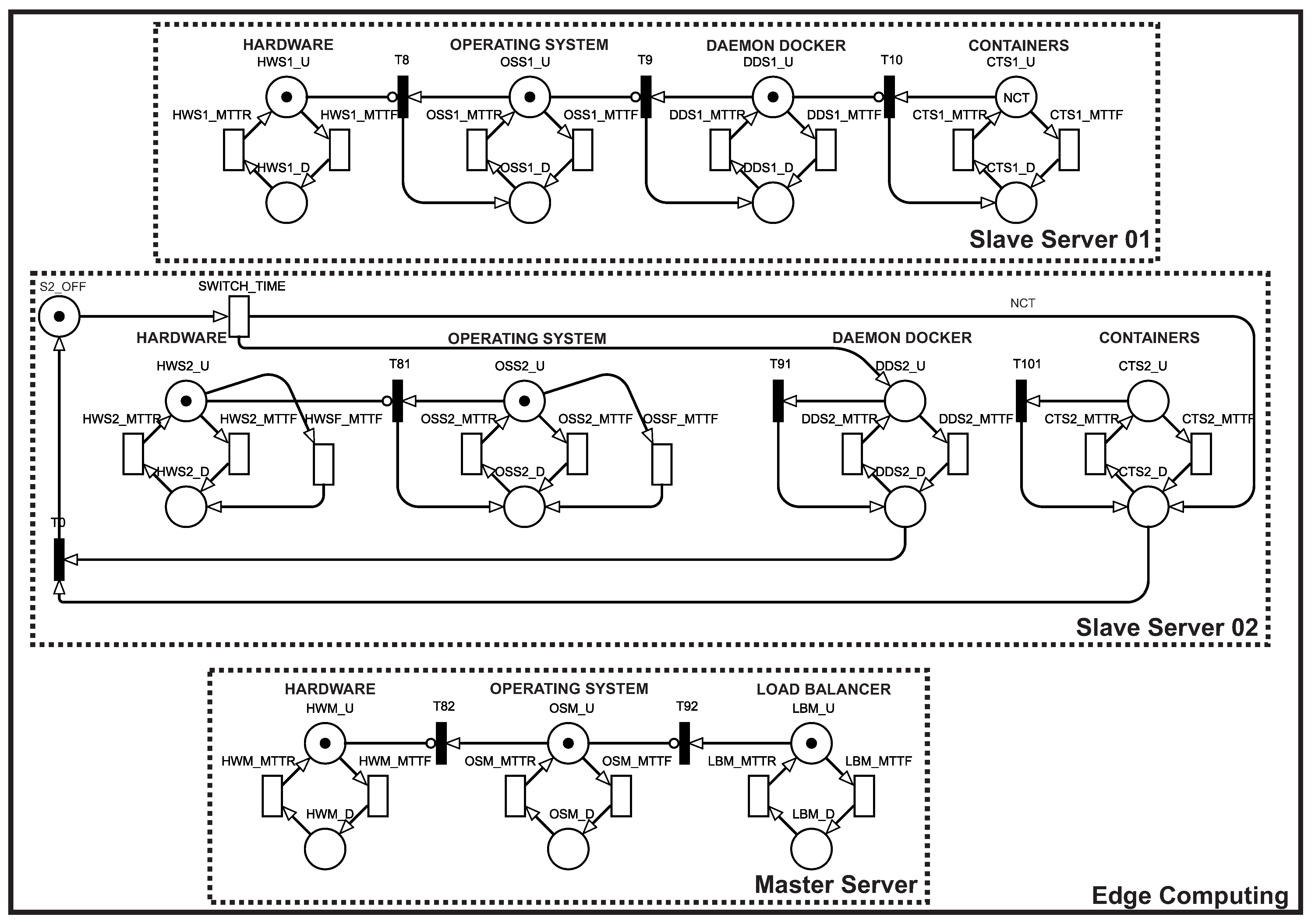
Figure 15 presents an extended SPN model for the MEC architecture, with 2 slave servers and a master server. The extended SPN model presents a change in the slave server, while the master server maintains the same components. As mentioned earlier, this new model features a hybrid mechanism between warm-standby (HW and OS components) and cold-standby (DD and CTS components). If any of the software components of slave server 01 fail, other components will be started in slave server 02. Two new transitions were added to satisfy these conditions, HWSF_MTTF and OSSF_MTTF (in the slave server 02 block), which represent the MTTF for HW and OS when Docker is down, that is, HW and OS are idle.
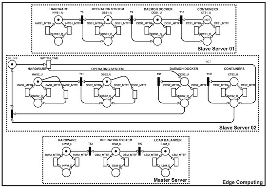
Figure 15.
Extended SPN model for an MEC architecture with redundant slave server.
It is enough to observe the state of the upper layers of the architecture to calculate availability due to components dependency. Thus, the system will be working when both containers and the load balancer are working. The NCT is the parameter that represents the maximum number of containers that the system can run. In other words, the sum of the number of active containers on the two redundant servers cannot exceed the value of NCT. The SWITCH_TIME transition is triggered when the slave server 01 fails, and this time corresponds to the time it takes for the slave server 02 Docker to start up. Firing SWITCH_TIME also puts the number of containers corresponding to NCT in place CTS2_D, that is, the containers are created with inactive status on the slave server 02, and they will take some time to be instantiated, corresponding to transition CTS2_MTTR. Therefore, the availability of the second model is given by . It is worth mentioning that the MTTF transitions are infinite server type (parallel), and the MTTR transitions are single server type (concurrent).
Table 6 shows the guard conditions used for the operation of the system in the extended model. In this case, using guard conditions avoids visual pollution in the model since several connections should be made, and this would make the model difficult to understand.

Table 6.
Guard conditions to the extended model.
5.3. Case Studies
This section presents a case study with an availability assessment and a sensitivity analysis, considering the two presented models. Some input parameters are required to perform the evaluation. The MTTF and MTTR values for each component were extracted from [43,44]. Table 7 shows the input values of the model components. As much as the proposed model supports different configurations for each server, in terms of simplification, we have chosen to use the same configuration between the three servers. The time to activate the redundant server in the transition SWITCH_TIME is 0.0833333 h, extracted from [43].

Table 7.
Extended model input values.
5.3.1. Availability Analysis
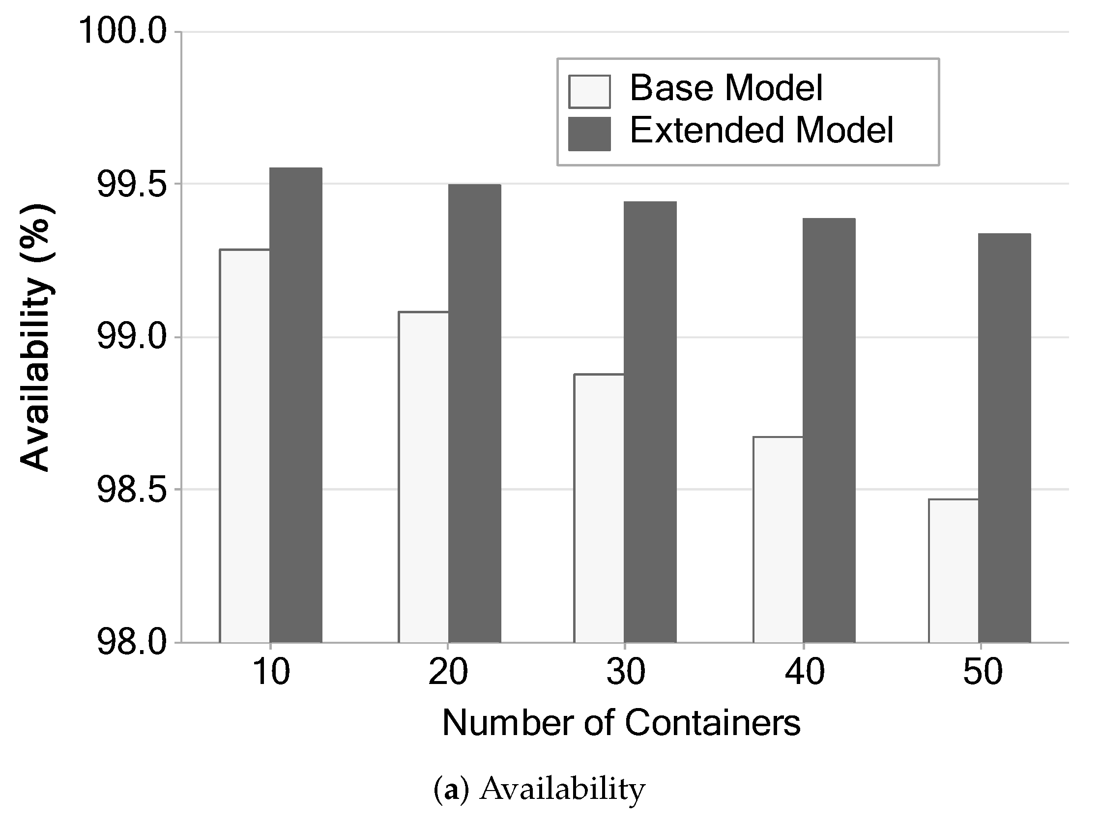
This section presents the availability analysis. Five scenarios were defined, varying the number of available containers (10, 20, 30, 40, and 50 containers). These scenarios were generated in order to compare the availability of the two models as well as the impact that the number of containers generates in each architecture.
Figure 16 shows availability and downtime calculated by stationary analysis with the Mercury [45] tool. The availability variation shown in Figure 16a shows that availability drops as new containers are instantiated. In addition, the availability of the extended model tends to fall more slowly than in the base model. We believe that this fact occurs due to the redundancy implemented in the extended model. Even if we add containers, there will be a redundant component to supply the eventual failures in the slave server 01.
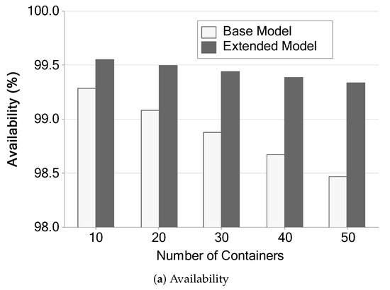
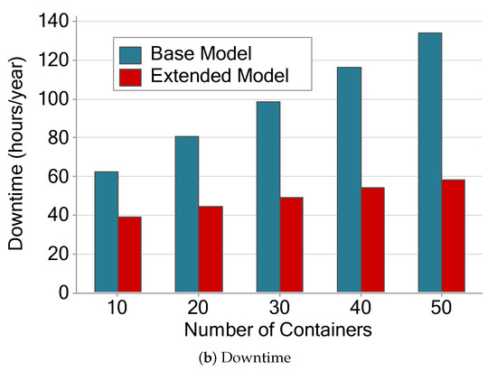
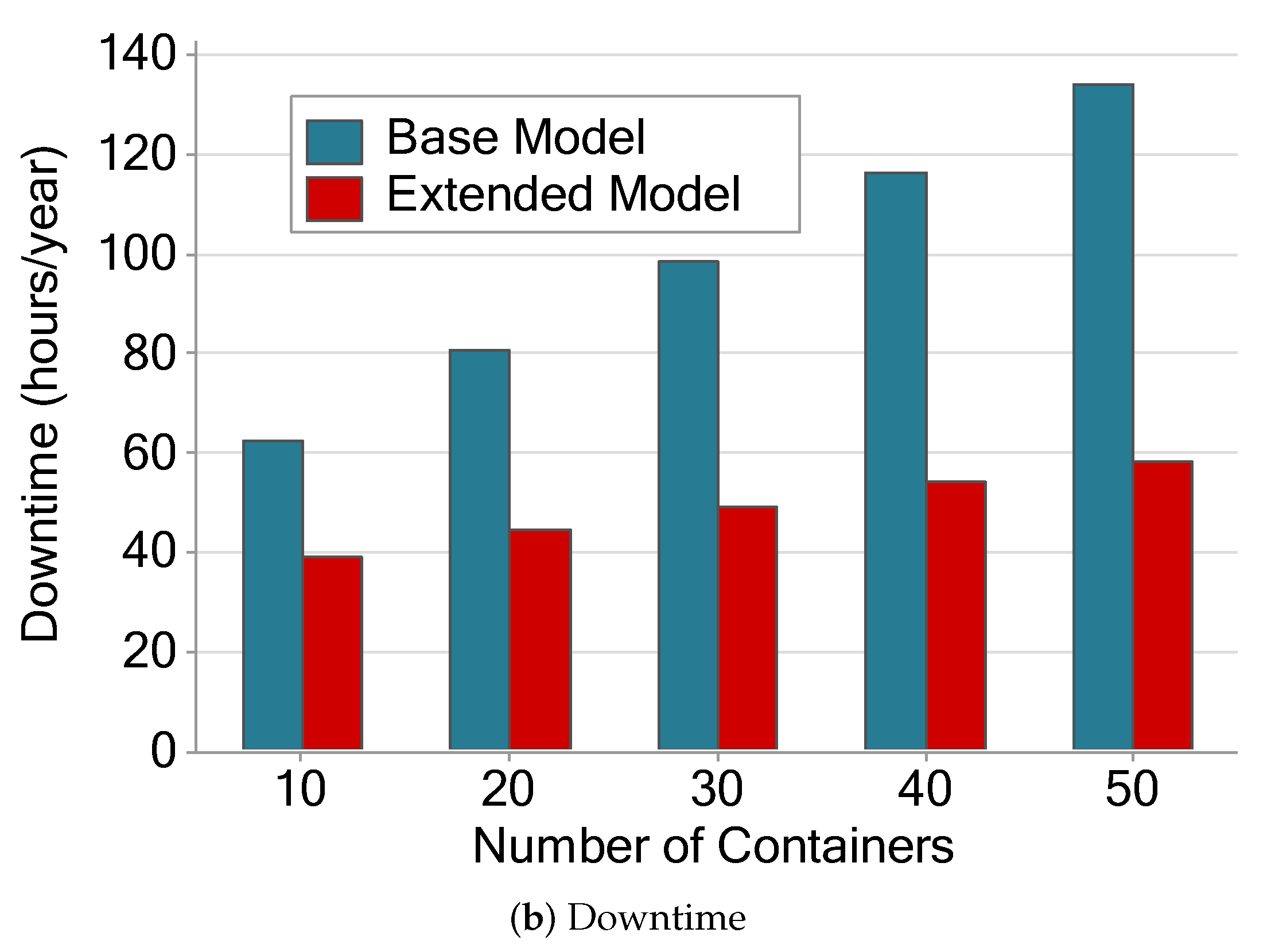
Figure 16.
Availability and downtime of the two architectures varying the number of containers.
Figure 16b shows downtime in hours per year. The extended model downtime tends to be much shorter than the base model. The base model ranges from 60 to 130 h/y. The extended model ranges from 40 to 60 h/y. The extended model’s downtime remains below the base model even with five times more containers. The individual values of the base model grow noticeably more, and from the third scenario, they become twice as long as the extended model. After the fourth scenario, the time passes 100 h/y, while the extended model remained below sixty in all scenarios.
These results are expected since the more components we have in a system, the higher the chances of one of them failing, and the more they fail, the more time it takes to repair. Our metric considers the system working when all containers are up; therefore, higher failure rates will negatively impact the availability. This behavior is observed even in the extended model. However, in the extended model, it happens in a much more subtle way, because there is a redundancy mechanism in the server.
5.3.2. Transition Sensitivity Analysis
For the sensitivity analysis, the MTTF and MTTR parameters were varied by five values within a range defined by the maximum and minimum values (50% plus and minus the default value). Table 8 presents the components and their respective sensitivity indices that cause significant impacts on the availability of the system. The most significant components will be exposed and discussed below.

Table 8.
Values resulting from the sensitivity analysis on the timed transitions of the SPN models.
The failure and recovery times of the containers were the components that most impacted the availability of the base model; this can also be seen by looking at Figure 16a, so we can consider the containers as essential components of the system. Data are processed in the containers. The longer they stay out of operation, the more impaired is the efficiency of the system. Right after that are the failure times of slave server components (OS, DD, and HW). As these components are parts that “support” the containers, their uptime has a significant impact on the uptime of the containers. The operating times of master server components come subsequently. If the master server fails, no data will arrive to be processed on any slave server.
As aforementioned, the sensitivity analysis results in the base model were considered to generate an extended model. In the extended model, there was an inversion of indexes order regarding the component’s relevance. By adding the hybrid redundancy strategy, the sensitivity index of the slave server can be significantly reduced. Given the redundancy, when any component of slave server 01 fails, slave server 02 will be activated. The components of the master server ended up becoming more relevant as they did not have a redundancy mechanism. The indexes were equal to the first analysis in the base model. Right after that, we have SWITCH_TIME, which is essential for defining the time it takes to initialize slave server 02, becoming a relevant variable. The less relevant transitions were those related to failure of hardware (HWSF_MTTF) and operating system (OSSF_MTTF) in idle state. These transitions have very high values. Other components will fail many times before reaching that time.
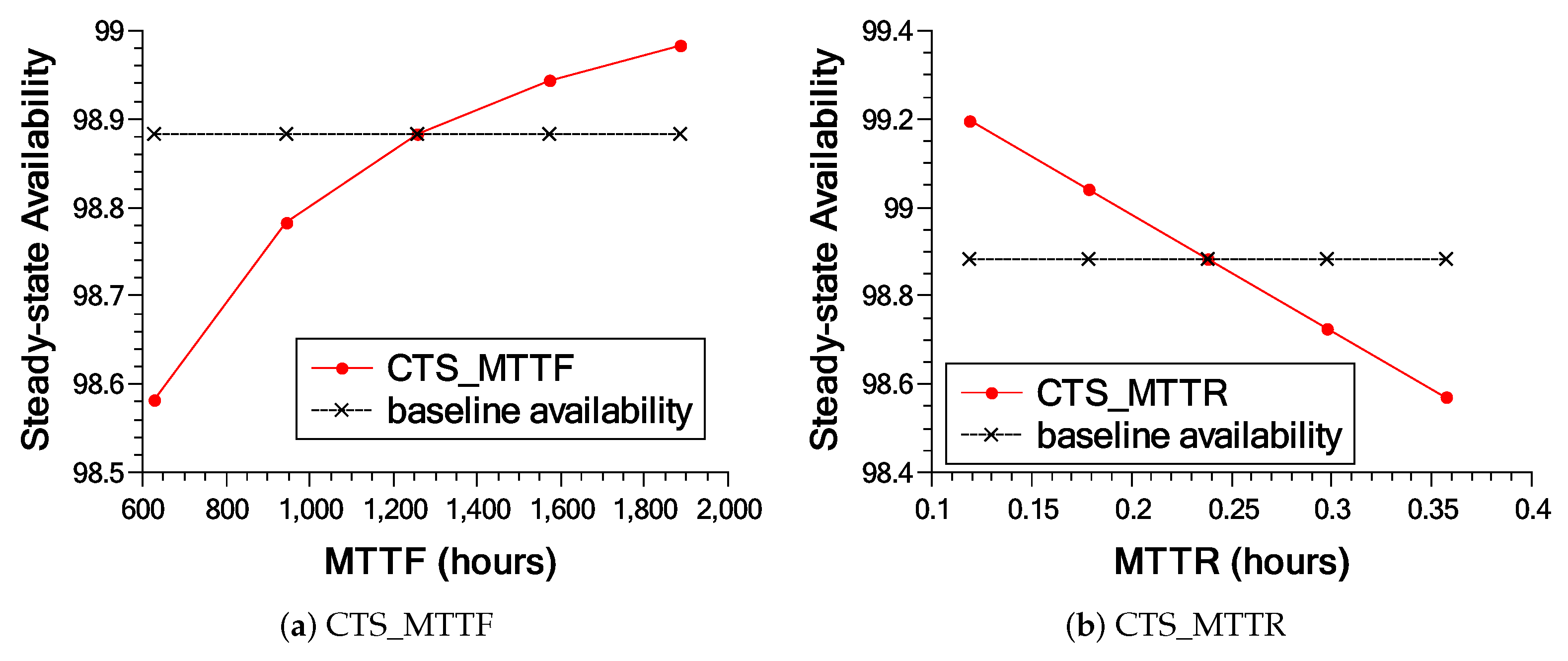
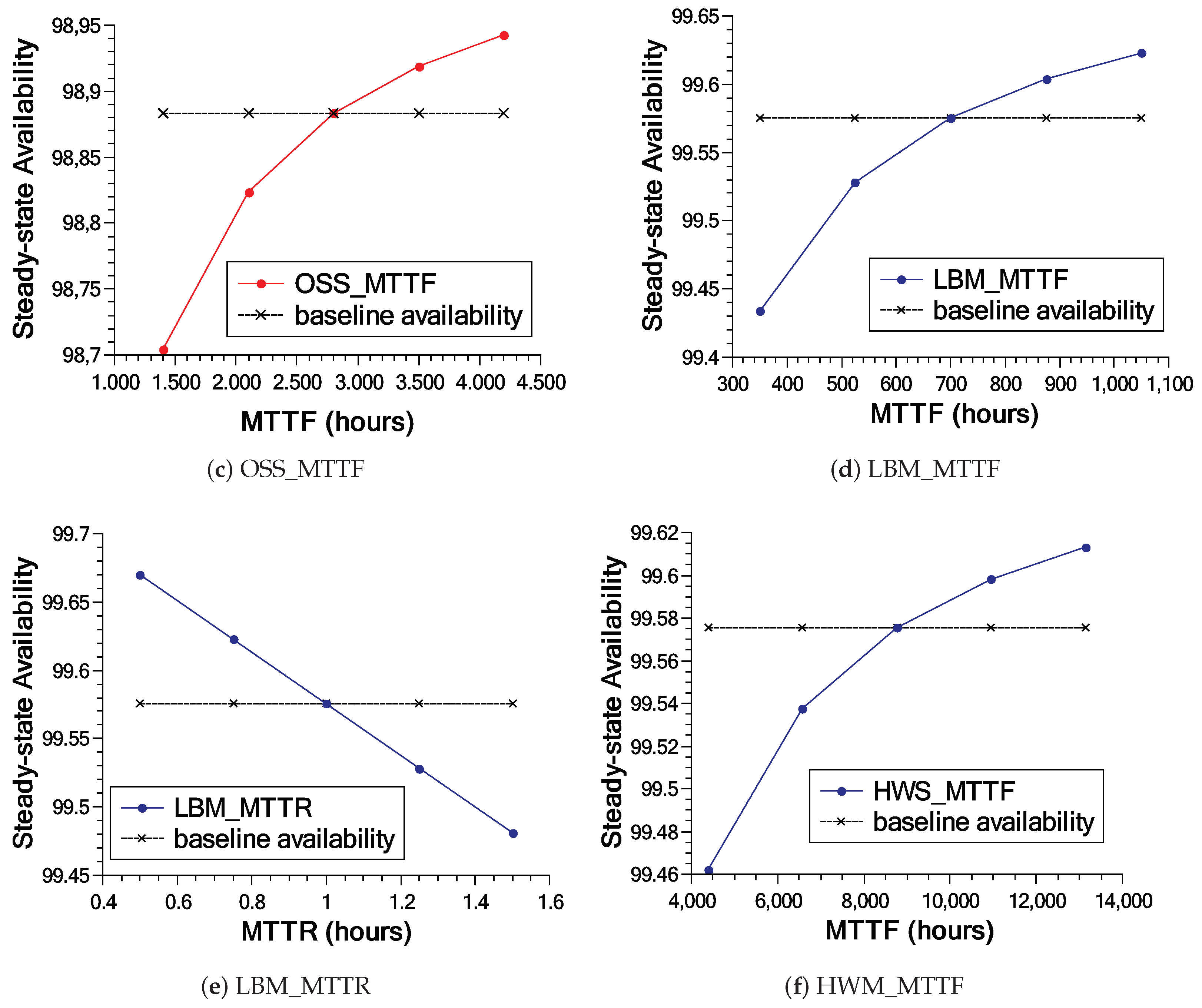
Figure 17 shows in more detail the impact of the three most essential components of each model. As can be seen in Figure 17a–c, varying the parameters influences availability up to a certain point. All base model results are below 99% availability, with the exception of the CTS_MTTR transition (Figure 17b). The results of the extended model present much higher values compared to the base model (see Figure 17d–f). The results of the extended model, different from the base model, always remain above 99%, since it presents redundancy in the components that were impacting availability in the base model.
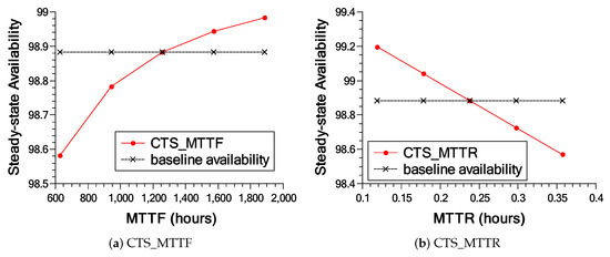
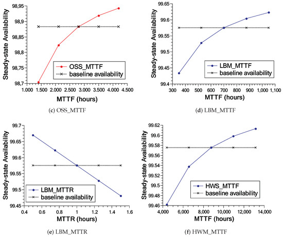
Figure 17.
Results (a–c) show the three most important transitions in the base model; Results (d–f) present the results of the sensitivity analysis of the most important transitions in the extended model.
5.4. Discussions
Performance Evaluation: To comprehensively assess the performance of the underlying MEC architecture, we proposed an SPN model which allows estimating MRT and the level of resource utilization at the edge of the network. Ones may configure up to 5 input parameters, which allows a high level of evaluation flexibility. A numerical analysis was performed using real data from a reference paper to feed parameters in the proposed model. The numerical analysis helps investigate the behavior of four metrics (MRT, discard rate, master node utilization, and slave nodes utilization) as a function of the arrival delay. As per observed, the arrival delay is the parameter that exposes a clearly significant impact on the system’s performance compared to the remaining parameters.
A refined model with an absorbing state was developed to explore when applications are most likely to complete their execution through the use of CDF. Two case-studies were conducted to demonstrate the use of this model. In the first case-study, a verification was performed to see which configuration of a slave server best meets the requirements of an infrastructure administrator, according to the total time desired for the application execution. The finding of this case-study is that the total time for execution increases as resources decrease. In the second case-study, we observed the probability of execution based on the time between arrivals. We found that as the time between arrivals increases, the total time required to complete application execution also grows. The performance model was validated with a real experiment, the results of which indicated equality between experiment and model with p-value equal to 0.684 by t-Test.
Availability Assessment: An SPN model was also developed to represent and evaluate the availability of an underlying MEC architecture. It is feasible to analyze which were the most important components of the system based on the proposed model. Furthermore, thus, it is also possible to propose an extensional architecture focusing on these components. Scenarios with different quantities of containers were analyzed. As per investigated, the extended architecture shows a considerable improvement in availability compared to the base architecture. The containers were exposed to be the significantly important components in both models, and that a server with distributed responsibility is not always the bottleneck of the system. The results of the extended model, different from the base model, always remain above 99%, since it presents redundancy in the components that were impacting availability in the base model.
Future Extensions: Regarding the performance evaluation, we intend to perform other numerical analyzes, adding more servers or considering different types of applications. We also intend to extend the proposed model to measure energy expenditure and explore allocation between multiple MEC towers. On the other hand, the availability model can be extended by taking into account redundancy of the components in the master server, and the consideration of different operational scenarios for testing the models is also an essential extension.
6. Conclusions and Future Works
In this paper, we proposed (i) an original performance SPN model, (ii) its refined model with an absorbing state and (iii) an availability SPN model, for performance and availability assessment of an MEC infrastructure. Comprehensive analyses were performed to assimilate different aspects of the system operations in terms of performance and availability. Performance metrics were analyzed in the original performance model including MRT, discard rate, and utilization of master and slave nodes with regard to arrival delay. Two case-studies using the refined model with an absorbing state were conducted to investigate the completion time of application execution. An availability model was first introduced for a base-line MEC with the basic configuration of a master and a slave node, while an extensional one was proposed when redundancy of slave nodes was taken into account. Availability metrics were analyzed including operational availability and downtime hours in a year. Availability sensitivity wrt. MTTFs and MTTRs were performed in a comprehensive manner. The analysis results pinpoint essential system parameters which incur significant impacts on performance and availability of an MEC. As a result, this study helps comprehend operational characteristics of an MEC regarding performance and availability metrics, and thus helps design actual MEC architectures and plan in advance economic operations of practical MEC systems.
Author Contributions
Conceptualization, F.A.S.; methodology, F.A.S.; software, C.B., L.R., and B.S.; validation, F.A.S. and I.F.; formal analysis, C.B., L.R., B.S. and I.F.; investigation, F.A.S. and T.-A.N.; resources, F.A.S. and T.-A.N.; data curation, C.B., L.R., and B.S.; writing—original draft preparation, C.B., L.R., and B.S.; writing—review and editing, T.-A.N., D.M., J.-W.L. and F.A.S.; visualization, C.B., L.R., and B.S.; supervision, D.M., J.-W.L. and F.A.S.; project administration, F.A.S. and T.-A.N.; funding acquisition, D.M. and J.-W.L. All authors have read and agreed to the published version of the manuscript.
Funding
This research was partially funded by the National Council for Scientific and Technological Development—CNPq, Brazil, through the Universal call for tenders (Process 431715/2018-1). This research was supported by Basic Science Research Program through the National Research Foundation of Korea (NRF) funded by the Ministry of Education (No. 2020R1A6A1A03046811). This research was supported by the MSIT (Ministry of Science and ICT), Korea, under the ITRC(Information Technology Research Center) support program (IITP-2020-2016-0-00465) supervised by the IITP (Institute for Information & Communications Technology Planning & Evaluation) This research was funded and conducted under "The Competency Development Program for Industry Specialist" of the Korean Ministry of Trade, Industry and Energy (MOTIE), operated by Korea Institute for Advancement of Technology (KIAT). (No. N0002428).
Acknowledgments
The authors would like to thank anonymous reviewers for their constructive comments and suggestions.
Conflicts of Interest
The authors declare no conflict of interest.
References
- Statista Forecast. Available online: https://www.statista.com/statistics/245501/multiple-mobile-device-ownership-worldwide/ (accessed on 14 February 2020).
- Orsini, G.; Bade, D.; Lamersdorf, W. Computing at the mobile edge: Designing elastic android applications for computation offloading. In Proceedings of the 2015 8th IFIP Wireless and Mobile Networking Conference (WMNC), Munich, Germany, 5–7 October 2015; pp. 112–119. [Google Scholar]
- Borgia, E.; Bruno, R.; Conti, M.; Mascitti, D.; Passarella, A. Mobile edge clouds for Information-Centric IoT services. In Proceedings of the 2016 IEEE symposium on computers and communication (ISCC), Messina, Italy, 27–30 June2016; pp. 422–428. [Google Scholar]
- Kertesz, A.; Pflanzner, T.; Gyimothy, T. A Mobile IoT Device Simulator for IoT-Fog-Cloud Systems. J. Grid Comput. 2019, 17, 529–551. [Google Scholar] [CrossRef]
- Marotta, M.A.; Faganello, L.R.; Schimuneck, M.A.K.; Granville, L.Z.; Rochol, J.; Both, C.B. Managing mobile cloud computing considering objective and subjective perspectives. Comput. Netw. 2015, 93, 531–542. [Google Scholar] [CrossRef]
- Othman, M.; Khan, A.N.; Abid, S.A.; Madani, S.A. MobiByte: An application development model for mobile cloud computing. J. Grid Comput. 2015, 13, 605–628. [Google Scholar]
- Vaquero, L.M.; Rodero-Merino, L.; Caceres, J.; Lindner, M. A break in the clouds: Towards a cloud definition. ACM Sigcomm Comput. Commun. Rev. 2008, 39, 50–55. [Google Scholar] [CrossRef]
- Dinh, H.T.; Lee, C.; Niyato, D.; Wang, P. A survey of mobile cloud computing: Architecture, applications, and approaches. Wirel. Commun. Mob. Comput. 2013, 13, 1587–1611. [Google Scholar] [CrossRef]
- Jararweh, Y.; Doulat, A.; AlQudah, O.; Ahmed, E.; Al-Ayyoub, M.; Benkhelifa, E. The future of mobile cloud computing: Integrating cloudlets and mobile edge computing. In Proceedings of the 2016 23rd International conference on telecommunications (ICT), Thessaloniki, Greece, 16–18 May 2016; pp. 1–5. [Google Scholar]
- Jararweh, Y.; Doulat, A.; Darabseh, A.; Alsmirat, M.; Al-Ayyoub, M.; Benkhelifa, E. SDMEC: Software defined system for mobile edge computing. In Proceedings of the 2016 IEEE International Conference on Cloud Engineering Workshop (IC2EW), Berlin, Germany, 4–8 April 2016; pp. 88–93. [Google Scholar]
- Ahmed, A.; Ahmed, E. A Survey on Mobile Edge Computing. In Proceedings of the Australia’s National Linux Conference, Geelong, Australia, 1–5 February 2016. [Google Scholar] [CrossRef]
- Marsan, A. Modelling with Generalized Stochastic Petri Nets; Wiley Series in Parallel Computing; Wiley: Hoboken, NJ, USA, 1995. [Google Scholar]
- Trivedi, K. Probability and Statistics with Reliability, Queueing, and Computer Science Applications, 2nd ed.; Wiley Interscience Publication: Hoboken, NJ, USA, 2002. [Google Scholar]
- Silva, F.A.; Rodrigues, M.; Maciel, P.; Kosta, S.; Mei, A. Planning mobile cloud infrastructures using stochastic petri nets and graphic processing units. In Proceedings of the 2015 IEEE 7th International Conference on Cloud Computing Technology and Science (CloudCom), Vancouver, BC, Canada, 30 November–3 December 2015; pp. 471–474. [Google Scholar]
- Santos, G.L.; Gomes, D.; Kelner, J.; Sadok, D.; Silva, F.A.; Endo, P.T.; Lynn, T. The internet of things for healthcare: Optimising e-health system availability in the fog and cloud. Int. J. Comput. Sci. Eng. 2020, 21, 615–628. [Google Scholar] [CrossRef]
- Ferreira, L.; da Silva Rocha, E.; Monteiro, K.H.C.; Santos, G.L.; Silva, F.A.; Kelner, J.; Sadok, D.; Bastos Filho, C.J.; Rosati, P.; Lynn, T.; et al. Optimizing Resource Availability in Composable Data Center Infrastructures. In Proceedings of the 2019 9th Latin-American Symposium on Dependable Computing (LADC), Natal, Brazil, 19–21 November 2019; pp. 1–10. [Google Scholar]
- Silva, F.A.; Kosta, S.; Rodrigues, M.; Oliveira, D.; Maciel, T.; Mei, A.; Maciel, P. Mobile cloud performance evaluation using stochastic models. IEEE Trans. Mob. Comput. 2018, 17, 1134–1147. [Google Scholar] [CrossRef]
- da Silva Pinheiro, T.F.; Silva, F.A.; Fé, I.; Kosta, S.; Maciel, P. Performance prediction for supporting mobile applications’ offloading. J. Supercomput. 2018, 74, 4060–4103. [Google Scholar] [CrossRef]
- Pinheiro, T.; Silva, F.A.; Fe, I.; Kosta, S.; Maciel, P. Performance and Data Traffic Analysis of Mobile Cloud Environments. In Proceedings of the 2018 IEEE International Conference on Systems, Man, and Cybernetics (SMC), Miyazaki, Japan, 7–10 October 2018; pp. 4100–4105. [Google Scholar]
- Zhang Ke, M.Y.; Leng, Z.Q.; Li, P.X. Energy-efficient offloading for mobile edge computing in 5G heterogeneous networks. IEEE Access 2016, 4, 5896–5907. [Google Scholar] [CrossRef]
- Trinh, C.; Yao, L. Energy-aware mobile edge computing for low-latency visual data processing. In Proceedings of the 2017 IEEE 5th International Conference on Future Internet of Things and Cloud (FiCloud), Prague, Czech Republic, 21–23 August 2017; pp. 128–133. [Google Scholar]
- Mao, Y.; Zhang, J.; Letaief, K.B. Dynamic computation offloading for mobile-edge computing with energy harvesting devices. IEEE J. Sel. Areas Commun. 2016, 34, 3590–3605. [Google Scholar] [CrossRef]
- Badri, H.; Bahreini, T.; Grosu, D.; Yang, K. Multi-stage stochastic programming for service placement in edge computing systems: Poster. In Proceedings of the Second ACM/IEEE Symposium on Edge Computing, San Jose, CA, USA, 12–14 October 2017; p. 28. [Google Scholar]
- Zakarya, M.; Gillam, L.; Ali, H.; Rahman, I.; Salah, K.; Khan, R.; Rana, O.; Buyya, R. Epcaware: A game-based, energy, performance and cost efficient resource management technique for multi-access edge computing. IEEE Trans. Serv. Comput. 2020. [Google Scholar] [CrossRef]
- Guillén, M.A.; Llanes, A.; Imbernón, B.; Martínez-España, R.; Bueno-Crespo, A.; Cano, J.C.; Cecilia, J.M. Performance evaluation of edge-computing platforms for the prediction of low temperatures in agriculture using deep learning. J. Supercomput. 2021, 77, 818–840. [Google Scholar] [CrossRef]
- Costa, I.; Araujo, J.; Dantas, J.; Campos, E.; Silva, F.A.; Maciel, P. Availability Evaluation and Sensitivity Analysis of a Mobile Backend-as-a-service Platform. Qual. Reliab. Eng. Int. 2016, 32, 2191–2205. [Google Scholar] [CrossRef]
- Matos, R.; Araujo, J.; Oliveira, D.; Maciel, P.; Trivedi, K. Sensitivity analysis of a hierarchical model of mobile cloud computing. Simul. Model. Pract. Theory 2015, 50, 151–164. [Google Scholar] [CrossRef]
- Dantas, J.; Matos, R.; Araujo, J.; Maciel, P. Models for dependability analysis of cloud computing architectures for eucalyptus platform. Int. Trans. Syst. Sci. Appl. 2012, 8, 13–25. [Google Scholar]
- Araujo, J.; Silva, B.; Oliveira, D.; Maciel, P. Dependability evaluation of a mhealth system using a mobile cloud infrastructure. In Proceedings of the 2014 IEEE International Conference on Systems, Man, and Cybernetics (SMC), San Diego, CA, USA, 5–8 October 2014; pp. 1348–1353. [Google Scholar]
- Oliveira, D.; Araujo, J.; Matos, R.; Maciel, P. Availability and energy consumption analysis of mobile cloud environments. In Proceedings of the 2013 IEEE International Conference on Systems, Man, and Cybernetics, Manchester, UK, 13–16 October 2013; pp. 4086–4091. [Google Scholar]
- Santos, G.L.; Endo, P.T.; da Silva Lisboa, M.F.F.; da Silva, L.G.F.; Sadok, D.; Kelner, J.; Lynn, T. Analyzing the availability and performance of an e-health system integrated with edge, fog and cloud infrastructures. J. Cloud Comput. 2018, 7, 16. [Google Scholar] [CrossRef]
- Yin, X.; Cheng, B.; Wang, M.; Chen, J. Availability-aware Service Function Chain Placement in Mobile Edge Computing. In Proceedings of the 2020 IEEE World Congress on Services (SERVICES), Beijing, China, 18–23 October 2020; pp. 69–74. [Google Scholar]
- Li, Y.; Wang, S. An Energy-Aware Edge Server Placement Algorithm in Mobile Edge Computing. In Proceedings of the IEEE International Conference on Edge Computing (EDGE), San Francisco, CA, USA, 2–7 July 2018. [Google Scholar]
- Li, G.; Wang, J.; Wu, J.; Song, J. Data Processing Delay Optimization in Mobile Edge Computing. Wirel. Commun. Mob. Comput. 2018, 2018, 6897523. [Google Scholar] [CrossRef]
- Silva, F.A.; Fé, I.; Gonçalves, G. Stochastic models for performance and cost analysis of a hybrid cloud and fog architecture. J. Supercomput. 2020, 1–25. [Google Scholar] [CrossRef]
- Carvalho, D.; Rodrigues, L.; Endo, P.T.; Kosta, S.; Silva, F.A. Edge servers placement in mobile edge computing using stochastic Petri nets. Int. J. Comput. Sci. Eng. 2020, 23, 352. [Google Scholar] [CrossRef]
- Reisig, W. Understanding Petri Nets: Modeling Techniques, Analysis Methods, Case Studies; Springer: Berlin/Heidelberg, Germany, 2013. [Google Scholar]
- Little, J.D. A proof for the queuing formula: L= λ W. Oper. Res. 1961, 9, 383–387. [Google Scholar] [CrossRef]
- Jain, R. The Art of Computer Systems Performance Analysis: Techniques for Experimental Design, Measurement, Simulation, and Modeling; John Wiley & Sons: Hoboken, NJ, USA, 1990. [Google Scholar]
- Gopika Premsankar, M.d.F.; Taleb, T. Edge computing for the Internet of Things: A case study. IEEE Internet Things J. 2018, 5, 1275–1284. [Google Scholar] [CrossRef]
- Yuan, L.; Meng, X.Y. Reliability analysis of a warm standby repairable system with priority in use. Appl. Math. Model. 2011, 35, 4295–4303. [Google Scholar] [CrossRef]
- Briš, R. Evaluation of the production availability of an offshore installation by stochastic petri nets modeling. In Proceedings of the The International Conference on Digital Technologies 2013, Zilina, Slovakia, 29–31 May2013; pp. 147–155. [Google Scholar]
- Araujo, E.; Dantas, J.; Matos, R.; Pereira, P.; Maciel, P. Dependability Evaluation of an IoT System: A Hierarchical Modelling Approach. In Proceedings of the 2019 IEEE International Conference on Systems, Man and Cybernetics (SMC), Bari, Italy, 6–9 October 2019; pp. 2121–2126. [Google Scholar]
- da Silva Lisboa, M.F.F.; Santos, G.L.; Lynn, T.; Sadok, D.; Kelner, J.; Endo, P.T. Modeling the availability of an e-health system integrated with edge, fog and cloud infrastructures. In Proceedings of the 2018 IEEE Symposium on Computers and Communications (ISCC), Natal, Brazil, 25–28 June 2018; pp. 00416–00421. [Google Scholar]
- Silva, B.; Matos, R.; Callou, G.; Figueiredo, J.; Oliveira, D.; Ferreira, J.; Dantas, J.; Junior, A.; Alves, V.; Maciel, P. Mercury: An Integrated Environment for Performance and Dependability Evaluation of General Systems. In Proceedings of the Industrial Track at 45th Dependable Systems and Networks Conference (DSN), Rio de Janeiro, Brazil, 22–25 June 2015. [Google Scholar]
Publisher’s Note: MDPI stays neutral with regard to jurisdictional claims in published maps and institutional affiliations. |
© 2021 by the authors. Licensee MDPI, Basel, Switzerland. This article is an open access article distributed under the terms and conditions of the Creative Commons Attribution (CC BY) license (https://creativecommons.org/licenses/by/4.0/).

