A Novel Deep Learning Based Model for Tropical Intensity Estimation and Post-Disaster Management of Hurricanes

Abstract

The prediction of severe weather events such as hurricanes is always a challenging task in the history of climate research, and many deep learning models have been developed for predicting the severity of weather events. When a disastrous hurricane strikes a coastal region, it causes serious hazards to human life and habitats and also reflects a prodigious amount of economic losses. Therefore, it is necessary to build models to improve the prediction accuracy and to avoid such significant losses in all aspects. However, it is impractical to predict or monitor every storm formation in real time. Though various techniques exist for diagnosing the tropical cyclone intensity such as convolutional neural networks (CNN), convolutional auto-encoders, recurrent neural network (RNN), etc., there are some challenges involved in estimating the tropical cyclone intensity. This study emphasizes estimating the tropical cyclone intensity to identify the different categories of hurricanes and to perform post-disaster management. An improved deep convolutional neural network (CNN) model is used for predicting the weakest to strongest hurricanes with the intensity values using infrared satellite imagery data and wind speed data from HURDAT2 database. The model achieves a lower Root mean squared error (RMSE) value of 7.6 knots and a Mean squared error (MSE) value of 6.68 knots by adding the batch normalization and dropout layers in the CNN model. Further, it is crucial to predict and evaluate the post-disaster damage for implementing advance measures and planning for the resources. The fine-tuning of the pre-trained visual geometry group (VGG 19) model is accomplished to predict the extent of damage and to perform automatic annotation for the image using the satellite imagery data of Greater Houston. VGG 19 is also trained using video datasets for classifying various types of severe weather events and to annotate the weather event automatically. An accuracy of 98% is achieved for hurricane damage prediction and 97% accuracy for classifying severe weather events. The results proved that the proposed models for hurricane intensity estimation and its damage prediction enhances the learning ability, which can ultimately help scientists and meteorologists to comprehend the formation of storm events. Finally, the mitigation steps in reducing the hurricane risks are addressed.

1. Introduction

A fast-rotating tropical cyclone storm circulating around a defined center is called a hurricane, and the severity of the occurrence of the hurricane depends on the location and strength of the storm. The cyclic wind movement induces a low pressure in the middle of the hurricane, and thus the air is pushed upwards and the wind flows through the center of the storm. As the wind speed increases, it becomes a tropical storm and emerges into a hurricane, which mostly occurs in the Atlantic Ocean and North Eastern Pacific Ocean with cyclic wind movement whose closed wind speed exceeds 75 mph [1]. Hurricanes tend to grow when they take energy from the warm ocean water. When the wind speed increases, hurricanes strike the land, which incurs severe damage. Hurricanes can be categorized into various types depending on the wind speed parameter. Hurricanes with a wind speed of 74 mph or above are termed category 5 hurricanes, which are cataclysmic in nature [2]. When the wind speed exceeds the above threshold, it is impossible to prevent the occurrence of extreme weather event. A storm induces the abnormal rise of water called a storm surge, and the height of the water level can rise 20 feet or more above the sea level. This is called catastrophic, and the storm surge exceeds 19+ feet. The rise in the sea level that occurs during a tropical cyclone is called a storm surge, which generates strong winds that push the water into the shore and leads to flooding. Flooding and storm surges are the sequential disaster events triggered by hurricanes. The coastal regions are primarily affected by the storm surges, which cause colossal damage. Therefore, it is essential for the scientists to predict the formation of hurricanes using best prediction models well in advance to prevent damage and save human lives [3].

Table 1. Hurricane classification with respect to wind range.

Region	Development	Sustained Winds (km/h)
Tropical	Tropical Storm	Between 64 km/hour to 118 km/h (74 miles/h)
	Hurricane	> or = 119 km/h (74 miles/h)
	Tropical Depression	< or = 63 km/h (39 miles/h)

shows the classifications of hurricanes with the sustained wind range values. In the stages of hurricane development, the formation of closed isobaric circulation is called tropical depression. Tropical depressions develop into tropical storms when the sustained wind velocity exceeds 63 km/h (39 mph) and is considered a threat. It turns into a hurricane when the wind speed exceeds 119 km/h and is considered as the destructive stage of the tropical storm. The characteristics of wind attributes over various measurement conditions should be analyzed for effective estimation of tropical cyclone intensity.

Meteorologists face difficulties in predicting weather events using computational models because of the complexity and randomness involved in the weather variables. Various factors such as the volume of data availability and computational time to analyze and execute mainly depend on the complexity involved in the variables. The sources of data are combined from the observations of weather stations, satellites, and weather balloons. Satellite images such as cloud cover and water vapor changes in the atmosphere are used by scientists for accurate prediction. Numerical weather prediction (NWP) models are dependent on the existing weather models such as the movable fine mesh (MFM) model for tracking the hurricane, and the joint physics-based on machine learning (ML) models can achieve good performance when the output of the physics-based model is fed into the neural networks [4]. The major limitation of the NWP models is that if the forecast period increases, interpolation of a large volume of data occurs and takes more computational time for processing. In order to predict the changes in the atmospheric processes, mathematical models such as global circulation models are used for analysis. It is very difficult for the meteorologists to predict the localized precipitation and the thunderstorms present in the convective storms. If a higher number of processes are involved, the model may take more time to forecast, and there is always a trade-off between the computational speed, accuracy, and the complexity of parameters. Because of the high complex nature of the earth’s atmosphere, it is very challenging for the researchers to simulate a 100% accurate model [5]. Spatio-temporal relational probability trees are used for capturing spatio-temporal relationships between weather variables and improving the prediction accuracy of severe weather events [6]. Predicting the storm’s lifetime is important to provide early warnings and to take preventive measures. Random forest (RF) classification and regression models predict the closeness of the observed storm with the forecasted storm and also capture the correlation between the parameters of the data. Machine learning and deep learning can be applied to a variety of high-impact weather applications, and good prediction results can be achieved [7]. Worldwide, more than 100,000 deaths can occur due to hurricanes, and a single event may cause up to 1000 deaths. Large economic losses are incurred, and even $100 billion damage is caused by some storms. Hence, there is a pressing need to accurately predict the intensity of the tropical cyclone for disaster preparedness. Satellite measurements are used for predicting the intensity values. The Dvorak technique was used to estimate the intensity with human interpretation while direct measurements are not available. Based on the cloud features such as length and the curvature of storm outer bands, the intensity is estimated by capturing the relationship between the features [8]. In the advanced Dvorak technique, the passive microwave data and the measurements of the aircraft are included to estimate the intensity, but still lower performance is achieved for the weaker storms [9,10]. The deviation angle variation technique uses infrared satellite imagery and computes the gradient vector, and in this case, the variance is used to estimate the intensity values. However, the center of the tropical cyclone images should be clearly marked, and it is difficult to fit the parameters over multiple regions [11,12]. A passive microwave-imagery-based technique was used to estimate the intensity by capturing the inner structure and the details of the cyclone, but the resulted accuracy was less. The deviation angle variation technique is widely used to estimate the intensity in north Atlantic and Pacific oceans [13,14]. When compared to infrared satellite images, the microwave measurement data have significantly less temporal frequency of observations.

Many machine learning (ML) models are capable of learning the data directly without depending on the mathematical equations or models. Recently, ML models have provided good accuracy in predicting the weather events. Modern artificial intelligence (AI) techniques are used for high-impact weather forecasting to extract the features from the weather data and are useful for real-time decision making processes [15]. The main hazardous attributes of hurricanes are winds, rainfall, and storm surges. Destruction can be caused because of the impact of the sustained wind range and can cause damage to the agricultural crops. Tall buildings can shake and fall down, and also because of the pressure differences, the roofs and the buildings are also affected and damaged. ML model predictions are dependent on some set of criteria or based on the value of the threshold. However, the weather variables of the extreme events are dynamic in nature, and spatio-temporal correlation must be identified. ML models cannot produce accurate results in identifying the spatio-temporal relationship between the variables. The deep learning models are capable of capturing higher level feature representation while modeling complex problems. Graphical processing unit (GPU)-based systems enable faster execution of the complex processes related to weather modeling. DL models produce good results with a large volume of training data, and hybrid models still can improve the efficiency and accuracy of the prediction. The consequences of disaster have to be reduced, and it depends on the government, private sectors, communities, and many other social factors to work together [16]. It is also important to identify the disaster-related stressors that are harmful to human beings. There exists a relationship between the characteristics of the COVID-19 pandemic and the post-disaster adversarial health effects due to the impact of weather conditions. Deep learning models help to predict the COVID-19 pandemic by taking into account the dynamic weather variables to reduce the spread of disease and to take necessary preventive measures [17]. Flood security, water sufficiency, ecosystem and environmental stability, human security, and sustainable energy and development are the areas that can be aligned with the impact of severe weather events [18]. Deep belief networks take into consideration of all the weather factors that mainly affect the prediction [19]. The impact of weather prediction plays a major role in wind speed and wind power forecasting. The meteorological attributes and the dynamic weather variables can improve the forecasting accuracy. Wind speed is an important attribute for hurricane prediction, and the deep learning models such as long short term memory (LSTM), its variants, and the hybrid model can predict the wind speed accurately [20].

Considering all these inferences, Section 2 reviews the existing literature and research contributions. Section 3 describes the datasets used for hurricane intensity estimation, damage prediction, and the methodology for the classification of severe weather events are revealed. Section 4 describes the performance evaluation metrics of the prediction models. Section 5 discusses the results of the performed detailed analysis. Finally, the conclusions are drawn, and the future scopes are presented in Section 6.

2. Literature Review

In general, all the types of severe weather events cause serious threats to human lives and property. Based on the advancement of technologies, it is important to forecast such types of extreme events well in advance, and early warnings as well as measures should be implemented to prevent devastating impacts. In this section, the existing literature studies that uses various DL models for forecasting severe weather events are reviewed in

Table 2. Recent studies on extreme weather events prediction using various deep learning models.

Ref.	Forecasting Model	Severe Weather Type	Data Source, Data Set, Sample Size and Location	Accuracy and Evaluation	Purpose of Prediction	Limitations
[21]	Convolutional deep neural network (CDNN)	Flood disaster.	Big data of flood disaster for a period of 10 years.	CDNN outperforms Artificial neural networks (ANN) and DNN with higher accuracy of 91%.	Detection of flood using IOT, Big Data, and CDNN models along with Hadoop Distributed File System (HDFS) map reduces tasks.	Difficult to acquire good prediction results for the spatio-temporal variables.
[22]	DEEPSTORM	Ice water path detection (IWP) in tropics, mid-latitudes, and hurricane prediction.	Microwave radiometer observations, Cloud profiling radar (CPR) measurements embedded in each radiometer pixel for the period spanning between 2006 and 2017. Hurricane data between Sep 2016 to Dec 2016 are considered.	Average root mean square error—0.27 kg/m2; correlation index—0.87; false alarm rate—24%.	Deep moist atmospheric convection is accurate in the tropics, and IWP works well in the mid-latitudes.	Prone to over-fit, difficult to capture non-linear relationship between input and output data. Does not produce good results for long-term prediction.
[23]	Deep learning neural network (DLNN)	Flood susceptibility prediction.	The high frequency tropical storm area in Vietnam with attributes such as slope, curvature, stream density, and rainfall are considered.	DLNN outperforms multilayer perceptron neural network and support vector machine. Accuracy rate—92.05% Positive predictive value— 94.55%.	To predict the flash flood susceptibility levels using an inference model.	Feature selection is carried out using the information gain ratio. Automated feature selection at higher level using hybrid models can enhance the prediction accuracy.
[24]	Recurrent neural network (RNN) and Genetic algorithm (GA)	Hurricane prediction.	Atlantic hurricane data.	Proposed model provides nearly 85% greater accuracy than the other traditional models.	Dynamic time warping (DWT) that measures the distance between the target hurricanes improves the prediction accuracy.	RNN lacks in capturing the long-term dependencies in the data and fails to produce good results for the changing and dynamic nature of weather variables.
[25]	Long short term memory (LSTM)	Earthquake impacted building damage using textual descriptions.	California earthquake recorded building damage data with 3423 buildings (1552 green tagged, 1674 yellow tagged, 197 red tagged).	Accuracy of 86% is achieved to identify the ATC-20 tags for the test data.	Building damage assessment after the occurrence of an earthquake to help the emergency responders and recovery planners.	Model was trained for a single earthquake with a smaller number of textual information and components. Training the model to classify the multiple events with higher level components.
[26]	Grid-based Recurrent neural network (RNN)	Hurricane prediction.	Hurricanes and tropical storms from 1920 to 2012 from National Hurricane Center (NHC).	Mean squared error DEAN—0.0842; SANDY—0.0800; ISAAC—0.0592.	Grid-based RNN outperforms sparse based RNN average by considering latitude and longitude data.	When the size of the dataset increases, the conversion rate from locations of grid to latitude and longitude coordinates increases.
[27]	CNN-LSTM with 3DCNN and 2DCNN	Typhoon forecasting.	World Meteorological Organization (WMO) of BestTrack Archive for Climate Stewardship (IBTrACS) tropical cyclone dataset.	Hybrid CNN-LSTM —0.852; AUC—0.897.	Spatio-temporal sequence prediction and analysis of atmospheric variables are done in 3D space.	High-resolution satellite image data are not considered for typhoon prediction.
[28]	3D Fully connected convolutional neural networks (FCNN)	Post-disaster assessment of hurricane damage.	Point cloud datasets at the south of Texas after Hurricane Harvey.	Salt Lake (Model-64)—97% accuracy. Post Aranas (Model-100)—97.4% accuracy.	To classify the objects of different types such as damages, undamaged structures, and neutral and terrain classes.	Achieved lower precision and recall values for the classes with similar geometric and color features.
[29]	Deep convolutional neural networks (DCNN)	Heavy rain (HR), hail, convective gusts (CG), and thunderstorms.	Surface Contraction Waves (SCW) observations and National Centers for Environmental Prediction (NCEP) final (FNL) operational global analysis data during the period of March–October 2010–2014.	Threat score of thunderstorm—16.1%, HR—33.2%, hail—178%, CG—55.7%.	Deep CNN extracts nonlinear features of weather variables automatically and considers terrain features.	Analysis is done for different types of weather events by considering only a few datasets. The hybrid model can enhance the prediction accuracy for a large volume of data.
[30]	Knowledge-enhanced deep learning model	Tropical cyclone boundary layer winds.	Storm parameters such as spatial coordinates, storm size, and intensity values.	L2 norm for the noise cases with respect to noise free simulation are 0.0055, 0.0071, and 0.0093.	To predict the boundary layer winds associated with different tropical cyclones. Early warning can be given to prevent the tropical cyclone hazard.	To improve the performance of the knowledge enhanced deep learning model, the parameters such as pressure, wind shear, and friction force can be considered.
[31]	Convolutional neural network (CNN)	Tropical cyclone (TC).	Satellite infrared brightness temperature and microwave rain-rate data from 1097 global TCs between 2003–14 and optimized with data from 188 TCs between 2015–16. Testing data of 94 global TCs during 2017.	Root-mean-square intensity difference of 8.39 knots.	CNN estimates the TC intensity as a regression task and the RMSE is reduced to 8.74 kts because of post analysis smoothing.	Operational latency is higher and rain rate observation data in the short time window are not considered.
[32]	Spatio-temporal convolutional sequence to sequence network (STConvS2S)	Rainfall Prediction.	South America rainfall data and air temperature data.	Good accuracy is achieved with 23% better performance than the RNN-based models.	During learning, temporal order can be random, and the length of input and output sequences need not be equal. Spatio-temporal relationships are captured using only CNN.	Long-term dependencies in the temporal data cannot be efficiently handled and difficult to predict severe weather events with the more atmospheric variables.
[33]	ConvLSTM	Hurricane prediction.	20 years of hurricane data from the National Hurricane Center (NHC).	ConvLSTM outperforms other models by gaining a good prediction accuracy of 87%.	Hurricane trajectories are predicted using density map sequences.	High computational costs and memory consumption for training.
[34]	Single shot multi box detector (SSD) algorithm.	Hurricane Sandy’s post-disaster damage prediction.	Hurricane Irma dataset from NHC.	Detection accuracy of mF1 and mAP increased by approximately 20% and 72% percent and the false alarm rate is reduced.	Data augmentation and pre-training improved the prediction accuracy. Gaussian noise deals with adaptability of complex images.	Real-time detection is complex to implement, and the model should be pre-trained on a large volume of datasets.
[35]	Typhoon wind speed prediction.	Weather Research and Forecasting (WRF) model and Adaptive Neuro-Fuzzy Inference System (ANFIS).	Six-hourly NCEP reanalysis of the 16 selected tropical cyclones from 1985 to 2011 in South China. Sea typhoon characteristics from the National Oceanic and Atmospheric Administration (NOAA).	ANN RMSE—6.11; CC—0.95; ANFIS RMSE—3.78; CC—0.98.	Intelligent neural networks outperform hydro-dynamic model because of the repetitive characteristics of typhoons.	The model mainly depends on the data chosen. For varying attributes, it is difficult to attain better performance.
[36]	Convolutional neural network and long short term memory (CNN-LSTM) and Multi-factor spatio-temporal correlation- CNN-LSTM (MFSTC-CNN-LSTM)	Wind speed forecasting.	Forty-six sites of data from the National Wind Institute in Texas from January 1 to June 29, 2018. The dataset contains attributes such as wind speed, wind direction, temperature, dew point, humidity, etc., with a 5-min interval.	Site name: ASPE Season: spring sum of squared error SSE—10809.8; MAE—1.0652; RMSE—1.4445; standard deviation error SDE—1.4444; index of agreement(IA)—0.9977; direction accuracy (DA)—46.9; Pearson correlation coefficient PCC—0.9400.	To improve the accuracy of wind-speed forecasting for enhancing the operational efficiency, power quality, and the economic benefit.	A data preprocessing technique is not employed to reduce the data noise. A hybrid model using a deep neural network (DNN) can improve the accuracy.
[37]	Evolutionary decomposition–hierarchical generalized normal distribution optimization-BiLSTM (ED- HGNDO-BiLSTM)	Short-term wind speed forecasting.	Swedish wind farm located in the Baltic Sea with the forecasting horizon of 10-min ahead and 1-h ahead.	Ten minutes ahead for B8 wind turbine at Lillgrund. ED-HGNDO-BiLSTM Model Summer Season: RMSE—7.41 × 10−1; MAE—5.32 × 10−1; MAPE—1.24 × 101; R —9.77 × 10−1; Root Mean Square Logarithmic Error RMSLE—1.41 × 10−1; Theil’s Inequality Co-efficient TIC—6.22 × 10−2.	To improve the accuracy of short-term wind-speed forecasting using a hybrid model by classifying the wind-speed time-series data and analyzing the performance on four different seasons.	Advanced feature extraction techniques, meta-heuristics algorithm, and other hybrid deep learning models can improve the accuracy.
[38]	Temporal convolutional network model (TCN).	Short-term wind power forecast.	Twelve months of data of 86 wind turbines from a 130 MW utility scale wind farm. Multi-step prediction is done 0, 10, 20, 30, 40 and 50-min ahead.	Optimal power curves are obtained using TCN. TCN outperforms CNN and the hybrid model CNN+LSTM.	Total wind power is predicted using a TCN model with an orthogonal array tuning method (OATM) to optimize the hyper parameters of the proposed model.	Only the temporal variables along with the meteorological variables are considered. Identifying the spatio-temporal correlation using hybrid deep learning models can improve the performance of the wind power forecast.

.

Research Gaps and Motivation

From the literature study described in Table 2, it is inferred that there are a variety of models for performing time-series and spatio-temporal analysis to predict extreme weather events with its own advantages and limitations. Some of the existing models fail to capture the dynamic nature of weather variables and the physical processes involved for prediction. Presently, the existing literature focuses on predicting the tropical cyclone intensity estimation using variants of convolutional neural networks. Additionally, several types of disasters such as earthquakes, floods, wildfire, hurricanes can be classified using the Deep Convolutional Neural Networks (DCNN) and the pre-trained models such as VGG (Visual Geometry Group), AlexNet, ResNet, InceptionNet. These models are utilized depending on the number of Convolutional layers that is framed for predicting the post-disaster damage incurred by the hurricane. This work mainly aims to improve the accuracy in predicting the tropical cyclone intensity and the classification of damage assessment caused by the disaster.

As individual and citizen, it is important to understand how to protect ourselves from the hurricane. To reduce the hurricane risk, an improved hurricane accurate forecast is essential and since the limited resources are available for reducing the hurricane hazard, it is considered as an economic problem. Policy officials can analyze the effective investment in forecast generation for reducing the mortality and the property loss. Since hurricanes impose more threat to human lives and damages to properties, it is significantly important to understand the different stages of hurricane and its impact. Hurricane prediction helps to prevent the physical damage at various levels such as individual, business and at the society level. Determining an accurate tropical cyclone intensity values may help to provide early warning. The quality of the initial condition input to the model is significantly important in predicting the hurricane. Estimating the tropical cyclone intensity can help better initialization of the model. The forecast quality can be improved by considering the different aspects such as location of hurricane, intensity, forward speed, storm surge etc. The forecast users, providers and the policy makers can yield more information by evaluating the trade-off between the different aspects. In this study, we present an improved CNN model for estimating the tropical cyclone intensity and its categories effectively. In the proposed model, the max pooling layer is removed and the stride value of the previous convolutional layer is increased to improve the accuracy. Additionally, batch normalization is added after the first convolutional layer, which is used to normalize the input and improves the training time. The satellite image dataset and the corresponding wind speed data from HURDAT2 database are used together for training. Lower RMSE values are obtained using the proposed model when compared to the existing techniques. The model is generalized and is applicable for all the regions (Atlantic and Pacific). The model analyzes the images along with the wind speed data and provides the different categories of hurricanes with its vulnerability. Additionally, the post-disaster management and the classification of extreme weather events are carried out using the pre-trained models, and improved accuracy is obtained.

The improved deep convolution neural network (I-DCNN) is used for hurricane intensity estimation. CNN with data augmentation and transfer learning using the pre-trained network VGG-19 is used for the classification of building damage assessment and for classifying the different types of weather events using a video dataset. The prediction results of the proposed models are compared with the existing models using various performance metrics.

The novelty and the main contributions of the proposed study are as follows:

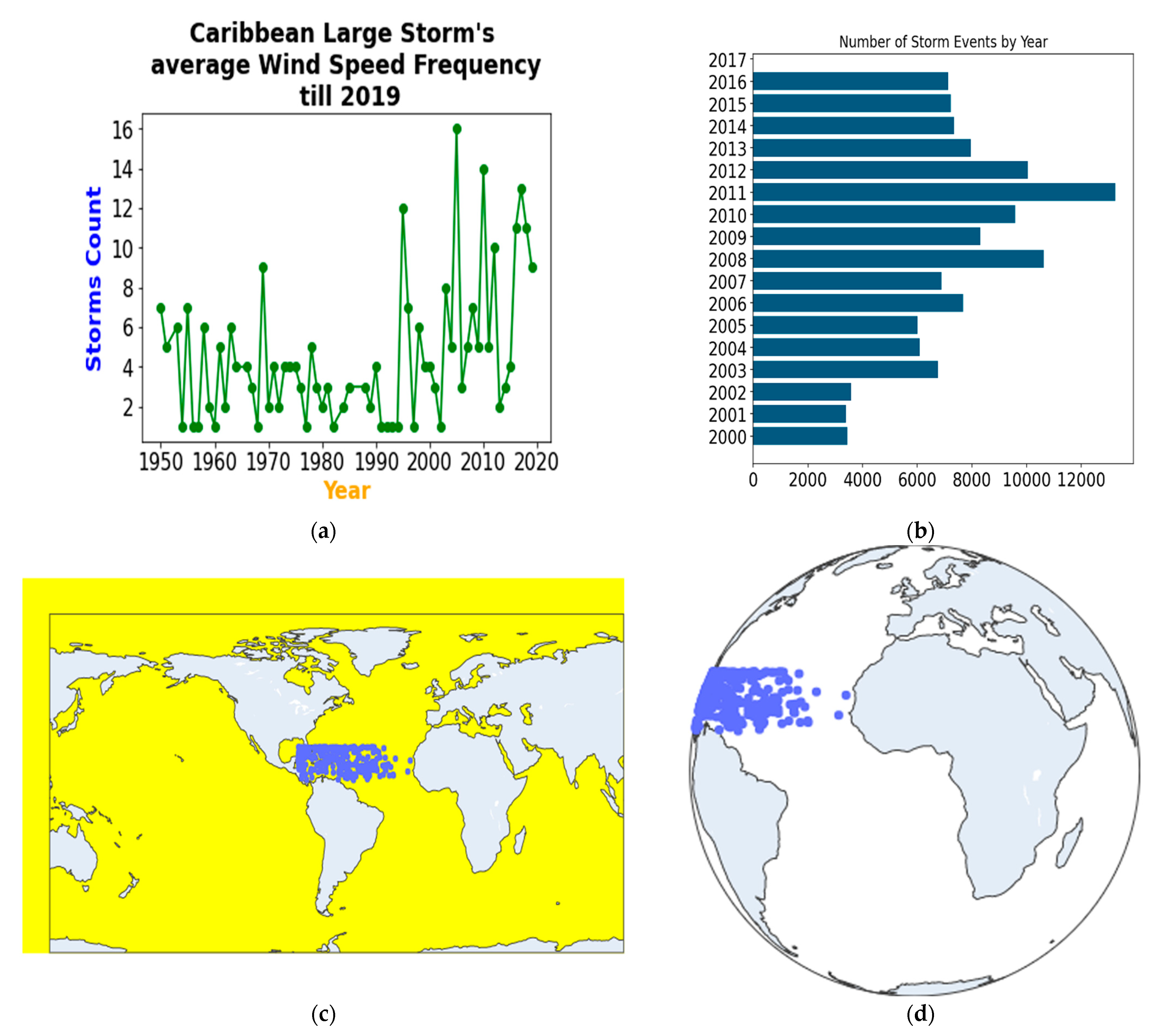
• Exploratory data analysis and visualization of hurricanes is being carried out.
• The development of improved deep CNN (I-DCNN) model for estimating the intensity using the infrared satellite imagery dataset.
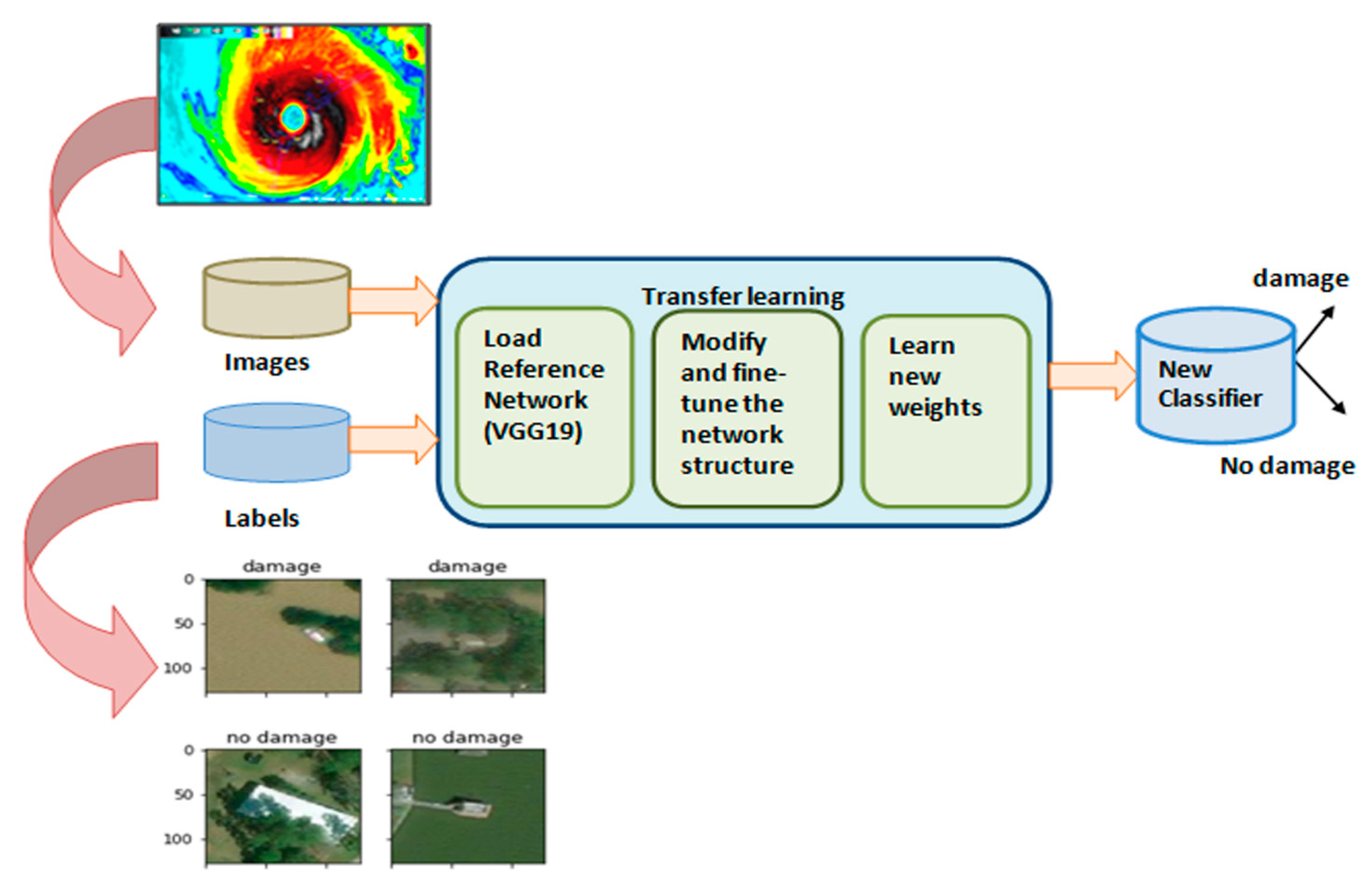
• To perform a damage assessment of hurricanes and categorization of various extreme weather events using VGG 19 CNN with data augmentation and transfer learning.
• To explore the mitigation steps in reducing the hurricane risk.

3. Methodology

This section presents the theoretical background of the related work, the dataset description and the features used to estimate the intensity and the severity of disaster, and the dataset for building damage assessment and classification of various extreme weather events with the proposed methodology.

3.1. Theoretical Background

Deep learning captures the higher-level representation of features and is widely used in computer vision, image classification, object detection, and pattern recognition algorithms. Convolutional neural networks are mostly adopted in many classification tasks [39]. Depending on the nature of the data, the features are learned by the convolutional layer. Different convolution operations are used for learning the weights of the convolution filter, which takes the input and generates the feature maps. The element-wise non-linear activation function is applied to the results. ReLU activation is used, which captures non-linearity in the network. The spatial size is reduced using the pooling layer, and it is placed between the convolution layers [40]. The average pooling or max pooling technique is used to reduce the number of parameters and to generate more abstract features using a hierarchical structure and a higher level of representation. Convolution and the pooling layers are followed by the flattened and fully connected layers with ReLU activation function. All the nodes can be fully connected to perform higher level reasoning. The back propagation algorithm stochastic gradient descent (SGD) is used to update the parameters and to learn new weights during training.

CNN has been extensively used in estimating the tropical cyclone intensity using passive microwave imagery and the hurricane database [41]. The wind speed estimates are obtained using the linear interpolation on training images. The storm track models are developed using the maximal sustained wind speed and the spatial location information. With the available computing resources, it is difficult to train the deep CNN due to the network depth and the complexity involved in classifying the data. Graphical processing units (GPUs) are mainly used for various computer vision and image classification problems by training millions of higher resolution images [42]. We extend the past work by including the infrared satellite imagery and modifying the network architecture of CNNs.

In the proposed model, max pooling layers are removed, and batch normalization layer is added after the first 2D convolution layer. With the dropout and batch normalization, the accuracy of the model is improved when compared to the existing works. The convolution operations generate the features map and apply ReLU for non-linearity, which is represented as f(x) = max(0,x).

The convolution Layer l output at position (i,j) is represented as $x_{ij}$ in Equation (1), where L X L is the size of the filter, $w_{ab}$ is the weight of the kernel at position (p,q), the receptive field is represented as $y^{l-1}{}_{\left(i+p\right)\left(j+q\right)}$ at the position (i+p),(j+q), and $B^l$ is the bias for Layer l.

$$x^l{}_{ij}={{\displaystyle \sum }}_{p=0}^{L-1}{{\displaystyle \sum }}_{q=0}^{L-1}{w}_{ab}{y}^l{}_{\left(i+p\right)\left(j+q\right)}+B^l$$

(1)

Using the hyper parameters and the size of the filters, the spatial size of the output W₀ is computed from the input W_i, the Kernel size is denoted as k with stride s and padding p which is represented in Equation (2) as

$$W_0=\frac{W_i-k+2\ast p}{s}+1$$

(2)

The normalization takes place by dividing each input $x_i$ by the total samples n and is represented in Equation (3) as follows:

$${\left(1+\frac{\propto }{n}{{\displaystyle \sum }}_i{x}_i{}^2\right)}^{\beta }$$

(3)

where α and β are the learning parameters and RMSProp optimizer is used to minimize the loss function and to learn new weights. The learning rate is adjusted automatically using the RMSProp optimizer. For each parameter, the optimizer chooses a varying learning rate. Additionally, for each parameter, the update is done and is mathematically represented in Equations (4) and (5).

$$v_t=\rho v_{t-1}+\left(1-\rho \right). g_t{}^2$$

(4)

$$\mathsf{\Delta }{w}_t=\frac{\eta }{\sqrt{v_t+\in }}\ast g_t{}^2, w_t+1=w_t+\mathsf{\Delta }{w}_t$$

(5)

where p represents the input learning parameter, ϵ is set to a small value to prevent the gradients from blowing up, η is the learning rate, and $v_t$ and $g_t$ denote the gradient squares with exponential average and the gradient, respectively, at time t.

Adam optimizer combines together the heuristics of the RMSProp and momentum. The update in the gradients of the Adam optimizer are given below in Equations (6)–(9).

$$v_t={\beta }_1\ast v_t-1-\left(1-{\beta }_1\right)\ast g_t$$

(6)

$$s_t={\beta }_2\ast s_t-1-\left(1-{\beta }_2\right)\ast g_t{}^2$$

(7)

$$\mathsf{\Delta }{w}_t=-\eta \frac{v_t}{\sqrt{s_t}+\in }\ast g_t$$

(8)

$$w_{t+1}=w_t+\mathsf{\Delta }{w}_t$$

(9)

where ${\beta }_1$ and ${\beta }_2$ are hyperparameters, $s_t$ is the exponential average of squares of gradients, and $v_t$ is the exponential average of gradients.

The comparison between the RMSProp and Adam optimizer is analyzed for hurricane intensity estimation. The dataset description and the proposed methodology are described in detail in the subsequent subsections.

3.2. Dataset Description

3.2.1. Data for Hurricane Intensity Estimation

The hurricane image database consists of the collection of satellite images (HURSAT) obtained from the National Centers for Environmental Information that are used for computing intensity prediction [43]. All the images are downloaded in NetCDF format. The hurricane is located at the center of all the images present in the database. Another dataset, called the best track data, is downloaded from the HURDAT2 database available at the National Hurricane Center [44]. Hurricanes of the Atlantic and Pacific oceans with the wind speed at 6-h interval data are present in the best track dataset. HURSAT2 data contains images of all the locations in the world, and best track data contains only wind-speed hurricane details of Atlantic and Pacific oceans. The images that match with the HURDAT2 database are only downloaded for all the years. All the satellite images are cropped and resized as a 50 × 50 square, which retains all the information without loss and also speeds up the data augmentation and model training process.

Each satellite image contains the information such as hurricane name, data, and time of satellite image, but it does not provide the hurricane wind speed details. By searching in the best track dataset by providing the name of the hurricane, the wind speed of that particular image is retrieved. Similarly, all the wind speed of the images are obtained from the HURDAT2 database. Finally, the images are labeled with the corresponding wind speed. Data augmentation is done, since the number of images of the weak tropical cyclones is greater than the number of images of strong tropical cyclones. Data augmentation is used to balance the dataset and to improve the performance. HURDAT2 best track data contains features such as location of the tropical cyclone, maximum sustained wind speed in Knots (kts), year of occurrence, and latitude and longitude at the center.

3.2.2. Data for Hurricane Damage Prediction

The data used in this study are extracted from the satellite images of the Greater Houston Area after Hurricane Harvey [45]. All the satellite images are labeled as “damaged” or “undamaged” in the building damage assessment dataset. The label “damage” indicates the images of the affected building due to the hurricane, and the label “no damage” indicates the images of the non-affected buildings. The dataset has the attributes such as the path of the image, damage status, location, and latitude and longitude. For damage prediction, a total of 5000 images are used as training data for the no damage category and 5000 images are used for the damage category. For validation and testing, 1000 files for each category were chosen for prediction. Image preprocessing is done using the packages in Keras. Good quality images are retained, and the images that are fully black or with very poor quality are automatically discarded. Simple data transformations are done using APIs to convert the string data type to float.

3.2.3. Data for Extreme Weather Event Classification

The dataset was collected from PyImageSearch with a total of 4400 Google images of different weather events such as earthquake, hurricanes, wildfires, and floods [46]. The dataset is divided into 75% for training, 25% for testing, and 10% for validation from the training split. The dataset contains a total of 928 images for cyclones, 1350 images for earthquakes, 1073 images for floods, and 1049 images for wildfires. The minimum and maximum learning rate are 1 × 10⁻⁶ and 1 × 10⁻⁴, respectively.

The prediction models used in this study are discussed in the next subsequent sections.

3.3. Methodology

This section describes the detailed proposed methodology for identifying the different categories of hurricanes based on the intensity estimation using improved deep CNN (I-DCNN), hurricane damage prediction and severe weather events using VGG19.

3.3.1. Hurricane Intensity Estimation

This section provides the details of architecture used for hurricane intensity estimation. Caribbean hurricanes are the most frequently occurring extreme weather event that impacts the Caribbean. This occurs especially due to the large volume of humidity and warm air, which are measured by the power dispersion index (PDI) and Saffir–Simpson scale. The hurricane season in the Greater Caribbean region lasts from June to November, and 85% of the hurricanes occur during the period of August and September. Upon monitoring 100 tropical depressions, it is observed that six out of 10 tropical storms turns into hurricanes every year on average. The most seasonal variability always occurs at the Atlantic Basin. The catastrophic category of damage occurred during the 2017 hurricane season in the Caribbean islands. It led to a significant loss of human life and damage to property, and the hurricane damage assessment after the disaster was carried out. The expected property damage can be predicted using the synthetic hurricane tracks [47]. Using the disturbance index, the detection of droughts and hurricane damage on the Caribbean islands is accomplished. After the hurricane Maria, a strongest hurricane hit Puerto Rico; it took 2.5 months for the recovery after the disaster [48]. The coastal regions are mostly affected by the severe storms that cause damage to human lives and property. Based on the coastal properties, the average return period is ten years for the damaging storm, and 2 percent of the storm occurrence causes destructive damages. Additionally, most of the damages are due to the storm surge and storm winds [49]. The severe hurricane rainfall events that affected the Caribbean region are due to the influence of 2 °C of global warming. The vulnerability can be assessed using three factors: susceptibility, lack of coping capacities, and lack of adaptation. These factors are used to identify the most critical areas and the crucial variables that lead to vulnerability in any specific area [50]. The total number of storms that occurred is 229 over a period of 65 years. The average wind speed over 65 years is 3.52 knots.

The most popular programming language, Python, is used for the implementation of this study. Python has a collection of pre-built libraries for image processing, scientific computing, machine learning, deep learning, data analytics, and data visualization. Complex data visualizations can be made using libraries, and visual data models can be easily created, which can help the analysts to discover the hidden patterns in the data. The libraries used for data visualization are Matplotlib, Plotly, Seaborn, GgPlot, and Geoplotlib. Matplotlib is used to embed the various kinds of plots such as scatter plots, error charts, bar charts, pie charts, histograms, etc., into the applications. Plotly provides additional plots such as contour plots, which are not present in the other data visualization libraries. Seaborn, which is based on Matplotlib, is integrated with the data structures such as Numpy and Pandas. Additionally, it provides various plots and the color palette for extracting the patterns in the data. Ggplot uses a high-level application programming interface (API) for creating the plots and isdeeply integrated with Pandas. Geoplotlib is used to create the geographical maps such as dot-density maps, symbol maps, etc., and is widely used for geographical visualizations. Keras, a deep learning framework that is built on top of TensorFlow, is used for implementation to scale a large cluster of graphical processing units (GPUs).

Figure 1a shows the bar graph of the month-wise occurrence of storms, and Figure 1b represents the plot of the year and the number of storm counts with respect to the average wind speed frequency for the Caribbean’s large storm. Figure 1c,d and Figure 2a,b depict the location of the occurrence of the hurricane and the enlarged version of the map generated using Geopandas. The attributes that denote the points in a three-dimensional space are latitude and longitude. The latitude and longitude coordinates are transformed into points, and the transition probabilities are calculated and added to the next row to determine the occurrence of the next location of the hurricane. Figure 3 shows the plot of the year and the maximum wind speed during different time periods. The heat or density maps are used to visualize the concentration of the feature in any specified area and are useful to identify the correlations between the features. Figure 4 shows the scatter plot of storms that occurred, and Figure 5 depicts the heat map with density contour until 2020. The data density can be depicted using the heatmap, and the correlation between the features are captured. For the spatial point data, the two dimensional kernel density estimation is used.

The satellite images for the Atlantic and Pacific Oceans’ hurricanes are downloaded for all the years, and the images are downloaded, to which the wind speed details are matched from the best track dataset from HURDAT2 database. The storms that do not contain the related information in the best track dataset are filtered. The satellite images from the netcdf files are extracted and stored locally. Since the hurricane is present at the center of all the images, the images are cropped at the center and matched with the maximum sustained wind speed of that hurricane. The best track dataset is filtered to search for the name, time, and date of the hurricane image. The matched images from the HURDAT2 best track data, which contains the records of Atlantic and Eastern/Central Pacific basins, are labeled with the wind speed and saved locally. The IR satellite image is retrieved from the file, the edges are removed, and the image is cropped with aside length of 50 pixels per inch (ppi).

Figure 6 shows the architecture diagram for hurricane prediction by estimating the intensity of the tropical cyclone using satellite images. The cropped images are fed to the input layers, followed by a set of convolution operations and batch normalization with dropout. Data augmentation of hurricane images is done to train the data using the convolutional neural network. K-fold validation is used to validate the model, and the augmented images for each fold are generated and combined for training. If the tropical cyclone image is within the range of 50 to 70 knots, two new images are generated. On the other hand, six new images are generated if the tropical cyclone image is within the range of 75 to 100 knots, and 12 new images are generated if the range is greater than or equal to 100 knots.

Keras Conv2D is a 2D convolution layer used to create a convolution kernel with input layers and produce the output tensors. The convolutional layers will learn from the number of filters, which is a mandatory parameter of 2D. The sequence of layers is input layers, convolution layer with activation function, pooling layers, and fully connected layers. Max pooling or average pooling is applied on the output of convolution operations to reduce the spatial dimension of the feature maps. It is used to get a small amount of translational invariance at each level. The problem associated with the pooling operation is that after applying several levels of pooling, the information about the precise positions will be lost. It is difficult to use the accurate spatial relationships between the higher-level parts of recognition. In this study, for hurricane intensity estimation, the pooling layer is replaced by a higher stride operation in the previous convolutional layer to speed up the training and reduce the computational time.

In the proposed methodology, the batch normalization layer is added after the first 2D convolution layer. The accuracy is improved by removing the max-pooling layers, and the 2D convolution layers are followed by the dropout, fully connected layers with ReLU activation, and the output layer with no activation function.

Table 3. Categories of hurricane.

Hurricane Category	Sustained Wind Speed Range (miles/h)
Tropical Depression	<=33
Tropical Storm	34–64
Category 1	74–95
Category 2	96–110
Category 3	111–130
Category 4	131–155
Category 5	>155

represents the different categories of hurricanes with respect to wind speed range in miles/h.

To reduce the loss metric value, the optimizer learns the new weights for the model. RmsProp and Adam optimizers are used to configure the model and to modify with the new weights. The mean absolute error (MAE) values are computed by plotting the training and testing loss. The different categories of hurricanes such as tropical depressions, tropical storms, and category 1, 2, 3, and 4 are plotted.

Dropout and batch normalization techniques are used to address the challenges in learning a neural network. To reduce the over-fitting of data, the regularization techniques are used, and dropouts are used to modify the network architecture randomly. For better results, dropout requires fine-tuning of the hyper-parameters. For optimizing the learning of the neural network, Adam and RMSProp are used, which are the most commonly used optimizers in Keras. Adam requires more hyper tuning, and RMSProp needs minimal tuning of parameters. Dropout increases the training convergence time, whereas the batch normalization technique helps the model to converge faster and is used to improve the efficiency of the model training. The batch normalization process improves the training time by normalizing the input at each layer. In the proposed architecture, batch normalization is added only after the first 2D convolution layer. The HURDAT2 best track data contains the input features such as storm id, storm name, year, latitude and longitude at the center, and the maximum sustained wind speed. The image with the corresponding wind speed value in the database is fed as an input to the neural network. The features are trained by the first 2D convolution layer and 32 filters with the input shape of 50 × 50. Then, batch normalization normalizes the input values followed by two 2D convolution layers with 64 filters. The output of the convolutional layers is then fed to the fully connected dense layers, and the target variable is the intensity estimation of the hurricane. Based on the intensity values, the storms are grouped into different categories, and the severity of the disaster is identified by classifying the images.

3.3.2. Dropout and Batch Normalization

If the number of training samples in the dataset is much less, it may lead to over-fitting of data, which is a significant challenge. To improve the learning rate of the model and to avoid the over-fitting of data, dropout can be added [51]. The value of dropout for the input layer is 0.1, and for the other internal layers, the dropout can be in the range of 0.5 to 0.8. Some adjustments in the hyper-parameters such as increasing the network size, learning rate, and momentum should be made after adding the dropout. If the above parameters are increased, then they will result in large weight values. To optimize the weight values, the max-norm regularization technique can be adopted.

Batch normalization improves the training speed, and the normalized values are calculated for each mini-batch. This technique increases the learning rate and is used with a lower range of values for dropout.

Figure 7 shows that the input values are normalized with the mean value as zero and standard deviation value as one. The learnable parameters ɣ and β are used with the normalized values. ɣ is the learned scaling factor, and it is initialized as 1. β is called the learned offset factor and is initialized to 0. The batch normalization technique improves the accuracy of the CNN model by incurring a very small penalty on the training time.

Figure 8 depicts the modified architecture for estimating the tropical cyclone intensity. By adding the batch normalization and dropout layers and removing the max pool layers in the CNN model, an improvement in the accuracy is obtained.

3.3.3. Hurricane Damage Prediction

This section describes the convolutional neural network used to classify the building images obtained from satellites as damaged or undamaged. The damage assessment of hurricanes is important to identify the number of flooded or damaged buildings. The image classification algorithm, such as the convolutional neural network, is employed to improve the accuracy of damage prediction. The satellite image dataset of Hurricane Harvey in 2017 is considered for hurricane damage prediction, which contains attributes such as the path of the image, damage status, location, latitude and longitude, and many others. The satellite imagery dataset is divided into training, testing, and validation, and classified as flooded/damage and undamaged. In this section, fine-tuning of the pre-trained VGG 19 is used, which gives more accuracy for the damage prediction than the existing VGG 16 model. To assess the damage caused by the occurrence of an extreme weather event, manual inspection of the satellite imagery data is tedious and time-consuming. Therefore, optical sensor imagery data with computer vision and deep learning models will be useful for analyzing the hurricane damage, which can produce accurate results. Hence, the government and other stakeholders can take necessary actions and plan for the available resources. In the satellite imagery, the affected area will be automatically annotated as “damage” or “no damage”.

Machine learning and deep learning models are the main research focus in assessing the optical sensor imagery for post-disaster assessment.

The satellite imagery data after Hurricane Harvey in the Greater Houston area are considered for training, and the images are obtained from the OpenStreetMap. Figure 9 shows the architectural diagram for hurricane building damage assessment and annotation. The reference network is loaded (VGG 19), and transfer learning takes place through which fine-tuning of the network structure is modified. The new weights are learned and updated by modifying the layers to suit our input dimension. By proper tuning of hyper parameters and optimization, the training speed can be improved [52].

For damage prediction, a total of 5000 images are used as training data for the no damage category and 5000 images are used for the damage category. For validation and testing, 1000 files for each category were chosen for prediction. Many activation functions such as Relu, tanh, sigmoid, softmax, exponential, soft sign, etc., are available, and the Relu activation function is used in the CNN and max pooling layers. In the output layer, the softmax activation function is used. The two target classes to be predicted include damage or no damage. The data is split into 70% for training and 30% for testing. Data preprocessing and data transformation are undertaken, and the labeled variables in the data are converted into a format that is understood by the model for training so that the prediction accuracy can be improved after normalizing the data. The images are cropped and resized before training, and the images are filtered to obtain the higher quality dataset. The Adam optimization algorithm is used to optimize and update the weights of the network, and training is done on the specified batch size. The errors are reduced and the performance is improved after executing every batch size. The loss function used in this study is mean square error (MSE), and epochs denote the number of iterations considered for training the dataset. The predictions are done on the test data after the training process is completed.

For hurricane damage prediction, transfer learning can be done using feature extraction, where the network is considered an arbitrary feature extractor. Another way is to fine-tune the hyper parameters, where the weights are fine-tuned to recognize the new object classes. The pre-trained model ResNet can be used as a feature extraction technique, and VGG 19 layers are used for the fine-tuning methodology. VGG 19 provides better accuracy than the ResNet pre-trained model. The images with very poor quality, fully black and very cloudy, are discarded from the dataset. Random flips and rotations on varying angles are done for the augmentation of data for training and validation. VGG 19 layers contain the consequent 2D convolution layers and 2D max pooling layers. The proposed model for hurricane damage prediction contains convolution and max pooling layers, followed by fully connected layers and the output layer. In the proposed model, VGG 19 layers are used for training, and better accuracy is achieved. Using the satellite remote sensing data, the number of flooded or damaged buildings is identified.

3.3.4. Classification of Severe Weather Events

This section describes the automatic detection and classification of weather events such as hurricanes, earthquakes, floods, and wildfires. A deep convolutional neural network called visual geometry group VGG 19, a successor of AlexNet, is used to classify the weather events [53]. The data are trained from the ImageNet, and the class labels in the datasets are initialized. Additionally, classification using video streams of weather events are tested and demonstrated. The minimum and maximum learning rate are specified as 1 × 10⁻⁶ and 1 × 10⁻⁴, respectively. The batch size and the step size are chosen as 32 and 8. The triangular cyclic learning rate method is adopted, which provides the best learning rate using the LR (learning rate) range test. The LR range test includes the step size, maximum bound value, and the minimum bound value. After each cycle, the learning rate difference is dropped in the triangular learning rate policy. Keras learning rate finder is used to find the optimal learning rates for fine-tuning the VGG 19 CNN on the dataset. Starting at the lower bound, the training of the network takes place, and the learning rate is increased exponentially after each batch update. The training is continued until the maximum learning rate is achieved. Once the initial batch is completed, the learning rate for the next batch is increased.

3.4. VGG 19 Architecture

Images in the dataset are converted to a fixed size of (224 × 224) RGB image and are given as inputs to the VGG 19 network. The preprocessing is done by subtracting the mean RGB value from each pixel, which is calculated from the whole training data. Kernels of 3 × 3 size with a stride size of one pixel are used, and to retain the spatial resolution of the image, spatial padding is used. Additionally, Max pooling was performed over 2 × 2 pixel windows with a stride of 2. In order to introduce the non-linearity and to improve the computational time, the rectified linear unit (ReLU) is followed by the max pooling layers. Three fully connected layers with the ReLU activation function are used, and the final layer is the output layer with the Softmax function.

Figure 10 shows the layered architecture of VGG 19. The optimal learning rate is used with the cyclic learning rates to obtain high accuracy, and faster convergence takes place with CLR. The resized images are added to the data list after preprocessing. One hot encoding is done to convert the labels to an array, and the data are converted to float values. VGG 19 is loaded using the pre-trained ImageNet weights followed by the creation of fully connected layers added to VGG 19. The data augmentation object is instantiated, and the training is done on the whole dataset. Good accuracy is obtained by fine-tuning the layers from 15 to 19.

The proposed models are assessed using various performance metrics, which is elaborated in the next section.

4. Performance Metrics and Evaluation

All the models proposed in this study are implemented using Tensorflow, Keras, and Scikit-learn. The number of epochs run for the model is 100, with a batch size of 64. The models were trained and tested on the dependent features of satellite images and the HURDAT2 data. The data are split into 70% for training, 20% for testing, and 10% for validation. To evaluate the performance of the models, the metrics used are mean absolute error (MAE), mean absolute percentage error (MAPE), mean squared error (MSE), and root mean squared error (RMSE). In the below specified equations, the predicted output and the actual values are represented.

$$MAE=\frac{1}{N}{{\displaystyle \sum }}_{i=1}^N\left(\overline{x_i}-x_i\right)$$

(10)

$$Relative RMSE=\frac{\sqrt{{\left(x_p-x_t\right)}^2}}{\frac{n-1}{\overline{X_p}}}$$

(11)

$$MSE=\frac{1}{N} {{\displaystyle \sum }}_{i=1}^N{\left(\overline{x_i}-x_i\right)}^2$$

(12)

$$RMSE=\sqrt{\frac{1}{N}}{{\displaystyle \sum }}_{i=1}^N{\left(\overline{x_i}-x_i\right)}^2.$$

(13)

The proposed models are evaluated based on the above metrics given in Equations (10)–(13). The performance metric used for classification is the confusion matrix, which describes about four categories of data, i.e., true positives (TP), true negatives (TN), false positives (FP), and false negatives (FN). The success–failure ratio is determined by the confusion matrix.

When the speed of the wind increases and exceeds a certain threshold value, then severe weather events cause serious damages to human lives, property, and crops. The performance metrics computed for the damage prediction are precision, recall, F1 score, false alarm rate (FAR), probability of detection (POD), and critical success index (CSI), as given in Equations (14)–(18).

Precision: It is the ratio of actual positive identifications to the total actual hailstorm or hurricane and no hailstorm or no hurricane.

$$Precision=\frac{TP}{TP+FP}$$

(14)

Recall: It is the ratio of the actual positive identifications to the summation of total positive and false positive values.

$$Recall=\frac{TP}{TP+FN}$$

(15)

F1 score: It is the measure of the test’s accuracy and is calculated from the precision and recall.

$$F1 Score=2·\frac{precision·recall}{precision+recall}=\frac{TP}{TP+1/2\left(FP+FN\right)}$$

(16)

For the critical success index (CSI), also called the threat score (TS), a measure of categorical forecast performance is computed as

$$CSI=\frac{FP}{TP+FP}$$

(17)

The false alarm rate (FAR) is also called the probability of false detection and is computed as

$$FAR=\frac{TP}{TP+TN+FP+FN}$$

(18)

The prediction results of all the models are presented in the subsequent section.

5. Results and Discussions

5.1. Prediction of Hurricane Intensity

This section depicts the results of predicting the hurricane intensity using the improved CNN model.

The accuracy of the modified CNN architecture for estimating the hurricane intensity using Infrared satellite imagery for Atlantic and Pacific regions is depicted in Figure 11a–e. Recent studies use various types of CNN models such as VGG, AlexNet, ResNet, and InceptionNet depending on the dataset and the number of convolutional layers used for predicting the intensity and classifying the damages caused after disaster. Root mean square error (RMSE) and mean squared error loss (MSE) values are computed, and the error values of the k-fold validation is represented in

Table 4. RMSE values for k-fold validation.

Validation Fold	Fold 1	Fold 2	Fold 3	Fold 4	Fold 5
RMSE	17.8 knots	17.4 knots	8.2 knots	8.1 knots	7.6 knots

, where the value of k is 5. Table 4 describes about five-fold validation, and the lower RMSE values are arrived at with 7.6 knots. The batch normalization normalizes each input after the first 2D convolution layer by computing the mean and variance value. Error values are higher before removing max pooling layers. After removing the max pooling layers and increasing the stride value of the previous convolutional layer, the error values are reduced.

Figure 12 depicts the absolute error values of the different categories of hurricanes based on the intensity estimation of the satellite images. The hurricane strength and the absolute error values are plotted. Totally, 248 samples are tested for tropical depressions, 355 samples for tropical storms, 55 samples for category 1, 19 samples for category 2, 13 samples for category 3, and three samples for category 4. By training the proposed model, the lower error values are achieved through better model initialization of the input by estimating the intensity values. The sample images at different knots using data augmentation and transfer learning are depicted in Figure 13a,b. Two new images are generated if the tropical cyclone intensity value is less than 75 knots. Six new images are generated if the intensity value is between 75 and 100 knots.

Table 5. Performance evaluation using different optimizers.

Optimizer/Technique Used	Mean Absolute Error (MAE) Knots	Root Mean Square Error (RMSE) Knots	Relative RMSE
RMSProp (no max-pooling, no batch normalization, and only dropout)	7.21 kts	9.47 kts	0.19
RMSProp (no max-pooling, with batch normalization and dropout)	6.68 kts	7.6 kts	0.17
Adam optimizer (no max-pooling, no batch normalization, and only dropout)	8.68 kts	10.18 kts	0.22
Adam optimizer (no max-pooling, with batch normalization and dropout)	8.52 kts	10.04 kts	0.20

shows the performance evaluation using the optimizers Adam and RMSProp. Optimizers are used to learn the new weights and the learning rates in the network and to minimize the loss. RMSProp is the gradient-based optimization technique, which is used to balance the step size through the normalization process and avoids the vanishing gradient problem. Adam optimizers are used to handle the sparse gradients and are slower to change their direction. Twelve new images are generated if the value is greater than 100 knots. The results of the Adam optimizer are slightly higher than the RMSProp, and the RMSProp optimizer provides good results with lower RMSE values. Overall, removing max pooling layers provides better results. The addition of batch normalization and dropout layers further improves the performance. The optimizer performances with different techniques are compared in Table 5. The best performance result is obtained for the combined techniques of removing the max pooling layers and adding the batch normalization with dropout. A MAE value of 6.68 knots and an RMSE value of 7.6 knots are obtained using the proposed technique.

5.2. Hurricane Damage Prediction

This section presents the results and analysis of hurricane damage prediction after Hurricane Harvey in 2017. The satellite imagery data are divided into training, testing, and validation.

In Figure 14, training, testing, and validation split, and the labels with the damage and no damage classes with respect to latitude and longitude are plotted. The validation split is considered from the training split data. Figure 15 shows the distribution of RGB values. In the histogram, the x-axis is split into number ranges or the bins where the width of the bar represents the range of the bin and the height represents the total number of data points that lies within that range. The y-axis represents the frequency or count of the distribution of components in a particular bin. Figure 16 shows the sample images of damage/no damage classes. Data transformation takes place where the data are converted to float32 and scaling is done from an unsigned integer in the range of 0 to 255 to float32 with normalized values between 0 to 1. Image augmentation is applied by rotating through 90, 180, or 270 degrees with random flips. The augmented and the original datasets are merged together. The number of samples in the training and validation sets are doubled using image augmentation. Figure 17 shows the results after data preprocessing, where the original dataset is transformed to the RGB format. Initially, the batch size is fixed as 32, and the base model is created from the pre-trained model VGG 19. It converts 128 × 128 × 3 image to a 4 × 4 × 512 set of feature blocks.

Table 6. Configuration of VGG 19 layers.

Layer (Type)	Output Shape	Param #
input_1 (InputLayer)	[(None, 128, 128, 3)]	0
block1_conv1 (Conv2D)	(None, 128, 128, 64)	1792
block1_conv2 (Conv2D)	(None, 128, 128, 64)	36,928
block1_pool (MaxPooling2D)	(None, 64, 64, 64)	0
block2_conv1 (Conv2D)	(None, 64, 64, 128)	73,856
block2_conv2 (Conv2D)	(None, 64, 64, 128)	147,584
block2_pool (MaxPooling2D)	(None, 32, 32, 128)	0
block3_conv1 (Conv2D)	(None, 32, 32, 256)	295,168
block3_conv2 (Conv2D)	(None, 32, 32, 256)	590,080
block3_conv3 (Conv2D)	(None, 32, 32, 256)	590,080
block3_conv4 (Conv2D)	(None, 32, 32, 256)	590,080
block3_pool (MaxPooling2D)	(None, 16, 16, 256)	0
block4_conv1 (Conv2D)	(None, 16, 16, 512)	1,180,160
block4_conv2 (Conv2D)	(None, 16, 16, 512)	2,359,808
block4_conv3 (Conv2D)	(None, 16, 16, 512)	2,359,808
block4_conv4 (Conv2D)	(None, 16, 16, 512)	2,359,808
block4_pool (MaxPooling2D)	(None, 8, 8, 512)	0
block5_conv1 (Conv2D)	(None, 8, 8, 512)	2,359,808
block5_conv2 (Conv2D)	(None, 8, 8, 512)	2,359,808
block5_conv3 (Conv2D)	(None, 8, 8, 512)	2,359,808
block5_conv4 (Conv2D)	(None, 8, 8, 512)	2,359,808
block5_pool (MaxPooling2D)	(None, 4, 4, 512)	0
Total params: 20,024,384 Trainable params: 0 Non-trainable params: 20,024,384

and

Table 7. Trainable and non-trainable parameters. Model: “sequential”.

Model: “Sequential” Layer (type)	Output Shape	Param #
Vgg19 (Model) Global_averge_pooling2d dense (Dense)	(None, 4, 4, 512) G1(None, 512) (None, 1)	20,024,384 0 513
Total params: 20,024,384 Trainable params: 513 Non-trainable params: 20,024,384

represent the configuration of VGG 19 layers, and the total number of trainable and non-trainable parameters are found after average pooling and dense layers.

Table 8. Configuration details and number of parameters. Model: “sequential”.

Model: “Sequential” Layer (Type)	Output Shape	Param #
Vgg19 (Model) Global_averge_pooling2d dense (Dense)	(None, 4, 4, 512) G1(None, 512) (None, 1)	20,024,384 0 513
Total params: 20,024,384 Trainable params: 7,079,937 Non-trainable params: 12,944,960

shows the number of trainable and non-trainable parameters after fine-tuning the VGG 19 layers. Transfer learning can be achieved through feature extraction or fine-tuning of layers. Fine-tuning of the layers outperforms the feature extractor technique and provides higher accuracy. Initially, by training the network with the small learning rate, and through the previously learned convolutional layers, a new set of fully connected layers can learn the patterns. Applying fine-tuning leads to higher accuracy, the last few layers of VGG 19 from the layer 15 to layer 19 are fine-tuned for damage prediction, and automatic annotation of the images is done using the model. The baseline model achieves about 80% accuracy before fine-tuning the layers and is represented in Figure 18. After fine-tuning, the model with 98% accuracy is achieved using VGG 19 and is represented in Figure 19. The critical success index (CSI) is 0.80 and the false alarm rate (FAR) for hurricane damage detection is 0.91.

Table 9. Comparative analysis of existing models.

Ref	Disaster Type	Dataset	Model Used	Accuracy
[54]	Hurricane	Hurricane satellite images	Deep CNN	80.66%
[55]	Flood	Flood video dataset	Base CNN	70%
[56]	Hurricane	AIDR dataset	VGG-16	74%
[57]	Hurricane	Hurricane Sandy dataset	Convolutional Auto-encoders	88.4%
[58]	Hurricane	Hurricane Harvey	VGG 16 CNN	89.5%
Proposed	Hurricane	Hurricane Harvey	VGG 19 CNN (with fine-tuning)	98%

shows the comparative analysis of existing models and the proposed model. Fine-tuning VGG 19 layers gives the improved accuracy, and it outperforms the other existing techniques.

5.3. Detection and Annotation of Severe Weather Events

This section discusses the detection and annotation of different types of severe weather events using the pre-trained network. The dataset was collected from the PyimageSearch with a total of 4400 Google images of different weather events. The dataset is divided into 75% for training, 25% for testing, and 10% for validation from the training split. Classification using video streams of weather events is tested and demonstrated.

Figure 20 shows the learning rate with the maximum and minimum bounds. The optimal learning rate is found between 1 × 10⁻⁶ to 1 × 10⁻⁴, since the loss value drops until 1 × 10⁻⁴ and starts increasing after that, which leads to over-fitting. After fine-tuning the last few layers, the accuracy of the model is increased, and 97% accuracy is achieved in detecting the severe weather events. Figure 21a shows that the validation loss follows the training loss, implying that there is very little over-fitting in the original dataset itself. Figure 21b shows the accuracy graph. Figure 22 shows the learning plot where the cyclical learning rate (CLR) callback is depicted between the optimal range of LR test. The trained model is tested over images and videos of weather events, which have similar semantic contents. The predictions queue, video streams, and the frame dimensions are initialized. The frames of the video streams are stored and resized to the fixed size of 224 × 224. The automatic annotation of the frame is done by extracting the highest probability class label for the predictions in the queue.

Table 10. Layers of VGG19.

Layer (Type)	Output Shape	Param #
input_1 (Input Layer)	(None, 224, 224, 3)	0
block1_conv1 (Conv2D)	(None, 224, 224, 64)	1792
block1_conv2 (Conv2D)	(None, 224, 224, 64)	36,928
block1_pool (MaxPooling2D)	(None, 112, 112, 64)	0
block2_conv1 (Conv2D)	(None, 112, 112, 128)	73,856
block2_conv2 (Conv2D)	(None, 112, 112, 128)	147,584
block2_pool (MaxPooling2D)	(None, 56, 56, 128)	0
block3_conv1 (Conv2D)	(None, 56, 56, 256)	295,168
block3_conv2 (Conv2D)	(None, 56, 56, 256)	590,080
block3_conv3 (Conv2D)	(None, 56, 56, 256)	590,080
block3_conv4 (Conv2D)	(None, 56, 56, 256)	590,080
block3_pool (MaxPooling2D)	(None, 28, 28, 256)	0
block4_conv1 (Conv2D)	(None, 28, 28, 512)	1,180,160
block4_conv2 (Conv2D)	(None, 28, 28, 512)	2,359,808
block4_conv3 (Conv2D)	(None, 28, 28, 512)	2,359,808
block4_conv4 (Conv2D)	(None, 28, 28, 512)	2,359,808
block4_pool (MaxPooling2D)	(None, 14, 14, 512)	0
block5_conv1 (Conv2D)	(None, 14, 14, 512)	2,359,808
block5_conv2 (Conv2D)	(None, 14, 14, 512)	2,359,808
block5_conv3 (Conv2D)	(None, 14, 14, 512)	2,359,808
block5_conv4 (Conv2D)	(None, 14, 14, 512)	2,359,808
block5_pool (MaxPooling2D)	(None, 7, 7, 512)	0
flatten (Flatten)	(None, 25,088)	0
dense (Dense)	(None, 512)	12,845,568
dropout (Dropout)	(None, 512)	0
dense_1 (Dense)	(None, 4)	2052
Total params: 32,872,004
Trainable params: 12,847,620
Non-trainable params: 20,024,384

shows the layer type, output shape, and the number of parameters in VGG 19 layers. The input image is processed by the convolutional layers, followed by nonlinear transforming unit ReLU and a pooling layer. The low-level features can be extracted in the deep learning models through down sampling, which can be achieved by the pooling layers. ReLU is applied to the feature maps generated by the convolutional layers. The pooling layer operates on each feature map and generates a new set of pooled feature maps. The pooling layer will reduce the size of the feature map by a factor of 2, and max pooling computes the maximum value in the set of feature maps. The total number of parameters, the number of trainable and non-trainable parameters using VGG 19, is shown in the table.

Table 11. Performance evaluation for the classification of severe weather events using VGG 19.

	Precision	Recall	F1-Score	Support
Hurricane	0.98	0.96	0.97	207
Earthquake	0.96	0.93	0.95	364
Flood	0.91	0.94	0.93	265
Wildfire	0.97	0.98	0.97	249
Accuracy			0.96	1107

shows the performance evaluation of various metrics for classifying different types of weather events.

Figure 23 shows the detection of severe weather events with the annotation of video clips in real-time. The rolling frame classification technique is used, where the rolling average forecast is computed using the standard average. The first calculated average is the simple standard average, and the forecast after the first standard average forecast is called the rolling average prediction. It denotes the process of moving the average value to the next set of n periods of frames. In the datasets collected, there is temporal and semantic similarity between the frames of the video streams and so the average rolling classification approach provides good results. Since the video datasets of different events have temporal correlations and semantic similarities, the high accuracy of 97% is obtained. Figure 23 shows the live detection and annotation of severe weather events using the VGG 19 CNN model. Ninety-seven percent accuracy is achieved after fine-tuning the last five layers.

5.4. Hurricane Risk Mitigation

It is important to understand the risk imposed due to the occurrence of hurricanes and to take necessary steps to avoid significant losses. Human lives can be saved and economic losses can be reduced by implementing the policies and measures in advance and by imparting awareness to the public. The hurricane risk in the Caribbean and Central America is high. Due to the technological advancement in prediction models, the tropical depression can be predicted accurately, and an early warning can be given to the public. Countries can include the mitigation measures by considering the details such as distribution of the occurrence of hurricanes, wind speed and direction, height of the storm surges, etc. The mitigation measures adopted should consider the long-term effects. Additionally, hurricanes cause serious health hazards to people and lead to various types of diseases. The disease incurred might last for months or even years. Building codes can be used to control the building designs, methods, and materials. Formulating the mitigation strategy is an essential step in vulnerability analysis and risk assessment.

6. Conclusions and Future Work

In this work, the deep learning models are developed to estimate the tropical cyclone intensity and to identify the severity of different categories of hurricane. The conclusions of this exertion are summarized as follows:

• For hurricane intensity estimation, an improved deep CNN model is trained with the satellite images of hurricane along with the wind speed data. The proposed model provides lower RMSE value of 7.6% and MAE value of 6.68% after removing the max-pooling layers, and adding the batch normalization after first convolution layer.
• For building damage assessment in context with post-disaster management, transfer learning using feature extraction of VGG 19 CNN achieves a higher accuracy of 98% than VGG 16 model, with most of the predictions as true positives.
• For classifying the severe weather events, fine-tuning of VGG 19 achieves a higher accuracy of 97% by training the video datasets
• Importance of mitigation measures against hurricane are addressed.

The National Ocean and Atmospheric Administration (NOAA) and the National Hurricane Center (NHC) use different tools to predict the intensity of storms. For predicting the trajectory and strength of the hurricane, it is necessary to understand the structure of the storm and its location. Deep learning models help to accurately forecast the storm intensity at various levels, which helps the government to prevent hazards. To predict the hurricane damage prediction and the loss incurred is difficult, because it mainly depends on the storm severity and the vulnerability of the area the hurricane hits. Hurricanes also threaten the water and sewer systems, flood management, and transportation, in addition to the damages caused by the buildings. Strong hurricanes cause a high risk to public health and human lives, since within a shorter span of time, intensity changes may occur that may lead to human death and damages to property. The prediction of intensity levels using deep learning models provides an earlier warning of the storm formation. The potential future work includes adding a greater number of layers and improving the performance of the proposed model. The hurricane is located at the center of all the images, and there are various challenges related to data preprocessing, such as the removal of noise and distortion removal. It can be improved using efficient pre-processing techniques to enhance the efficiency of the prediction model. Additionally, severe weather events’ impact across different countries should be controlled by designing the mitigation steps and including them in the development plan.

References

1. Smith, G. Hurricane names: A bunch of hot air? Weather Clim. Extrem. 2016, 12, 80–84. [Google Scholar] [CrossRef] [Green Version]
2. Schwartz, S.B. Sea of Storms: A History of Hurricanes in the Greater Caribbean from Columbus to Katrina; Princeton University Press: Princeton, NJ, USA, 2015. [Google Scholar]
3. Mori, N.; Takemi, T. Impact assessment of coastal hazards due to future changes of tropical cyclones in the North Pacific Ocean. Weather Clim. Extrem. 2016, 11, 53–69. [Google Scholar] [CrossRef] [Green Version]
4. Karpatne, A.; Ebert-Uphoff, I.; Ravela, S.; Babaie, H.; Kumar, V. Machine learning for the geosciences: Challenges and opportunities. IEEE Trans. Knowl. Data Eng. 2019, 31, 1544–1554. [Google Scholar] [CrossRef] [Green Version]
5. Zipser, E.; Liu, C.; Cecil, D.; Nesbitt, S.; Yorty, S. Where are the most intense thunderstorms on Earth? Bull. Am. Meteorol. Soc. 2006, 87, 1057–1071. [Google Scholar] [CrossRef] [Green Version]
6. Gagne, D.J., II; Williams, J.K.; Brown, R.A.; Basara, J.B. Enhancing understanding and improving prediction of severe weather through spatiotemporal relational learning. Mach. Learn. 2014, 95, 27–50. [Google Scholar] [CrossRef] [Green Version]
7. McGovern, A.; Elmore, K.L.; Gagn, D.J., II; Haupt, S.E.; Karstens, C.D.; Lagerquist, R.; Smith, T.; Williams, J.K. Using Artificial Intelligence to improve real-time decision making. Bull. Am. Meteorol. Soc. 2017, 98, 2073–2090. [Google Scholar] [CrossRef]
8. Olander, T.; Velden, C. The current status of the UW-CIMSS Advanced Dvorak Technique (ADT). In Proceedings of the 30th Conference Hurricanes Tropical Meteorology, Madison, WI, USA, 17 April 2012; American Meteorological Society: Boston, MA, USA, 2012. [Google Scholar]
9. Olander, T.; Velden, C. The advanced Dvorak technique: Continued development of an objective scheme to estimate tropical cyclone intensity using geostationary infrared satellite imagery. Weather Forecast. 2007, 22, 287–298. [Google Scholar] [CrossRef]
10. Olander, T.; Velden, C. The advanced Dvorak technique (ADT) for estimating tropical cyclone intensity: Update and new capabilities. Weather Forecast. 2019, 34, 905–922. [Google Scholar] [CrossRef]
11. Pineros, M.; Ritchie, E.; Tyo, J. Estimating tropical cyclone intensity from infrared image data. Weather Forecast. 2011, 26, 690–698. [Google Scholar] [CrossRef]
12. Pineros, M.; Ritchie, E.; Tyo, J. Objective measures of tropical cyclone structure and intensity change from remotely sensed infrared image data. IEEE Trans. Geosci. Remote Sens. 2008, 46, 3574–3580. [Google Scholar] [CrossRef]
13. Ritchie, E.; Valliere-Kelley, G.; Piñeros, M.; Tyo, J. Tropical cyclone intensity estimation in the North Atlantic basin using an improved deviation angle variance technique. Weather Forecast. 2012, 27, 1264–1277. [Google Scholar] [CrossRef] [Green Version]
14. Ritchie, E.; Wood, K.; Rodríguez-Herrera, O.; Pineros, M.; Tyo, J. Satellite-derived tropical cyclone intensity in the North Pacific Ocean using the deviation-angle variance technique. Weather Forecast. 2014, 29, 505–516. [Google Scholar] [CrossRef] [Green Version]
15. Li, L.; Zhou, Y.; Wang, H.; Zhou, H.; He, X.; Wu, T. An Analytical Framework for the Investigation of Tropical Cyclone Wind Characteristics over Different Measurement Conditions. Appl. Sci. 2019, 9, 5385. [Google Scholar] [CrossRef] [Green Version]
16. Hay, J.; Mimura, N. The changing nature of extreme weather and climate events: Risks to sustainable development. Geomat. Nat. Hazards Risk 2010, 1, 3–18. [Google Scholar] [CrossRef]
17. Devaraj, J.; Elavarasan, R.M.; Pugazhend, R.; Shafiullah, G.M.; Ganesan, S.; Jeysree, A.K.; Khan, I.A.; Hossain, E. Forecasting of COVID-19 cases using deep learning models: Is it reliable and practically significant? Results Phys. 2021, 21, 103817. [Google Scholar] [CrossRef] [PubMed]
18. Raz, T.; Liwag, C.R.E.U.; Valentine, A.; Andres, L.; Castro, L.T.; Cuña, A.C.; Vinarao, C.; Raza, T.K.S.; Mchael, K.; Marsian, E.; et al. Extreme weather disasters challenges for sustainable development: Innovating a science and policy framework for disaster-resilient and sustainable, Quezon City, Philippines. Prog. Disaster Sci. 2020, 5, 100066. [Google Scholar] [CrossRef]
19. Bao, X.; Jiang, D.; Yang, X.; Wang, H. An improved deep belief network for traffic prediction considering weather factors. Alex. Eng. J. 2021, 60, 413–420. [Google Scholar] [CrossRef]
20. Devaraj, J.; Elavarasan, R.M.; Shafiullah, G.M.; Jamal, T.; Khan, I. A holistic review on energy forecasting using big data and deep learning models. Int. J. Energy Res. 2021. [Google Scholar] [CrossRef]
21. Anbarasana, M.; Muthu, B.A.; Sivaparthipan, C.B.; Sundarasekar, R.; Dine, S. Detection of flood disaster system based on IoT, big data and convolutional deep neural network. Comput. Commun. 2020, 150, 150–157. [Google Scholar] [CrossRef]
22. Rysman, J.L.L.; Claud, C.; Dafis, S. Global monitoring of deep convection using passive microwave observations. Atmos. Res. 2021, 247, 105244. [Google Scholar] [CrossRef]
23. Tien, D.; Nhat-DucHoang, D.; Martínez-Álvarez, F.; Thi Ngo, P.; Viet Hoa, P.; Dat Pham, T.; Samui, P.; Costacheij, R. A novel deep learning neural network approach for predicting flash flood susceptibility: A case study at a high frequency tropical storm area. Sci. Total Environ. 2020, 701, 134413. [Google Scholar] [CrossRef]
24. Kordmahalleh, M.M.; Sefidmazgi, M.G.; Homaifar, A.A. A Sparse Recurrent Neural Network for Trajectory Prediction of Atlantic Hurricanes. In Proceedings of the Genetic and Evolutionary Computation Conference (GECCO’ 16), Denver, CO, USA, 20–24 July 2016; pp. 957–964. [Google Scholar]
25. Mangalathu, S.; Burton, H.V. Deep learning-based classification of earthquake-impacted buildings using textual damage descriptions. Int. J. Disaster Risk Reduct. 2019, 36, 101111. [Google Scholar] [CrossRef]
26. Alemany, S.; Beltran, J.; Perez, A.; Ganzfried, S. Predicting Hurricane Trajectories Using a Recurrent Neural Network. In Proceedings of the Thirty-Third AAAI Conference on Artificial Intelligence (AAAI-19), Honolulu, HI, USA, 27 January–1 February 2019. [Google Scholar]
27. Chen, R.; Wang, X.; Zhang, W.; Zhu, X.; Li, A.; Yang, C. A hybrid CNN-LSTM model for typhoon formation forecasting. Geoinformatica 2019, 23, 375–396. [Google Scholar] [CrossRef]
28. Mohammadi, M.E.; Watson, D.P.; Wood, R.L. Deep Learning-Based Damage Detection from Aerial SfM Point Clouds. Drones 2019, 3, 68. [Google Scholar] [CrossRef] [Green Version]
29. Zhou, K.H.; Zheng, Y.G.; Li, B. Forecasting different types of convective weather: A deep learning approach. J. Meteorol. Res. 2019, 33, 797–809. [Google Scholar] [CrossRef]
30. Snaiki, R.; Wu, T. Knowledge-enhanced deep learning for simulation of tropical cyclone boundary-layer winds. J. Wind Eng. Ind. Aerodyn. 2019, 194, 103983. [Google Scholar] [CrossRef]
31. Chen, B.F.; Chen, B.; Elsberry, R.L. Estimating Tropical Cyclone Intensity by Satellite Imagery Utilizing Convolutional Neural Networks. Weather Forecast. 2019, 34, 447–465. [Google Scholar] [CrossRef]
32. Castro, R.; Souto, Y.M.; Ogasawara, E.; Porto, F.; Bezerra, E. STConvS2S: Spatiotemporal Convolutional Sequence to Sequence Network for weather forecasting. Neurocomputing 2020, 426, 285–298. [Google Scholar] [CrossRef]
33. Kim, S.; Kim, H.; Lee, J.; Yoon, S.W.; Kahou, S.E.; Kashinath, K.; Prabhat, M. Deep-Hurricane-Tracker: Tracking and Forecasting Extreme Climate Events. In Proceedings of the IEEE Winter Conference on Applications of Computer Vision (WACV), Waikoloa Village, HI, USA, 7–11 January 2019. [Google Scholar]
34. Li, Y.; Hu, W.; Dong, H.; Zhang, X. Building Damage Detection from Post-Event Aerial Imagery Using Single Shot Multibox Detector. Appl. Sci. 2019, 9, 1128. [Google Scholar] [CrossRef] [Green Version]
35. Haghroosta, T. Comparative study on typhoon’s wind speed prediction by a neural networks model and a hydrodynamical model. MethodsX 2019, 6, 633–640. [Google Scholar] [CrossRef]
36. Chen, Y.; Zhang, S.; Zhang, W.; Peng, J.; Cai, Y. Multifactor spatio-temporal correlation model based on a combination of convolutional neural network and long short-term memory neural network for wind speed forecasting. Energy Convers. Manag. 2019, 185, 783–799. [Google Scholar] [CrossRef]
37. Neshat, M.; Nezhad, M.M.; Abbasnejad, E.; Mirjalili, S.; Tjernberg, B.L.; Garcia, A.D.; Alexander, B.; Wagner, M. A deep learning-based evolutionary model for short-term wind speed forecasting: A case study of the Lillgrund offshore wind farm. Energy Convers. Manag. 2021, 236, 114002. [Google Scholar] [CrossRef]
38. Meka, R.; Alaeddini, A.; Bhaganagar, K. A robust deep learning framework for short-term wind power forecast of a full-scale wind farm using atmospheric variables. Energy 2021, 221, 119759. [Google Scholar] [CrossRef]
39. Krizhevsky, A.; Sutskever, I.; Hinton, G. ImageNet classification with deep convolutional neural networks. In Proceedings of the NIPS’12 Information Processing Systems, Lake Tahoe, NV, USA, 3–6 December 2012; Volume 1, pp. 1097–1105. [Google Scholar]
40. Bengio, Y.; Courville, A. Deep learning of representations. In Handbook on Neural Information Processing; Springer: Berlin, Germany, 2013; Volume 49, pp. 1–28. [Google Scholar]
41. Pradhan, R.; Aygun, R.; Maskey, M.; Ramachandran, R.; Cecil, D. Tropical cyclone intensity estimation using a deep convolutional neural network. IEEE Trans. Image Process. 2018, 27, 692–702. [Google Scholar] [CrossRef] [PubMed]
42. Zeiler, M.D.; Fergus, R. Visualizing and Understanding Convolutional Networks. In Computer Vision—ECCV 2014; Fleet, D., Pajdla, T., Schiele, B., Tuytelaars, T., Eds.; Springer: Zurich, Switzerland, 2014; pp. 818–833. [Google Scholar]
43. Dataset for Hurricane Is Accessed from NHC. Available online: https://www.nhc.noaa.gov/ (accessed on 20 November 2020).
44. Satellite Imagery Data Are Accessed from HURSAT2. Available online: https://www.ncdc.noaa.gov/hursat/ (accessed on 20 November 2020).
45. Satellite Dataset for Hurricane Damage Prediction Is Accessed from IEEE DataPort. Available online: https://ieee-dataport.org/keywords/hurricane (accessed on 20 November 2020).
46. Classification of Extreme Weather Events Dataset from pySearchImage GoogleImages. Available online: https://www.pyimagesearch.com (accessed on 30 December 2020).
47. Bertinelli, L.; Mohan, P.; Strobl, E. Hurricane damage risk assessment in the Caribbean: An analysis using synthetic hurricane events and nightlight imagery. Ecol. Econ. 2016, 124, 135–144. [Google Scholar] [CrossRef]
48. Beurs, K.M.; McThompson, N.S.; Owsley, B.C.; Henebry, G.M. Hurricane damage detection on four major Caribbean islands. Remote Sens. Environ. 2019, 229, 1–13. [Google Scholar] [CrossRef]
49. Sealya, K.; Strobl, E. A hurricane loss risk assessment of coastal properties in the caribbean: Evidence from the Bahamas. Ocean Coast. Manag. 2017, 149, 42–51. [Google Scholar] [CrossRef]
50. Medina, N.; Abebe, Y.A.; Sanchez, A.; Vojinovic, Z. Assessing Socio economic Vulnerability after a Hurricane: A Combined Use of an Index-Based approach and Principal Components Analysis. Sustainability 2020, 12, 1452. [Google Scholar] [CrossRef] [Green Version]
51. Srivastava, N.; Hinton, G.; Krizhevsky, A.; Sutskever, I.; Salakhutdinov, R. Dropout: A simple way to prevent neural networks from overfitting. J. Mach. Learn. Res. 2014, 15, 1929–1958. [Google Scholar]
52. Hinz, T.; Navarro-Guerrero, N.; Magg, S.; Wermter, S. Speeding up the Hyperparameter Optimization of Deep Convolutional Neural Networks. Int. J. Comput. Intell. Appl. 2018, 17, 1850008. [Google Scholar] [CrossRef] [Green Version]
53. Wang, X.; Gao, L.; Wang, P.; Sun, X.; Liu, X. Two-stream 3-D convnet fusion for action recognition in videos with arbitrary size and length. IEEE Trans. Multimed. 2018, 20, 634–644. [Google Scholar] [CrossRef]
54. Bai, Y.; Mas, E.; Koshimura, S. Towards operational satellite-based damage-mapping using u-net convolutional network: A case study of 2011 tohoku earthquake-tsunami. Remote Sens. 2018, 10, 1626. [Google Scholar] [CrossRef] [Green Version]
55. Duarte, D.; Nex, F.; Kerle, N.; Vosselman, G. Satellite Image Classification Of Building Damages Using Airborne And Satellite Image Samples In A Deep Learning Approach. ISPRS Ann. Photogramm. Remote Sens. Spat. Inf. Sci. 2018, 4, 89–96. [Google Scholar] [CrossRef] [Green Version]
56. Ning, H.; Li, Z.; Hodgson, M.E. Prototyping a Social Media Flooding Photo Screening System Based on Deep Learning. ISPRS Int. J. Geo-Inf. 2020, 9, 104. [Google Scholar] [CrossRef] [Green Version]
57. Nguyen, D.T.; Ofli, F.; Imran, M.; Mitra, P. Damage assessment from social media imagery data during disasters. In Proceedings of the 2017 IEEE/ACM International Conference on Advances in Social Networks Analysis and Mining 2017, Sydney, Australia, 31 July–3 August 2017; pp. 569–576. [Google Scholar]
58. Chen, S.A.; Escay, A.; Haberland, C.; Schneider, T.; Staneva, V.; Choe, Y. Benchmark dataset for automatic damaged building detection from post-hurricane remotely sensed imagery. IEEE Dataport 2019. [Google Scholar] [CrossRef]
Figure 1. (a) Wind speed frequency; (b) storm events year-wise; (c) enlarged version of map; (d) occurrence of large storm.
Applsci 11 04129 g001
Figure 2. (a) Density of occurrence of storm; (b) point-wise density of occurrence of storm.
Applsci 11 04129 g002
Figure 3. Storms with respect to time, year, and maximum wind speed.
Applsci 11 04129 g003
Figure 4. Scatter plot of large storm counts.
Applsci 11 04129 g004
Figure 5. Density contour heat map.
Applsci 11 04129 g005
Figure 6. Architecture diagram for hurricane intensity estimation using improved CNN.
Applsci 11 04129 g006
Figure 7. Batch normalization with mean and variance.
Applsci 11 04129 g007
Figure 8. Layered architecture for hurricane intensity estimation.
Applsci 11 04129 g008
Figure 9. Architecture diagram for hurricane damage classification.
Applsci 11 04129 g009
Figure 10. Architecture of VGG 19.
Applsci 11 04129 g010
Figure 11. (a) One-fold validation; (b) two-fold validation; (c) three-fold validation; (d) four-fold validation;(e) five-fold validation.
Applsci 11 04129 g011aApplsci 11 04129 g011b
Figure 12. Absolute errors of different hurricane categories.
Applsci 11 04129 g012
Figure 13. (a) Sample satellite images after data augmentation. (b) Generation of satellite images after data augmentation.
Applsci 11 04129 g013aApplsci 11 04129 g013b
Figure 14. Training and validation test split.
Applsci 11 04129 g014
Figure 15. Histogram distribution of RGB components.
Applsci 11 04129 g015
Figure 16. Sample damage/no damage classes read in BGR.
Applsci 11 04129 g016
Figure 17. Information flow through filters of CNN layers.
Applsci 11 04129 g017
Figure 18. Accuracy graph before fine-tuning.
Applsci 11 04129 g018
Figure 19. Accuracy graph after fine-tuning the layers.
Applsci 11 04129 g019
Figure 20. Minimum and maximum bound learning rate values.
Applsci 11 04129 g020
Figure 21. (a) Epochs vs. loss plot. (b) Epochs vs. accuracy plot.
Applsci 11 04129 g021
Figure 22. Cyclical learning rate using the triangular method.
Applsci 11 04129 g022
Figure 23. Severe weather events detection and classification.
Applsci 11 04129 g023