Multi-Criteria Optimization of an Innovative Suspension System for Race Cars

Abstract

The purpose of the present work was to design, optimize, and test an innovative suspension system for race cars. The study was based on a comprehensive approach that involved conceptual design, modeling, simulation and optimization, and development and testing of the experimental model of the proposed suspension system. The optimization process was approached through multi-objective optimal design techniques, based on design of experiments (DOE) investigation strategies and regression models. At the same time, a synthesis method based on the least squares approach was developed and integrated in the optimal design algorithm. The design in the virtual environment was achieved by using the multi-body systems (MBS) software package ADAMS, more precisely ADAMS/View—for modeling and simulation, and ADAMS/Insight—for multi-objective optimization. The physical prototype of proposed suspension system was implemented and tested with the help of BlueStreamline, the Formula Student race car of the Transilvania University of Brașov. The dynamic behavior of the prototype was evaluated by specific experimental tests, similar to those the single seater would have to pass through in the competitions. Both the virtual and experimental results proved the performance of the proposed suspension system, as well as the usefulness of the design algorithm by which the novel suspension was developed.

1. Introduction

While passing over irregularities on the rolling surface, the car wheel was subjected to vertical displacement. The suspension system (which includes the wheel guiding mechanism, and the elastic and damping elements) has the role of minimizing the impact that the rolling surface irregularities has on the chassis, reducing the forces, damping the vibration, isolating the interior (cabin/cockpit) from noise and shocks, and thus improving the ride and handling of the vehicle [1,2,3,4,5,6,7,8]. Optimal suspension design, including the development of innovative solutions such as those shown in [9,10], has been a permanent concern and challenge. In case of passenger car guiding (suspension and steering) systems, there are many theoretical and practical researches, including various analysis and optimization methods/techniques [11,12,13,14,15,16,17,18,19,20,21], which reflect the performances provided by the current designs, and in case of the single seater and lightweight formula cars, due to their special purpose and use, there are still researchable aspects insufficiently addressed so far.

The present paper introduced a new suspension design that, compared with the existing ones, decupled important metrics that would be preferred to be tuned separately. For instance, one of the MacPherson (suspension type mainly used in stock car racing) strut suspension main tuning disadvantages is its reduced ability to tune the camber gain. The main disadvantage of a double wishbone suspension system (suspension type mainly used in single seater) is the fact that some of the tunables influence each other and cannot be decupled; for instance, the camber gain with wheel track variation. In the case of some of the best-handling street cars, such as the double wishbone suspension system which cannot cope with the desired tuning, a multi-link suspension system is used, which offers a greater degree of freedom in tuning and decuples most of the metrics.

In the case of the double wishbone suspension system, based on the Formula Student tuning trials, the main conflicts in this tuning are: The wheelbase variation being influenced by tuning the bump camber (same as roll camber); and the wheel track variation being influenced by the bump caster.

One of the biggest constraints in the single-seater race car classes is the fact that there is not enough vertical space to insert a MacPherson strut suspension system (as it is one of the tallest suspension systems used in stock cars) or even a double wishbone strut suspension system (as there is not enough space to insert a regular spring and damper assembly). Thus, the main suspension system used in these racing events is the double wishbone with a push/pull rod and rocker.

This paper dealt with a newly (innovative) design for the wheel suspension system of a single-seater car (Formula Student type), based on a comprehensive approach that included conceptual design, modeling, simulation and optimization, and development and testing of experimental model. For the proposed suspension system, the tuning process was not as straight forward as it would be for the other suspension systems. Some of the advantages of the proposed suspension system were that it has a similar spring, damper, and rocker assembly as the double wishbone (it does not require extra space), and it can cope with tuning the bump camber and bump caster without effecting the wheel track and wheelbase.

It is well known that any suspension system is designed so that it creates the best dynamic behavior of the vehicle. This behavior may vary from vehicle to vehicle, as different cars have different scopes, although they use the same suspension mechanism. Any dynamic behavior can be divided into different design objectives (targets). These are divided between ride (the ride metrics are about separating the driver from disturbances occurring as a result of the vehicle operation) and handling (the handling metrics are largely concerned with the behavior of the vehicle in response to the driver demands), and most of them are directly affected by the kinematic movement of the suspension mechanism. Most of the dynamic targets can be tuned by optimizing different kinematic metrics.

Although the purpose of the tuning is to minimize the variations of camber and caster angles during the jounce and rebound of the wheel, this is just to show that the suspension system can achieve this. It is known that different race cars have different targets for the metric targets that are given by the vehicles’ desired dynamic behavior (based on the type of racing, surface they race on, wheels and tires used, and so on).

The methodology applied in this regard involved defining the general context, identifying the problem and setting the objectives, analyzing how to use the product, defining the required functions, researching the technical and technological solutions for the identified functions, evaluating existing similar products, evaluating and validating the proposed innovative concept, and thus following the modern trends in the engineering design process [22]. In order to fulfill the research objectives, there were specific mechanical engineering design techniques/tools implemented [23], the proposed suspension being a purely mechanical one.

All the single-seater classes are designed to a specific rule book. In the case of the wheel suspension systems, these regulations are very strict. After a thorough analysis of several rule books from single-seater competitions, we observed that there are specific rules that were common in all rule books, and that all the suspension systems needed to achieve [24,25,26,27,28,29].

The existing literature reveals several usable/used suspension systems for single-seater race cars, focusing on identifying design requirements and solutions for improving the effective handling and cornering capability [30,31,32,33,34,35,36]. However, most of them are based on classical (well-known) multi-link mechanisms with guide bars interposed/arranged between the wheel carrier and chassis (i.e., four-bar mechanism).

In the following sections, several representative solutions are presented and critically analyzed, with the purpose to identify and establish the novelty elements and the advantages proposed to be achieved by the innovative solution developed through this research. We selected some patented solutions, which present certain novelty elements, but for which there is no theoretical or practical substantiation [32,35,36].

The suspension system of a front axle for electric propulsion car presented in [35] is composed of two “A”-shaped arms fixed on the chassis by ball joints. One of the biggest disadvantages of this kind of suspension is that it cannot cope with camber adjustments, which can affect the ride and handling in a negative way. Another negative point is the fact that there is a significant distance between the chassis and the arms’ ball joints that imposes a tall chassis with a high center of gravity and that has a negative effect on the vehicle handling.

The multi-link suspension system presented in [32] was composed of three transversal linkages between the chassis and the wheel carrier that were designed to dissipate the lateral forces from the wheel to the cassis and two longitudinal linkages that were designed to support the wheel carrier in a traction and braking event. The main disadvantage of this kind of suspension systems is the need of an anti-roll bar that links the two wheels (left to right) to each other. This means that the wheels influence each other with negative effects during cornering. Another important disadvantage is the fact that this suspension system transmits the forces with no reduction from the wheel straight to the spring and damper assembly.

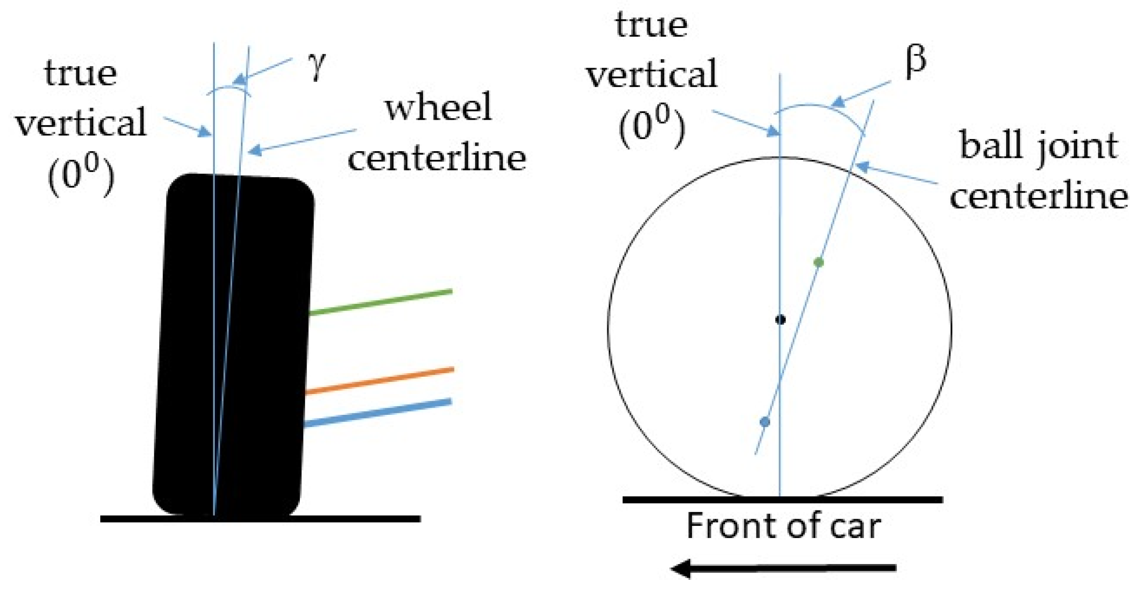
The suspension designed for a race car (rear wheel drive and front wheel steering) presented in [36] is designed from tubular components. The front axle suspension is designed from a quadrilateral mechanism with unequal arms that is linked to the chassis by ball joints. The spring and damper assembly is mounted in a quasi-horizontal position. The main disadvantage in this suspension system is the fact that it changes its dynamic behavior by changing the camber (γ) and caster (β) angles, presented in Figure 1, and wheel track during cornering. This resulted in non-linear behavior and required compensation of the steering wheel angles during cornering. At the same time, the constant change of caster angle during cornering resulted in a change of zero return (straight ahead) of the steering forces, and this induced variation in the required steering force.

Based on the above analysis of the existing solutions, the suspension system found to be the most commonly used on a Formula Student single seater (for both the front and the rear wheels/axle) was based on four-bar guiding mechanism (also called SLA—short-long arm). Compared with the regular suspension systems used by passenger cars in which the spring and damper assembly is mounted vertical (usually between the upper suspension arm and the chassis, as shown in Figure 2a), in the case of the single-seater race cars, the spring and damper assembly was mounted horizontally (Figure 2b), and this would help with force distribution and keep the chassis as low as possible. It is important to mention that both suspension systems presented in Figure 2 had a single degree of mobility (i.e., the wheel vertical travel—Y_K).

The suspension system shown in Figure 2b imposed the use of a pushrod and rocker assembly that transferred the vertical movement from the wheel to a horizontal movement to the spring and damper assembly. The rocker assembly was linked to the pushrod and the damper assembly. This allowed for the reduction of the force that the wheel transferred to the spring and damper assembly by changing the length of the rocker arms and angles, creating the opportunity to use a smaller spring and damper assembly.

Such a solution could confer the following benefits: It could decrease the variation of the camber angle, it would need a small space to be fitted, and it could accommodate tuning for both road wheel toe angle and camber angle. On the other hand, as a main disadvantage, it is well known that the four-bar suspension mechanism has contradictory behavior regarding the wheel track and camber angle variations (decrease of one of these variations generates the increase of the other one).

Starting from the classic four-bar suspension mechanism, a possible solution to avoid the above-mentioned issue is to transform the passive (pure mechanical) suspension into an active (controlled) one, and this could be achieved with the solution shown in Figure 3. In this regard, a linear actuator type assembly was disposed between the chassis and the suspension. In this way, a three-contour mechanism with two degrees of freedom (the wheel travel and the actuator movement—expansion or compression, by case) was obtained, which helped in minimizing the wheel track variation.

Besides the wheel track variation reduction, the active system had the advantage that it could change its ride height according to the weight of the vehicle and the dynamic loads that appeared during braking, accelerating, and cornering. The active suspension system behavior was mainly based on the sensors that had to read the road ahead and prepare the damping and spring stiffness for the upcoming irregularities in the rolling surface so that the driver (and the passengers as well) would feel as little as possible in the cockpit [37,38]. At the same time, this kind of suspension offers the possibility of having an equal weight distribution on the ground.

The main disadvantage of the active suspension system is the size and the complex (and expensive as well) electronical system. The risk of an error in the electronical system or misbehavior of the system, as well as the low-cost efficiency, mean the active suspension system is not one that can be fitted in a Formula Student single seater.

2. Conceptual Design of the Single-Seater Suspension System

The development of the conceptual solution for the suspension system of the single-seater race car was based on the functional particularities (including advantages and disadvantages) of the classic suspension based on the four-bar mechanism, both in the passive (Figure 2) and active version (Figure 3). The principle behind this was to define a system with a single degree of mobility (DOM = 1)—as the passive system, which could achieve adjustments specific to the mechanism with two degrees of mobility (DOM = 2)—as the active system (considering the systems in a planar configuration, as are the representations in Figure 2 and Figure 3).

The solution of the above-mentioned system was based on a five-bar mechanism that had two degrees of mobility. The initially developed suspension system, which integrated the specific pushrod-rocker assembly that helped mount the spring and damper assembly in a horizontal plane (as shown in Figure 2b) is presented in Figure 4. This would make it possible to decouple the contradictory movements (wheel track and camber angle variations) from influencing each other. The control of the second degree of mobility (with the purpose to cancel, by case, the wheel track variation or the camber angle variation) could be achieved by an actuating element (resulting in an active suspension) or by a mechanical element (passive suspension).

Thus, the active suspension could be constituted, for example, by using a linear actuator, disposed between the upper connecting rod (upper control arm as per Figure 2) of the five-bar mechanism and the chassis, with the corresponding scheme shown in Figure 5.

With the view to obtain a pure mechanical (passive) suspension able to provide the functional parameters (behavior) of the active suspension, an original design algorithm was developed, which was based on the following steps:

• In the five-bar suspension mechanism (Figure 4), the variation of the camber angle was canceled by means of a kinematic constraint of form Δγ = γ − γ₀ = 0, where γ is the current value of the camber angle, and γ₀ is the initial value;
• Performing the kinematic analysis of the suspension mechanism by imposing the vertical travel of the wheel with the help of a kinematic restriction;
• Obtaining the trajectory of a specific point on the upper rod of the five-bar mechanism; the trajectories of several points on the upper rod could be monitored, finally choosing the point that would generate a more convenient trajectory (it could be a semicircle for the planar variant of mechanism, or a hemisphere for the spatial variant);
• Replacing the kinematic restriction from step “1” with one of the following variants:

  4.1.

  Geometrical constraint roller-guide type (Figure 6), where the roller would be mounted on the upper rod, while the guide of which would attached to the chassis would have the shape defined by the trajectory obtained in step “3”;

  4.2.

  Second rocker mounted between the upper rod and the chassis (Figure 7), linked to the upper arm in the point (M) that describes the trajectory from step “3” and to the chassis at the geometrical center (M₀) of the trajectory.

Both purely mechanical solutions obtained in step “4” led to mono-mobile (DOM = 1) mechanisms (in the planar versions), and could be used on a single-seater racing car suspension as they are reduced in size, lighter, and are not as complex as an active suspension system.

It should be noted that the mechanism obtained by the second variant in step “4” (Figure 7) would be viable if the trajectory defined by the interest point (M) from the upper arm approximated a semicircle or a hemisphere. In these terms, the study continued with the determination of the global coordinates of the center point (M₀) defined on the chassis, a subject approached in “Section 4” of the work by an original synthesis method.

As mentioned, the above approach was specific to planar (2D) variants of suspension mechanisms, with a view to simplify the formulation and related schemes. Obviously, in practice, as well as in the study developed in the next sections of this paper, the spatial (3D) variant of the guiding mechanism is addressed/implemented.

Compared with the planar variants, the corresponding spatial configurations of suspension systems had one supplementary degree of mobility that was the caster angle variation. In this case, in step “1” from the above presented design algorithm, two kinematic restrictions had to be used: The one already used for the camber angle (Δγ = γ − γ₀ = 0), and a similar one for the caster angle (Δβ = β − β₀ = 0), which at step “4” was replaced through the solutions, as shown in Figure 6 and Figure 7.

Under these terms, for a better understanding of the design algorithm of the proposed suspension mechanism, Figure 8 shows the corresponding optimization flowchart. In Figure 8, ΔE is the wheel track variation, ΔL is the wheelbase variation, and Δδ is the bump steer variation.

3. The Kinematic Optimization of the Suspension Mechanism

The kinematic optimization was carried out by considering the bi-contour mechanism, as shown in Figure 9, which was obtained from the spatial variant of a five-bar suspension mechanism (whose planar scheme is that shown in Figure 4) to which the toe link (6) was added for both the front and rear axles. The resulting suspension system had three active degrees of mobility, and another two passives (the rotation of links “3” and “6” around their own axes). The passive rotations could be canceled by adding additional kinematic constraints: φ₃ = 0, φ₆ = 0.

When the car moves, the vertical travel (up–down) of the wheel determines the modification of the suspension mechanism configuration, which generates undesirable movements, namely displacements of the wheel center along the transversal and longitudinal axes (corresponding to the wheel track and wheelbase variations), as well as modifications of the wheel axis orientation (corresponding to the toe angle, camber angle, and bump steer angle variations).

Canceling or at least minimizing these variations are objectives for kinematic optimization, given the negative effects they can have on the dynamic behavior of the car, such as depreciation of stability, increasing rolling resistance, additional stress, and wear in the system, which have been stated in many works, such as [7,13,17,18,20,30,39,40].

Therefore, the following statements were considered in the kinematic optimization of the suspension mechanism shown in Figure 9:

• The vertical movement of the wheel is an independent kinematic parameter. It is controlled by a Y_K = f(t) kinematic restriction, simulating the wheel passing over a 50-mm (±25 mm) obstacle, which is transposed in the form of a sinusoidal function, Y_K = 25·sin(t), t—time [s];
• The variations of the camber (Δγ) and caster (Δβ) angles were canceled by applying kinematic restrictions: Δγ = 0, Δβ = 0 (further, for the purpose of physical implementation, these fictive kinematic restrictions would be replaced/substituted by geometric constraints through the guiding rocker MM₀, as schematically shown in Figure 7—see “Section 4” of the work);
• The goal of the optimization was to minimize the variations of the wheel track (ΔE), wheelbase (ΔL), and bump steer angle (Δδ);
• The global coordinates (X, Y, Z) of the joints that link the suspension mechanism bars to chassis (A, B, C, D—see Figure 9) are defined as design variables for optimization, assuming that the joint locations to wheel carrier are established/given by constructive aspects (i.e., the wheel carrier geometry).

The kinematic optimization was treated separately on the front and rear wheel suspension mechanisms, using quarter-car models. The optimization of the suspension system was realized with the help of a multi-objective parametric design process, by using the MSC.ADAMS suite of software, including ADAMS/Insight, a powerful optimization software [41], and ADAMS/View, which was used to develop the multi-body system (MBS) model of the suspension system [42].

The optimization study was based on design of experiments (DOE) technique, which provided methods and tools for efficiently planning and running a series of experiments on the suspension system design and analyzing the results [41]. In what follows, a general presentation of the optimization method was made, and subsequently it was implemented for optimizing the guiding mechanisms of the front and rear wheels of the single-seater race car. The parametric design through the DOE technique was performed by following the steps indicated in reference [41].

In ADAMS/View, a design objective was defined by creating its corresponding measure (wheel track, wheelbase, and bump steer variations). For each of the three design objectives, the monitored value was the root mean square (RMS) during simulation:

$$RMS=\sqrt{\frac{v_1^2+v_2^2+v_3^2+\dots v_n^2}{n}}$$

(1)

where v₁, v₂, ..., v_n represent the successive values of the parameter of interest, depending on the number of steps (n) that the simulation takes to reach the end.

Before running the optimization algorithm, the file that contained the MBS model designed in ADAMS/View was transferred in ADAMS/Insight. The design variables (factors) and design objectives (responses) were set up after opening the saved model in ADAMS/Insight. To run the optimization process, the responses and the factors were promoted from the candidates in the inclusion list (“Promote to Inclusions” in ADAMS/Insight).

Each design objective was analyzed based on a regression function that approximated the model in such way that the error between the predicted and the measured values were minimal. For example, if we only considered two design variables, the regression functions would have the following forms:

• ▪ Linear model:

$$R=a_1\ast F_1+a_3\ast F_3+e$$

(2)

• ▪ Linear model with factors interaction:

$$R=a_1+a_2\ast F_1+a_3\ast F_2+a_4\ast F_1\ast F_2+e$$

(3)

• ▪ Quadratic model:

$$R=a_1+a_2\ast F_1+a_3\ast F_2+a_4\ast F_1\ast F_2+a_5\ast F_1^2+a_6\ast F_2^2+e$$

(4)

• ▪ Cubic model:

$$\begin{gathered} R=a_1+a_2\ast F_1+a_3\ast F_2+a_4\ast F_1\ast F_2+a_5\ast F_1^2+a_6\ast F_2^2+\dots \\ \dots +a_7\ast F_1\ast F_2^2+a_8\ast F_1^2\ast F_2+a_9\ast F_1^3+a_{10}\ast F_2^3+e \end{gathered}$$

(5)

where F₁ and F₂ were the design variables (factors), a_i—the terms coefficients, R—the system response, and e—the error (that would be minimized).

Depending on the selected DOE investigation strategy, we obtained the design space and the workspace of the experiment. The design space was a matrix that presented, in a normalized form, the combinations between the factors. Thus, the “−1” value corresponded to the minimum value of the factor, and “1” to the maximum value [41], according to the previously defined variation ranges. The effective values of the factors were seen in the workspace, along the corresponding responses.

The program ran a simulation in ADAMS/View for each trial specified in this matrix to determine the responses values. After the simulations were run, the results appeared automatically in the workspace, by filling in the response columns with numerical values. Based on these results, ADAMS/Insight automatically generated the corresponding regression function, according to the selected type of regression model. The response analysis was done by using the evaluation methods presented in reference [43].

To begin, the kinematic optimization algorithm was implemented for the front wheels’ suspension mechanism (the selected tuning strategy would then be used for the rear wheels’ suspension optimization as well). The MBS model developed in ADAMS/View for the front axle suspension system is shown in Figure 10. The lower control arm (1) was linked to the chassis in points A and B through spherical joints, the rocker (5) was linked to the chassis in point C by a revolute joint, and point D was the location of the spherical joint that linked the toe link/steering rod (6) to the steering rack. In the kinematic model of the suspension system, the steering rack was fixed, so it was rigidly connected to chassis (in other words, the steering wheel is not actuated). The global coordinates of the four points were defined as design variables for the kinematic optimization of the front suspension system, as presented in

Table 1. Front axle suspension system design variables.

	X (mm)	Y (mm)	Z (mm)
A	DV_1	DV_2	DV_3
B	DV_4	DV_5	DV_6
C	DV_7	DV_8	DV_9
D	DV_10	DV_11	DV_12

.

The initial values of the design variables are (in [mm]): DV_1 = −270.37, DV_2 = 38.5, DV_3 = 108.37, DV_4 = −193.5, DV_5 = 38.5, DV_6 = −279.43, DV_7 = −297.64, DV_8 = 214.89, DV_9 = 38.21, DV_10 = −288.5, DV_11 = 101.5, DV_12 = 135.01. For each variable, the variation domain was ±20 mm relative to the initial value.

With the purpose of identifying the DOE investigation strategy that provided the optimum results from the point of view of the regression functions accuracy, several investigation strategies were tested, namely: DOE screening (level 2)—linear—Plackett Burman; DOE screening (level 2)—linear—fractional factorial; DOE response surface—Linear—Latin hypercube; DOE response surface—interactions—D-optimal; DOE screening (level 2)—interactions—D-optimal [41]. The results thus obtained highlighted that the first 4 techniques mentioned above could be used under the condition of refining the regression models, but the DOE screening (level 2)—interactions—D-optimal strategy could be used without the need for regression refining. Therefore, the optimization study of the suspension mechanism was based on this strategy.

The regression model generated by the selected strategy allowed us to consider the interaction effects between factors, which were captured through terms in the model that consisted of products of factors, as presented in Equation (3). The D-Optimal design created a model that minimized the uncertainty of the coefficients, this being characterized by its flexibility, allowing the total number of runs in an experiment to be specified, supplementing with runs from other experiments, and indicating different levels for each factor.

Based on the fact that all the evaluation parameters fell within acceptable limits, the regression functions generated by this model were valid (accurate), without any changes. As mentioned above, the kinematic optimization purpose was to minimize the three responses, corresponding to the wheel track, wheelbase, and bump steer variations.

The algorithm used in the kinematic optimization of the suspension system was OptDes-generalized reduced gradient (GRG), provided with ADAMS/Insight, which required that factors have range limits, since it worked in scaled space [42]. This algorithm used the MinTo function, which constrained the response (goal) to be as close to the target value as possible (“0”).

The optimum values of the design variables were obtained by running the tuning to the “0” variations of the targets. These values were as follows (in [mm]): DV_1 = −230.37, DV_2 = −1.5, DV_3 = 68.37, DV_4 = −233.5, DV_5 = −1.5, DV_6 = −319.43, DV_7 = −257.64, DV_8 = 254.89, DV_9 = 78.21, DV_10 = −248.5, DV_11 = 61.5, DV_12 = 175.01.

With these values, through the kinematic analysis performed in ADAMS/View, the variations of the interest parameters for the optimal (after optimization) suspension mechanism were obtained (Figure 11, Figure 12 and Figure 13). To compare, the results corresponding to the initial mechanism (before optimization) are also presented, noting a significant improvement of all the parameters, which demonstrated the viability/usefulness of the implemented optimization algorithm.

According to the optimization flowchart shown in Figure 8, the next step after the kinematic optimization of the suspension mechanism consisted of determining the location of a point (M) on the upper control arm whose trajectory during the simulation (depending on the imposed wheel vertical travel) was close to a convenient circular or spherical one, so that later it would be easy to determine the center (M0) of this trajectory on the chassis (for notations, see the schematic planar model in Figure 7), as presented in “Section 4” of the work. In this regard, the trajectories of several points on the upper arm were monitored, finally choosing the point that generated more convenient trajectory, which had the following global coordinates (in its initial position) (in [mm]): X_M = −432.8, Y_M = 274.8, Z_M = 38. The trajectory (Γ) of this point during the kinematic analysis of the front wheel suspension mechanism, which was controlled by the kinematic restriction Y_K = 25·sin(time), can be shown in Figure 14.

For the rear wheel suspension system, the MBS model was also designed in ADAMS/View (Figure 15). The optimization purpose was, as in the case of the front wheel suspension, to minimize the wheel track, wheelbase, and bump steer variations, while the camber and caster angles variations were canceled in this stage with the help of kinematic restrictions.

As for the front suspension system, points A and B were considered as the centers of two spherical joints that link the lower control arm (1) to the chassis, point C was the link between the rocker (5) and the chassis, and point D represented the center of the spherical joint between the toe arm (6) and the chassis. The initial values of the design variables were (in [mm]): DV_1 = −341.42, DV_2 = −50.0, DV_3 = −1310.74, DV_4 = −319.62, DV_5 = −50.0, DV_6 = −1617.95, DV_7 = −344.97, DV_8 = 211.15, DV_9 = −1743.65, DV_10 = −213.76, DV_11 = 54.01, DV_12 = −1720.29 (with correlations in notations similar to those in Table 1).

As mentioned, in the rear wheel suspension optimization process, the same investigation strategy as for the front wheel suspension was used, namely DOE screening (level 2)—interactions—D-optimal. The optimization algorithm used was OptDes-GRG, with the MinTo operator. By running the optimization process, the following optimal values of the design variables were obtained (in [mm]): DV_1 = −381.42, DV_2 = −90.0, DV_3 = −1270.74, DV_4 = −279.62, DV_5 = −10.0, DV_6 = −1657.95, DV_7 = −384.97, DV_8 = 171.15, DV_9 = −1783.65, DV_10 = −173.76, DV_11 = 14.01, DV_12 = −1760.29.

Through the kinematic analysis performed in ADAMS/View, the variation diagrams shown in Figure 16, Figure 17 and Figure 18 were obtained, for the initial (before optimization) and optimal (after optimization) suspension mechanisms, observing (as in the case of the front suspension) significant reductions in the monitored parameters variations.

Further, in a similar way to those presented for the front wheel suspension, the most convenient trajectory (Γ) generated by a point (M) located on the upper arm (3) of the rear wheel suspension mechanism was selected, as shown in Figure 19, where the interest point had the following global coordinates (in the initial position) (in [mm]): X_M = −525.9, Y_M = 225.9, Z_M = −1663.8. For the chosen trajectory, the global coordinates of the center point M₀ on the chassis were determined according to the synthesis method presented in the next section of the paper.

Concluding, it was observed that with the canceling of the camber and caster angle variations (which in this stage were controlled by kinematic restrictions), the wheelbase, wheel track, and bump steer angle variations were significantly reduced, which was not possible in the case of the classic four-bar suspension mechanism. As a result of the implemented optimization procedure, the variations of all kinematic parameters were within the accepted limits for the Formula Student single seater, both for the front and rear wheels, with a positive effect on the ride and handling performance of the car.

4. Synthesis of the Proposed Solution

The innovative solution proposed in this work, for both the front and rear suspension systems, corresponded to the guiding mechanism shown schematically in Figure 7, whose spatial variant (Figure 20) enabled the minimization (even canceling) of the camber and caster angles variations by using a guiding rocker (4) mounted between the upper arm (3) and the chassis (0). The guiding rocker was arranged so as to replace/substitute the two fictive kinematic restrictions (Δγ = 0, Δβ = 0) used in the kinematic optimization depicted in the previous section of the work.

The location of the point/end M on the guiding rocker was previously determined for the initial position of the suspension mechanism (when the car was in rest), along with the trajectory of this point during the kinematic analysis (see Figure 14 and Figure 19). The problem raised by the proposed solution was the fact that we needed to determine where the focal point (M₀) of the guiding rocker was on the chassis, so that is would assure the cancelation of the camber and caster variations. To do this, in the following, we proposed a synthesis algorithm based on the method of least squares, through which, starting from the imposed movement of point M (the trajectory Γ described through a series of successive positions M_k), the global coordinates of point M₀ on the chassis (and thus the spatial arrangement of the guiding rocker) was determined.

The constraint of point M on the guiding rocker consisted in the fact that it had to be on a fixed surface or curve with point M₀ on the chassis. In the case of guiding point M on a sphere with the center in M₀ (Figure 21), the guiding (constraint) equation had the form:

$${\left({\mathrm{X}}_{\mathrm{M}}-{\mathrm{X}}_{\mathrm{M}0}\right)}^2+{\left({\mathrm{Y}}_{\mathrm{M}}-{\mathrm{Y}}_{\mathrm{M}0}\right)}^2+{\left({\mathrm{Z}}_{\mathrm{M}}-{\mathrm{Z}}_{\mathrm{M}0}\right)}^2-l_4^2=0$$

(6)

where l₄ is the length of the guiding rocker.

The point coordinates (X_M, Y_M, Z_M) in the global reference frame (attached to chassis) were input data of the synthesis problem. The coordinates of the chassis M₀ point (X_M0, Y_M0, Z_M0) and the length of the guiding rocker (l₄) were unknown and needed to be computed.

Equation (6) can be rewritten under the following form:

$${\mathrm{X}}_{\mathrm{M}}^2+{\mathrm{Y}}_{\mathrm{M}}^2+{\mathrm{Z}}_{\mathrm{M}}^2+{\mathrm{X}\ast \mathrm{X}}_{\mathrm{M}}+{\mathrm{Y}\ast \mathrm{Y}}_{\mathrm{M}}+{\mathrm{Z}\ast \mathrm{Z}}_{\mathrm{M}}+\mathrm{R}=0$$

(7)

where: $\mathrm{X}=-2{\ast \mathrm{X}}_{\mathrm{M}0}, \mathrm{Y}=-2{\ast \mathrm{Y}}_{\mathrm{M}0}, \mathrm{Z}=-2{\ast \mathrm{Z}}_{\mathrm{M}0}, \mathrm{R}={\mathrm{X}}_{\mathrm{M}0}^2+{\mathrm{Y}}_{\mathrm{M}0}^2+{\mathrm{Z}}_{\mathrm{M}0}^2-{\mathrm{l}}_4^2$.

Rewriting Equation (7) for the “m” number of positions that could be imposed to the wheel and subtracting the first equation, “m − 1” equations with 3 unknown (X, Y, Z) were obtained:

X·[(X_M)_k+1 − (X_M)₁] + Y·[(Y_M)_k+1 − (Y_M)₁] + Z·[(Z_M)_k+1 − (Z_M)₁] = (r)₁ − (r)_k+1

(8)

where ${\left(\mathrm{r}\right)}_{\mathrm{k}}={\left({\mathrm{X}}_{\mathrm{M}}^2+{\mathrm{Y}}_{\mathrm{M}}^2+{\mathrm{Z}}_{\mathrm{M}}^2\right)}_{\mathrm{k}}$, which leads to a function of form:

F_k (X, Y, Z) = L_k, k = 1... m − 1.

(9)

For m = 4 imposed positions, the system (4) was a linear one, with 3 equations and 3 unknowns. However, as there had to be more than 3 imposed finite positions, we obtained an over-determined system that could be solved by means of the least squares approach.

If X’, Y’, Z’ were a set of values that could be verified with approximation of one part of the Equation (9), for example, the solution of the system formed by the first 3 equations, would result:

F_k (X’, Y’, Z’) = L’_k, k = 1... m − 1.

(10)

Subtracting the Equation (10) from (9) we obtain:

F_k (X, Y, Z) − F_k (X’, Y’, Z’) = L_k − L’_k = d_k

(11)

Assuming that the differences δx = X − X’, δy = Y − Y’, δz = Z − Z’ were small enough as in the developed functions F_k based on the Taylor formula, we could neglect the higher-order terms, and the equation system (11), with its unknown δx, δy, δz, would be:

a_k· δ_x + b_k· δ_y + c_k· δ_z = d_k

(12)

where a_k = (X_M)_k+1 − (X_M)₁, b_k = (Y_M)_k+1 − (Y_M)₁, c_k = (Z_M)_k+1 − (Z_M)₁.

According to the method of least squares, the best solutions of the system (12) were those values δx, δy, δz for which the objective function:

$$\mathrm{f}\left({\mathsf{\delta }}_{\mathrm{X}},{\mathsf{\delta }}_{\mathrm{Y}},{\mathsf{\delta }}_{\mathrm{Z}}\right)={\displaystyle \sum }_{\mathrm{k}=0}^{\mathrm{m}-1}{({\mathrm{a}}_{\mathrm{k}}{\ast \mathsf{\delta }}_{\mathrm{X}}+{\mathrm{b}}_{\mathrm{k}}{\ast \mathsf{\delta }}_{\mathrm{Y}}+{\mathrm{C}}_{\mathrm{k}}{\ast \mathsf{\delta }}_{\mathrm{Z}}-{\mathrm{d}}_{\mathrm{k}})}^2$$

(13)

is minimal, meaning:

$$\frac{\mathsf{\delta }\mathrm{f}}{\delta {\mathsf{\delta }}_x}=0,\frac{\mathsf{\delta }\mathrm{f}}{\delta {\mathsf{\delta }}_y}=0,\frac{\mathsf{\delta }\mathrm{f}}{\delta {\mathsf{\delta }}_z}=0$$

(14)

Thus, a linear system of 3 equations with 3 unknowns (δx, δy, δz) is obtained:

[aa] · δ_x + [ab] · δ_y + [ac] · δ_z = [ad],
[ba] · δ_x + [bb] · δ_y + [bc] · δ_z = [bd],
[ca] · δ_x + [cb] · δ_y + [cc] · δ_z = [cd],

(15)

where $\left[aa\right]={\displaystyle \sum }_{k=1}^{m-1}{a}_k^2, \left[ab\right]={\displaystyle \sum }_{k=1}^{m-1}{a}_k\ast b_k,$ and so on.

The best approximate solution of the system (15) is:

X = X’ + δx, Y = Y’ + δy, Z = Z’ + δz,

(16)

$${\mathrm{X}}_{\mathrm{M}0}=-\frac{\mathrm{X}}{2}{\ast \mathrm{Y}}_{\mathrm{M}0}=-\frac{\mathrm{Y}}{2}{\ast \mathrm{Z}}_{\mathrm{M}0}=-\frac{\mathrm{Z}}{2}$$

(17)

The average quadratic errors with which the solutions were calculated are:

$${\mu }_X=\epsilon \ast \sqrt{\frac{∆A}{∆}}, {\mu }_Y=\epsilon \ast \sqrt{\frac{∆B}{∆}}, {\mu }_Z=\epsilon \ast \sqrt{\frac{∆C}{∆}},$$

(18)

where Δ is the determinant of the system (15); ΔA, ΔB, and ΔC are algebraic coefficients of the [aa], [bb], and [cc] elements from the main diagonal, and ε is the error with which d_k was computed:

$$\epsilon =\frac{\sqrt{{{\displaystyle \sum }}_{k=1}^{m-1}{\left(a_k\ast {\mathsf{\delta }}_X+b_k\ast {\mathsf{\delta }}_Y+c_k\ast {\mathsf{\delta }}_Z-d_k\right)}^2}}{m-4},$$

(19)

The sphere radius (i.e., the guiding rocker length) could be now determined from the equation:

$$l_4=\sqrt{{\left({\mathrm{X}}_{\mathrm{M}}-{\mathrm{X}}_{\mathrm{M}0}\right)}^2+{\left({\mathrm{Y}}_{\mathrm{M}}-{\mathrm{Y}}_{\mathrm{M}0}\right)}^2+{\left({\mathrm{Z}}_{\mathrm{M}}-{\mathrm{Z}}_{\mathrm{M}0}\right)}^2}$$

(20)

In the particular case where the point M is moving on a circle with its center in M₀ on the chassis, meaning that the guiding rocker MM₀ would have two spherical joints on the chassis (M₀′, M₀”), the geometrical place of the M point would be on a circle Γ (Figure 22), which could be determined by intersecting the sphere S, defined by the Equation (6), with the π plane, with the following equation:

$$\left({\mathrm{X}}_{\mathrm{M}}-{\mathrm{X}}_{\mathrm{N}}\right)\ast \cos \mathsf{\alpha }+\left({\mathrm{Y}}_{\mathrm{M}}-{\mathrm{Y}}_{\mathrm{N}}\right)\ast \cos \mathsf{\beta }+\left({\mathrm{Z}}_{\mathrm{M}}-{\mathrm{Z}}_{\mathrm{N}}\right)\ast \cos \mathsf{\eta }=0$$

(21)

where N is a point belonging to the plane, and cos α, cos β, and cos η are the cosines of the axis normal to the plane (i.e., the rotation axis).

Equation (21) can be rewritten as:

$${\mathrm{X}}_{\mathrm{M}}+{\mathrm{r}}_1·{\mathrm{Y}}_{\mathrm{M}}+{\mathrm{r}}_2+{\mathrm{Z}}_{\mathrm{M}}+{\mathrm{r}}_3=0$$

(22)

where r₁, r₂, and r₃ are given from the following equations:

$$r_1=\frac{\cos \beta }{\cos \alpha },r_2=\frac{\cos \eta }{\cos \alpha }, r_3=-\left(X_N+r_1·Y_N+r_2·Z_N\right)$$

(23)

For an “m” number of finite positions of the point M, by subtracting the first equation (corresponding to the initial position) from the others, the Equation (22) becomes:

$$\left[{\left(X_M\right)}_{k+1}-{\left(X_M\right)}_1\right]+r_1\ast \left[{\left(Y_M\right)}_{k+1}-{\left(Y_M\right)}_1\right]+r_2\ast \left[{\left(Z_M\right)}_{k+1}-{\left(Z_M\right)}_1\right]=0, k=1,\dots m-1$$

(24)

Equation (6) was used to determine the location of M₀ according to the algorithm for determining the center of a spherical surface. The orientation of the revolute joint axis (M_0′–M_0”) was obtained by (24), which had a similar solution as (8).

The presented algorithm was transposed in a computer program by using MATLAB. The actual numerical implementation was reflected in the global coordinates of the points M₀ in which the guiding rocker was connected to the chassis, along with an additional point M_0′ by which the revolute joint axis of the rocker was defined, as follows:

• The front wheel suspension mechanism (Figure 23): X_M0 = −323.9, Y_M0 = 245.9, Z_M0 = 42.9; X_M0′ = −318.2, Y_M0′ = 250.4, Z_M0′ = −56.8 (in mm);
• The rear wheel suspension mechanism (Figure 24): X_M0 = −282.1, Y_M0 = 152.4, Z_M0 = −1698.3; X_M0′ = −267.5, Y_M0′ = 154.4, Z_M0′ = −1599.4 (in mm).

By the kinematic analysis of the proposed front and rear suspension mechanisms, approximately zero variations of the camber and caster angles were obtained. In addition, the variations of the wheelbase, wheel track, and bump steer angle for the suspension mechanisms with the guiding rocker shown in Figure 23 and Figure 24 were very close to those corresponding to the five-bar mechanism-based suspension systems (the optimal curves in Figure 11, Figure 12 and Figure 13, and, respectively, Figure 16, Figure 17 and Figure 18). These very good correlations between results demonstrate the viability of replacing the fictive kinematic restrictions (by which the variations of the camber and caster angles were initially canceled) by the physical geometrical constraints associated with the guiding rockers.

As mentioned, most Formula Student race cars use the double wishbone (four-bar) suspension mechanism (schematically represented in Figure 2b). This solution was also implemented on the initial race car developed at Transilvania University of Brasov (Brasov, Romania, BlueStreamline), on both the front and the rear axles, with which the single seater obtained good results in the competitions where it participated (on the circuits from Silverstone, Catalunya, and Varano). Prior to implementation, that double wishbone suspension was kinematically optimized by an algorithm based on DOE techniques and linear regression functions, as presented in previous authors’ papers [31,32]. The proposed suspension system solution is an improvement of the classical double wishbone suspension system, by being able to decouple the mentioned contradictory kinematic variations (the issues in which the double wishbone suspension mechanism was deficient), thus improving the dynamic behavior of the suspension (car, in general).

The values of several important characteristics, when the car was in static rest, of the two suspension systems implemented/used on the Formula Student single-seater race car developed at Transilvania University of Brasov (the classical four-bar mechanism, and the new solution depicted in this work) are shown in

Table 2. Suspension system characteristics.

	Four-Bar	New Solution	Four-Bar	New Solution
	Front		Rear
Roll center height [mm]	250	246	280	290
Caster center height [mm]	150	147	190	188
Anti-dive/squat [%]	50	49	65	67
Camber [deg]	1.5		1
Toe [deg]	0.7		0.5
Kingpin angle [deg]	−3.9		−4.07
Steering axis offset [mm]	3.1		0
Scrub radius [mm]	30.75		2
Caster trail [mm]	17.25		8
Track width at wheel center [mm]	1210		1150

. It is well known that the static characteristics of any suspension system are given by the wheel position in space (camber angle, toe angle, track width at wheel center) and by the wheel carrier ball joint positions (kingpin angle, steering axis offset, scrub radius, caster trail). The static parameters were carried over from the initially tuned four-bar suspension system, and as the optimization process of the new (proposed) solution was based by moving the hard points that connect the suspension system to the chassis and the wheel carrier hard points were not affected by this, the static suspension system metrics did not change relative to the classical four-bar suspension.

5. Development and Testing of the Physical (Experimental) Prototype

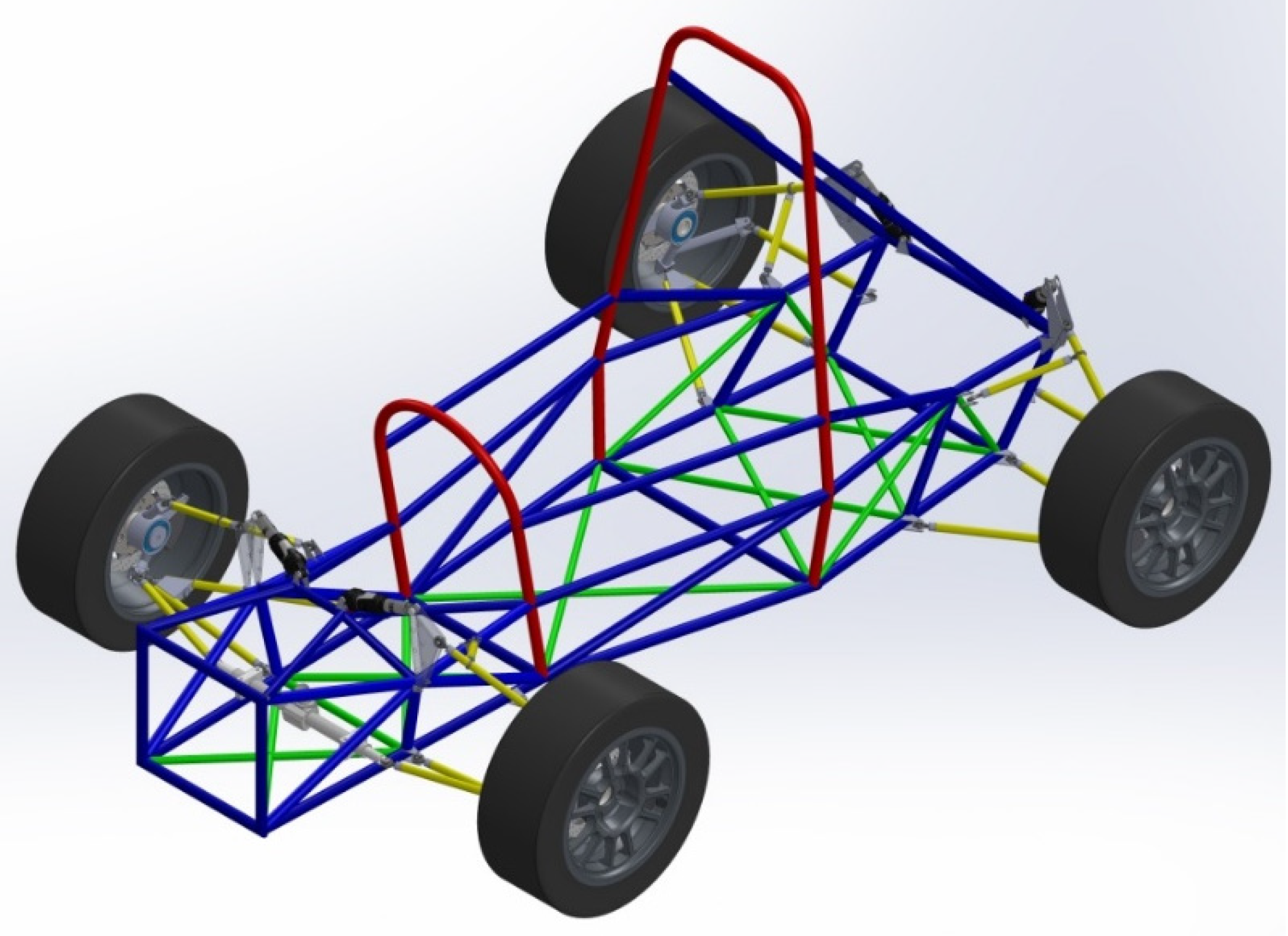
The process of modeling, simulation, and optimization in a virtual environment, the results of which are presented in Figure 25 in the form of the full-vehicle virtual prototype, preceded the implementation of the physical prototype, a subject addressed from here on. In order to develop the physical prototype, the following steps were taken: Embodiment design of the full-vehicle suspension system, starting from which the execution and assembly drawings were generated; executing or acquisitioning the components; assembling the components; acquisitioning and mounting the data monitoring system (sensors).

The physical prototype of the proposed suspension system was implemented and tested with the help of BlueStreamline, the Formula Student team of the Transilvania University of Brașov (Figure 26). The data acquisition system used to measure damper travel consisted of two short distance sensors (sharp), an Arduino MEGA 2560 development board, a breadboard, and a SD memory card socket. The programming language used by the microcontroller was C#. The data acquisition system used to measure the forces transmitted in the chassis consists of an AQ-1 data logger, which had a built-in force sensor that was mounted on the chassis near its center of mass. The data thus collected were transferred for postprocessing into EXCEL.

In order to evaluate the dynamic behavior of the single-seater prototype, several tests were carried out, which were similar to those the single seater would have to pass through in the competitions. Further, the results obtained in the case of the left–right cornering and passing over vibrators, as well as a skid pad type event, were presented. The tests were performed on the karting circuit from Prejmer (Figure 27). For the overpass vibrators’ test, all the corresponding vibrators of all corners must be reached. This test aimed to check the speed response (reaction) of the suspension system (Figure 28), and the way it supports lateral forces (Figure 29).

According to the diagrams shown in Figure 29, it is possible to observe the shift of loading forces that act on the car from on one side to the other (left–right) at the time of turning, in both wide and tight corners. At the same time, a linear behavior was observed in the suspension system, which induced a good handling of the car and reduced the necessary corrections in the steering wheel while turning.

The skid pad type event was carried out in an especially arranged track that mimicked the Formula Student layout shown in Figure 30. The diagrams in Figure 31 show the movement of the front axle spring and damper assembly during constant cornering (left and right). By analyzing the results from Figure 31 (maximum damper travel of +/−20 mm) and Figure 28 (maximum damper travel of +/−30 mm), it is clearly seen that the suspension did not reach its end stops during the skid pad event. On the other hand, by correlating the lateral force diagram presented in Figure 32 with the circuit layout shown in Figure 30, it is clear that the suspension had a linear behavior that was easy to anticipate from a driver point of view.

Furthermore, as the bump steer variation was reduced to zero it was easy to deduce that the only toe angle that the front wheels had was the input given by the driver from the steering wheel, and the rear toe angle was equal to the static toe angle (0.5°). As the bump camber and bump caster variations were reduced to zero as well, the camber and caster angles during cornering would be equal to the static ones (1.5° front and 1° on the rear camber, and −3.9° front and −4.07° rear on the caster angle).

Based on the results of the spring and damper assembly movement presented in Figure 28 and Figure 31, it is clear that the race car had a linear all-around behavior and had good handling capabilities. As this is a race car, we did not test or look at any ride metrics; nor did we aim to tune any of them. In any race car, the handling metrics are more important than the ride metrics, as the ride is influenced by several components that the given suspension system does not have, such as suspension bushes and anti-roll bars, and any attempt to tune them could be made only by changing the damping or spring characteristics, and the presented paper did not aim to tune for them.

6. Conclusions

While for passenger cars there are a multitude of suspension system solutions, in the case of single-seater race cars, due to the specific regulations, the range of solutions is limited, most of the existing solutions being based on the classical four-bar suspension mechanism, which has the major disadvantage of the contradiction between the wheel track and the camber angle variations.

For reasons of complexity, maintenance, and cost, it is preferable to use a purely mechanical suspension system, although the active suspension would ensure a superior behavior. The proposed suspension system offered the advantages of the purely mechanical suspension; while functional, it was close to the behavior of the active suspension, and could be implemented on both the front and rear axles of the single seater (no matter which of them is motor axle).

The design, simulation, and optimization process in a virtual prototyping environment is aimed at evaluating and improving the kinematic behavior/movement of the suspension system, which directly affect vehicle ride and handling performance. The optimization study was based on a DOE screening—interactions—D-optimal investigation strategy, and it resulted in a significant improvement of the measured target variations by only requiring minor changes to the initial setup of the system (front or rear).

Based on the suspension performance shown in Figure 28 and Figure 31 and the chassis lateral forces presented in Figure 29 and Figure 32, both the suspension optimization viability and suspension system performance could be acknowledged for various road conditions on which the experimental data recordings were performed, such as straight line, corners, and bumps (vibrators). A linear suspension behavior was obtained, without sudden changes (which could induce a non-linear behavior of the single seater).

The single-seater race car that was equipped with the suspension system depicted in this work managed to pass all the Formula Student tests, and thus was able to participate in any Formula Student competition, thus proving the integrity of the tuning strategy, and the high performance of the proposed suspension system.