Featured Application
This paper provides a fast and accurate method to identify the frequency-dependent rotordynamic coefficients of annular seals.
Abstract
The elliptical orbit whirl model is widely used to identify the frequency-dependent rotordynamic coefficients of annular seals. The existing solution technique of an elliptical orbit whirl model is the transient computational fluid dynamics (CFD) method. Its computational time is very long. For rapid computation, this paper proposes the orbit decomposition method. The elliptical whirl orbit is decomposed into the forward and backward circular whirl orbits. Under small perturbation circumstances, the fluid-induced forces of the elliptical orbit model can be obtained by the linear superposition of the fluid-induced forces arising from the two decomposed circular orbit models. Due to that the fluid-induced forces of circular orbit, the model can be calculated with the steady CFD method, and the transient computations can be replaced with steady ones when calculating the elliptical orbit whirl model. The computational time is significantly reduced. To validate the present method, its rotordynamic results are compared with those of the transient CFD method and experimental data. Comparisons show that the present method can accurately calculate the rotordynamic coefficients. Elliptical orbit parameter analysis reveals that the present method is valid when the whirl amplitude is less than 20% of seal clearance. The effect of ellipticity on rotordynamic coefficients can be ignored.
1. Introduction
Annular seals are widely used in turbomachinery to control the leakage flow through rotor–stator clearances from high-pressure regions to low-pressure regions [1,2]. Besides leakage flow reduction, annular seals are intended to serve as vibration damping devices. However, the flow in seals often generates fluid-induced forces that can destabilize the rotor [3,4]. As modern turbomachinery is moving towards higher operating parameters, the fluid-induced forces and their influence on the rotordynamic stability are becoming more pronounced [5,6]. Accurate and fast identification of the rotordynamic coefficients is essential in the seal design and evaluation process.
For small orbital motion of the rotor about the stator center, four forces are generated, Frr, Frθ, Ftr, and Ftθ, as shown in Figure 1. For the four forces, the first subscript represents the force direction, where “r” means that the force is in the displacement direction, and “t” means that the force is perpendicular to the displacement direction. The second subscript represents the disturbance parameter, where “r” represents the displacement disturbance, and “θ” represents the whirl velocity disturbance.
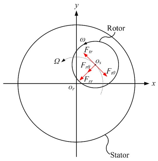
Figure 1.
Fluid-induced forces acting on the whirl rotor.
A rotor displacement disturbance produces two forces. One force is Frr, which is in the displacement direction. The other force is Ftr, which is perpendicular to the displacement direction. The two forces are proportional to the rotor displacement (whirl orbit radius r). The force Frr is divided by the rotor displacement r to yield the direct stiffness K. The force Ftr is divided by the rotor displacement r to yield the cross-coupled stiffness k.
The rotor whirl velocity disturbance also produces two forces. One force is Ftθ, which is perpendicular to the displacement direction. The other force is Frθ, which is in the displacement direction. The two forces are proportional to the rotor whirl velocity. The force Ftθ is divided by the rotor whirl velocity Ωr to yield the direct damping C. The force Frθ is divided by the rotor whirl velocity Ωr to yield the cross-coupled damping c.
The methods for rotordynamic coefficient identification of annular seals can be grouped into the analytical method based on bulk-flow theory [7] and the numerical method based on computational fluid dynamics (CFD) simulation [6]. The bulk-flow method was developed in the early 1980s. This method permits quick calculations with some simplifying assumptions. The one-control volume model is the simplest one [8]. Each seal cavity is represented with one control volume. Variations in pressure, velocity, and density in the control volume are neglected. The average values of variables are used. Considering that the jet flow region and vortex flow region have different flow patterns, the two-control volume model was developed by Wyssmann et al. [9] in 1984. Each seal cavity is divided into two parts. In 1991, the three-control volume model was developed to take into account the jet flow beneath the seal tooth [10]. All these control volume models use friction factor corrections to link the wall stress with average flow velocity [8,9,10]. The numerical accuracy of the bulk-flow model largely relies on these corrections [11,12]. In practice, it is hard to accurately model/prescribe these corrections, because they change with seal geometries and operating conditions.
From the one-control volume model to three-control volume model, the description of the seal flow field becomes more detailed. When a large number of control volumes are employed to fill the seal flow domain, the analysis results tend to reach the real flow field. This led to the development of the CFD method [13]. With the progress of computer technologies, the CFD method has received increased attention since the 1990s. The seal flow domain is discretized by numerous grid cells. The complete Navier–Stokes equations are solved. The prediction capability and accuracy are improved. The CFD method can be classified either as steady [14] or transient [15]. The steady CFD method assumes that the rotor performs a circular orbit whirl around the stator center. The unsteady problem can be transformed into a steady one by solving the three-dimensional flow field in the frame of reference attached to the whirling rotor [13]. Curve-fitting technologies are subsequently employed to identify the rotordynamic coefficients [13]. With this method, the obtained rotordynamic coefficients are frequency independent [13,14]. The latest research results show that many annular seals possess frequency-dependent rotordynamic coefficients, including the labyrinth seal [16,17], pocket damper seal [17], hole-pattern seal [18,19], etc. Interaction between the acoustic waves in a circumferential annulus and the rotor excitation frequency is the cause of the frequency dependency [20].
To identify the frequency-dependent rotordynamic coefficients of annular seals, the transient CFD method is applied. The transient CFD method directly solves the unsteady flow field with a mesh deformation technique. The rotor performs the periodic motion. The time-dependent fluid-induced forces are obtained to identify the frequency-dependent rotordynamic coefficients. According to the difference in whirl orbit, the transient CFD method can be divided into a linear orbit model [21], circular orbit model [22], and elliptical orbit model [23]. In 2007, Chochua et al. [21] employed the linear orbit model to determine the frequency-dependent rotordynamic coefficients of a hole-pattern seal. The rotor was given a periodic motion in one direction. The frequency-dependent rotordynamic coefficients can be obtained with one transient computation for each frequency. Subsequently, Yan et al. [22] advanced Chochua et al.’s model by applying the circular orbit model in 2011. Motion in two orthogonal directions was imposed on the rotor. The amplitudes in two orthogonal directions were equal. The results showed that the circular orbit model has a superior accuracy to the linear orbit model. However, the circular orbit model is more time-consuming because two transient computations of the forward and backward whirls are required for each frequency. Considering the computational time, the elliptical orbit model was applied by Yan et al. [23] in 2012. Compared with the circular orbit model, the consumed time was reduced by 50% because one transient computation was required for each frequency. The accuracy of the elliptical orbit model was equivalently high. In addition, the elliptical orbit model is more representative of the real rotor excitation. The elliptical orbit model is widely used to predict the frequency-dependent rotordynamic coefficients of annular seals [24,25,26].
Although a significant reduction of computational time has been achieved by the elliptical orbit model, the computational cost is still high because of transient computations [23]. In this paper, the orbit decomposition method is proposed to reduce the computational time. The elliptical whirl orbit is decomposed into the forward and backward circular whirl orbits. Under small perturbation circumstances, the rotordynamic problem can be linearized. The fluid-induced forces of the elliptical orbit model can be obtained by the linear superposition of the fluid-induced forces arising from the two decomposed circular orbit models. As the fluid-induced forces of the circular orbit model can be calculated with the steady CFD method, the transient computations can be replaced with the steady ones in the solution process of the elliptical orbit whirl model. The computational time is largely reduced. To validate the orbit decomposition method, its rotordynamic results are compared with those of the transient CFD method and experimental data. To study the effects of elliptical orbit parameters on the results of the present method, two major parameters are investigated, whirl amplitude and ellipticity.
2. Review of Transient Method for Rotordynamic Coefficient Identification
Before going into the details of the orbit decomposition method for rotordynamic coefficient identification, it is necessary to introduce the traditional transient method. Figure 2 shows the elliptical orbit whirl model. The rotor performs an elliptical orbit whirl at a speed of Ω around the stator center os, and rotates about its own axis at a speed of ω. This whirl orbit is expressed as:
where X and Y are the x and y direction rotor displacements, respectively, Ω is the rotor whirl velocity, t is the time, α is the ellipse attitude angle, and a and b are the major semiaxis and minor semiaxis, respectively.
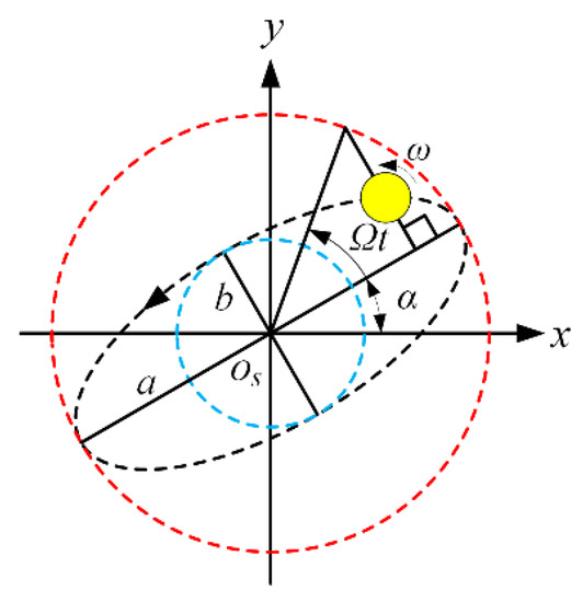
Figure 2.
Elliptical orbit whirl model. The blue circle and red circle are auxiliary circles that help to locate the position of the whirl rotor. The diameter of the red circle is the major axis of the ellipse, and the diameter of the blue circle is the minor axis of the ellipse.
As the rotor location and fluid domain change with time, transient analysis and the moving mesh technique are required. A whirl period is divided into multiple time steps. The three-dimensional unsteady flow field is calculated step by step. In general, the transient computation should be run for several whirl cycles until the accurate transient solution is reached. The transient analysis is very time-consuming.
After the time-dependent fluid-induced forces are obtained, the rotordynamic coefficients can be determined. For small orbital motion of the rotor about the stator center, the fluid-induced forces are quantified by specifying a set of linearized rotordynamic coefficients, as shown in the following equation [23]:
where (Fx, Fy) are the x and y direction components of the fluid-induced force acting on the rotor, and (K, k) and (C, c) are the stiffness and damping coefficients, respectively. All the coefficients are functions of rotor whirl velocity Ω.
Substituting Equation (1) into Equation (2), the force–displacement relation of the elliptical orbit model is expressed as:
For each whirl frequency, the cases of Ωt = 0 rad and Ωt = π/2 rad are selected to identify the frequency-dependent rotordynamic coefficients. Substituting Ωt = 0 rad into Equation (3), the force–displacement relation is expressed as:
where (, ) are the x and y direction fluid-induced force components of the elliptical orbit model in the case of Ωt = 0 rad.
Substituting Ωt = π/2 rad into Equation (3), the force–displacement relation is expressed as:
where (, ) are the x and y direction fluid-induced force components of the elliptical orbit model in the case of Ωt = π/2 rad.
From Equations (4) and (5), the frequency-dependent rotordynamic coefficients can be obtained as:
3. Rotordynamic Coefficient Identification Based on Orbit Decomposition Method
The orbit decomposition method is established for the rapid identification of frequency-dependent rotordynamic coefficients for annular seals. This method includes three parts: elliptical orbit decomposition, fluid-induced force superposition, and rotordynamic coefficient identification. The detailed identification procedures of frequency-dependent rotordynamic coefficients are shown in Figure 3.
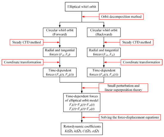
Figure 3.
Rotordynamic coefficient identification procedures of orbit decomposition method.
3.1. Elliptical Orbit Decomposition
Equation (1) gives the mathematical expression of the elliptical whirl orbit. It can be rearranged as:
Equation (7) shows that the elliptical whirl orbit can be decomposed into two circular whirl orbits. One is whirling in the same direction as the rotor’s spin direction (forward) and the other is whirling opposite to the shaft rotation (backward). Figure 4 shows this decomposition and this decomposition is defined as:
where (Xf, Yf) are the x and y direction rotor displacements of the forward circular orbit whirl model, and (Xb, Yb) are the x and y direction rotor displacements of the backward circular orbit whirl model.
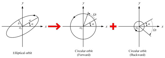
Figure 4.
Elliptical Orbit Decomposition.
3.2. Fluid-Induced Force Superposition
Substituting Equation (8) into Equation (2), the fluid-induced forces (Fx, Fy) of the elliptical orbit model are obtained as:
For the forward circular orbit whirl model, the fluid-induced forces (Fxf, Fyf) are expressed as:
For the backward circular orbit whirl model, the fluid-induced forces (Fxb, Fyb) are expressed as:
Hence, the fluid-induced forces of the elliptical orbit model can be obtained by the superposition of fluid-induced forces due to the forward and backward circular orbit whirl models, as shown in Figure 5. The fluid-induced forces of the elliptical orbit model can be obtained by:
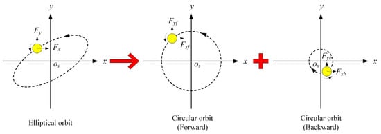
Figure 5.
Fluid-induced force superposition based on orbit decomposition method.
In Figure 5 and Equation (12), the fluid-induced forces Fx and Fy are positive when they are in the positive directions of the x-axis and y-axis, respectively. Conversely the fluid-induced forces Fx and Fy are negative when they are in the negative directions of the x-axis and y-axis, respectively.
For the circular orbit model, the tangential force Ft and radial force Fr acting on the rotor are constant at any circumferential position. According to the coordinate transformation shown in Figure 6, the time-dependent fluid-induced forces of the two decomposed circular orbit models can be expressed as:
and
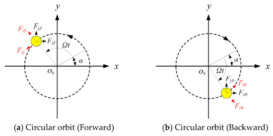
Figure 6.
Coordinate transformation of fluid-induced forces.
In Figure 6 and Equations (13) and (14), the tangential force Ft and radial forces Fr are positive when they are in the same directions as the forward whirl and radial displacement, respectively. Conversely, the tangential force Ft and radial forces Fr are negative when they are in the opposite directions of the forward whirl and radial displacement, respectively.
Substituting Equations (13) and (14) into Equation (12), the time-dependent fluid-induced forces of the elliptical orbit model can be calculated as:
For the circular orbit whirl model, the rotor whirls at a speed of Ω around the stator center os, and rotates at a speed of ω around the rotor center or. As shown in the left of Figure 7, the rotor location and fluid domain change with time when observed from a stationary frame. Transient analysis and moving mesh are needed. However, observed from the frame of reference rotating at a speed of Ω, the rotor location remains unchanged, as shown in the right of Figure 7. The unsteady problem becomes the steady one by solving the flow field in the rotating frame of reference.
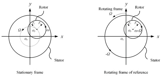
Figure 7.
Schematic diagram of steady method.
As the radial and tangential forces of the circular orbit model can be calculated with the steady method, the fluid-induced forces of the initial elliptical orbit model can be obtained with the steady method. The time-consuming transient computations can be avoided.
3.3. Rotordynamic Coefficient Identification
For each whirl frequency, the cases of Ωt = 0 rad and Ωt = π/2 rad are selected to identify the frequency-dependent rotordynamic coefficients. Substituting Ωt = 0 rad into Equation (15), the fluid-induced forces are expressed as:
Substituting Ωt = π/2 rad into Equation (15), the fluid-induced forces are expressed as:
Substituting Equations (16) and (17) into Equation (6), the frequency-dependent rotordynamic coefficients can be identified.
4. Numerical Model for Validation
4.1. Seal Geometry and Operating Conditions
To validate the orbit decomposition method, the results of the present method are compared with those of the transient CFD method. Considering that the time of transient computation is very long, a short seal with five teeth is taken as the research object. Figure 8 shows the seal geometry. Five seal teeth are installed on the stator. The rotor is smooth. The detailed geometry parameters of the labyrinth seal and operating conditions used for calculations are listed in Table 1.
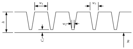
Figure 8.
Geometry of labyrinth seal.

Table 1.
Geometry parameters and operating conditions [14].
4.2. Computational Model and Mesh
Due to the circumferentially nonuniform flow pattern and fluid-induced forces acting on the rotor, a full 360 deg computational model and mesh are required. Figure 9 shows the computational model of the labyrinth seal. In order to ensure fully developed flow conditions, the upstream and downstream cavities are axially extended. The computational mesh is shown in Figure 10. More nodes are placed in the regions near the rotor and stator surfaces to catch the rotation and wall effects.
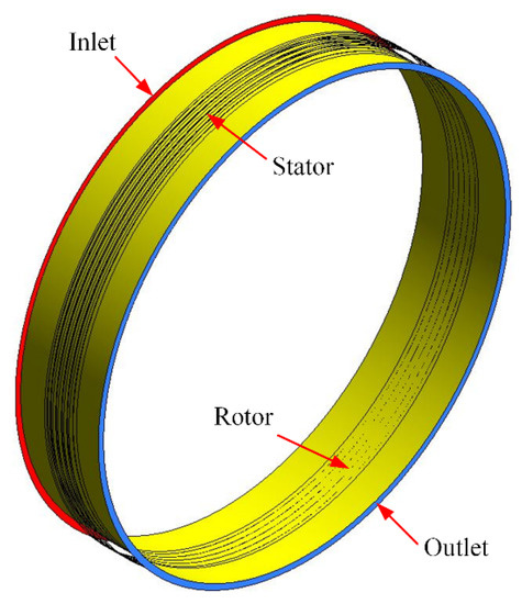
Figure 9.
Computational model of labyrinth seal.
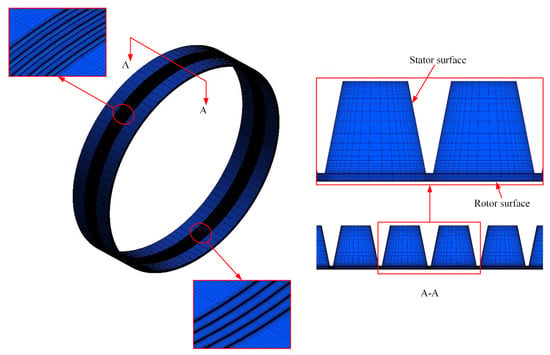
Figure 10.
Computational mesh of labyrinth seal.
In order to know how fine a mesh density is necessary for the accurate calculation, a mesh independence study is performed. The test is performed with a rotational speed of 1162 rad/s, inlet pressure of 3.447 MPa, outlet pressure of 1.724 MPa, and zero inlet preswirl. As shown in Figure 11, the test includes incremental adjustments to the grid size until the leakage and fluid-induced force results are independent. The final size of the mesh for the labyrinth seal is 7.69 × 10⁵ nodes.
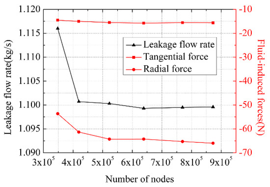
Figure 11.
Mesh independence study of leakage and fluid-induced forces.
4.3. Solution Technique
The CFD calculations are conducted with Ansys CFX software. The CFD analysis assumes the fluid to be ideal gas and the entire flow to be turbulent. The k-ε turbulence model is used because it can meet the requirements of excellent stability and accuracy [25,26,27]. The scalable wall function method is applied to describe the near wall flow conditions. These wall functions produce consistent results for grids of arbitrary refinement. The rotor and stator walls are defined to be adiabatic, smooth, and nonslip.
For the transient CFD method, the rotor surface, in addition to its rotational speed, is given a periodic elliptical orbit motion, specified by Equation (1). Five whirl frequencies ranging from 30 Hz to 150 Hz are considered in this study. For each frequency, 720 time steps are specified during each period. The transient computation is run for several whirl cycles until the periodicity of fluid-induced forces is reached. The steady solution is prepared for the initial condition of the transient computation. The steady solution is obtained in the case that the rotor and stator are concentric. The rotational speed, inlet total pressure, inlet temperature, and outlet static pressure are specified in the computation.
For the orbit decomposition method, two steady state simulations based on the circular orbit model are calculated. The amplitudes of the forward and backward circular orbit whirls are calculated according to Equation (8). Detailed calculating conditions for the two methods are listed in Table 2.
Table 2.
Calculating conditions.
5. Results and Discussion
5.1. Rotordynamic Results Comparison Between Two numerical Methods
The benefit of the orbit decomposition method is the ability to quickly calculate the transient fluid-induced forces and rotordynamic coefficients. In order to validate the present method, its rotordynamic results are compared with those of the traditional transient CFD method. According to a previous study [13], to capture the linear and small motion characteristics, the major semiaxis a is set to be 0.1 Cr, and the minor semiaxis b is set to be 0.5 a.
5.1.1. Fluid-Induced Forces
For the orbit decomposition method, the steady CFD method is used to calculate the tangential and radial forces of the two decomposed circular orbit models. The calculated tangential and radial forces are listed in Table 3. With the known tangential and radial forces, the time-dependent fluid-induced forces of the initial elliptical orbit model can be obtained according to Equation (15).
Table 3.
Tangential and radial forces of two decomposed circular orbit models.
For the transient CFD method, when the convergent solution of fluid-induced forces is obtained, the time-dependent fluid-induced forces during the last period are selected to compare with the orbit decomposition method. Taking the case of f = 30 Hz as an example, Figure 12 compares the time-dependent fluid-induced force results between the transient CFD method and the orbit decomposition method. Both methods capture the identical periodicity of the time-dependent fluid-induced forces. The fluid-induced forces can be expressed as a sinusoidal function:
where F is the fluid-induced force, A is the amplitude, and B is the initial phase.
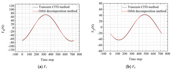
Figure 12.
Comparison of fluid-induced forces at f = 30 Hz.
For the two methods, the fluid-induced force amplitudes at different whirl frequencies are shown in Figure 13. The force amplitudes obtained with the two methods are very close. The maximum difference is less than 3.1%. With the increase in whirl frequency, the amplitudes of Fx and Fy increase. The initial phases of the fluid-induced forces are listed in Table 4. The initial phases of the orbit decomposition method are in good agreement with those of the transient CFD method. The maximum difference is less than 2%.
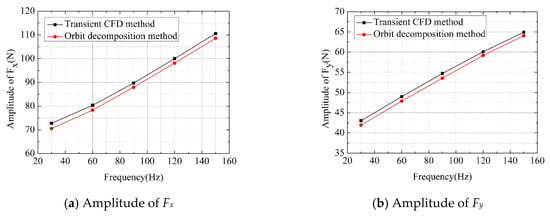
Figure 13.
Comparison of fluid-induced force amplitudes.
Table 4.
Initial phases of time-dependent fluid-induced forces at different whirl frequencies.
5.1.2. Rotordynamic Coefficients
When the time-dependent fluid-induced forces are obtained, the frequency-dependent rotordynamic coefficients can be determined according to Equation (6). Figure 14 shows the comparisons of rotordynamic coefficients determined with two methods. The two methods capture the identical frequency dependence of rotordynamic coefficients. The average differences of cross-coupled stiffness, direct stiffness, cross-coupled damping, and direct damping are 2.06%, 2.83%, 6.27%, and 2.67%, respectively. These two methods have the similar numerical accuracy.
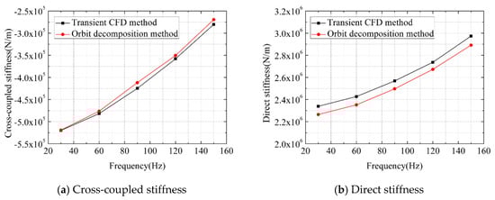
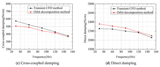
Figure 14.
Comparison of rotordynamic coefficients.
5.1.3. Computational Time
The CFD software is run on a computer with Intel Xeon E5−2650 v2 2.6 GHz CPU. Table 5 compares the computational times of two methods. For each frequency, the computational time for one transient calculation is about two days, while less than two hours is required for the orbit decomposition method. The computational time of the present method decreases by 96.44% relative to the transient CFD method.
Table 5.
Comparison of computational time for two methods.
5.2. Whirl Amplitude Analysis
For the orbit decomposition method, the influence of whirl amplitude is investigated by changing the major semiaxis a. Five values of major semiaxis a are studied, corresponding to 0.1 Cr, 0.2 Cr, 0.3 Cr, 0.4 Cr, and 0.5 Cr. For each major semiaxis a, the minor semiaxis b is set to be 50% of the major semiaxis a. The whirl frequency is 150 Hz.
Figure 15 shows the variations in rotordynamic coefficients with whirl amplitude. It can be found that the effect of whirl amplitude on the rotordynamic coefficients is very small and can be ignored when a < 0.2 Cr. This is because the rotor whirl is a small motion in this amplitude range. The rotordynamic system is linear, and the orbit decomposition method is valid to identify the rotordynamic coefficients. The rotordynamic coefficients are sensitive to the variation in whirl amplitude when a > 0.2 Cr. This is because the nonlinear effect becomes important in this amplitude range. The accuracy of the orbit decomposition method decreases with the increasing whirl amplitude. Similar findings can be obtained at other frequencies.
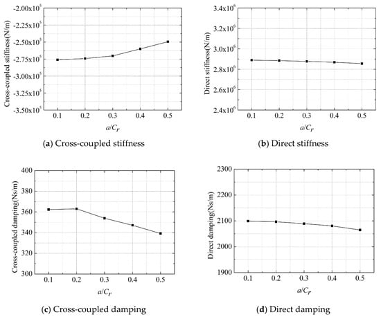
Figure 15.
Variations in rotordynamic coefficients with whirl amplitude.
5.3. Whirl Orbit Ellipticity Analysis
For the orbit decomposition method, the influence of orbit ellipticity is studied. The ellipticity λ is defined as:
The values for λ range from 0 to 1. Figure 16 shows the three typical whirl orbits. When major semiaxis a is equal to the minor semiaxis b, the value of λ is 0. The whirl orbit is a circle, as shown in Figure 16a. In this case, the present method cannot be used to identify the frequency-dependent rotordynamic coefficients according to Equation (6). When the minor semiaxis b is 0, the value of λ is 1. The whirl orbit is a straight line, as shown in Figure 16c. The present method is still effective to solve the frequency-dependent rotordynamic coefficients according to Equation (6).
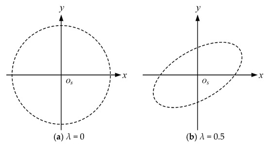
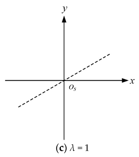
Figure 16.
Three typical whirl orbits.
In this analysis, the major semiaxis a is set to be 0.1 Cr, and three ellipticities are calculated by changing the minor semiaxis b, corresponding to a λ value of 0.1, 0.5, and 1. The whirl frequency is 150 Hz. Figure 17 shows the variations in rotordynamic coefficients with ellipticity λ. It can be found that the rotordynamic coefficients are not sensitive to the orbit ellipticity.
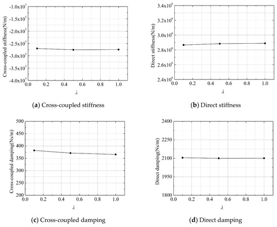
Figure 17.
Variations in rotordynamic coefficients with ellipticity.
6. Comparison with Experimental Data
To further validate the orbit decomposition method, its prediction results are compared with the experimental data tested on the high-pressure seal test rig owned by GE Oil & Gas [17]. The test object is the labyrinth seal. It has 14 teeth on the stator. The nominal diameter is 220 mm, radial clearance is 0.3 mm, tooth pitch is 5 mm, tooth height is 4 mm, tooth width at the tip is 0.2 mm, and tooth angle is 30 deg. At the seal upstream, the total pressure is 77.9 bar, static pressure is 72.3 bar, temperature is 12.5 °C, and preswirl ratio is 0.87. At the seal downstream, the static pressure is 50.6 bar. Five whirl frequencies are measured with a 10,000 rpm running speed. The detailed test conditions can be found in [17].
Figure 18 presents the rotordynamic coefficient comparisons between the present method and experimental data. Figure 18a–c show the whirl frequency effect on the cross-coupled stiffness, direct stiffness, and direct damping, respectively. The rotordynamic coefficients are predicted well. The prediction results capture the correct frequency dependence of rotordynamic coefficients. The cross-coupled stiffness and direct damping increase with the whirl frequency. The direct stiffness decreases with the whirl frequency. The cross-coupled stiffness and direct damping are two key parameters that affect the rotor stability. The positive cross-coupled stiffness tends to destabilize the rotor by adding energy to the forward whirl motion of the rotor. The positive direct damping tends to stabilize the rotor because it acts to remove energy from the forward whirl motion of the rotor. Considering these two coefficients comprehensively, the effective damping is defined as:
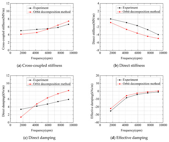
Figure 18.
Comparison of rotordynamic coefficients with the measured data.
Figure 18d depicts the effective damping versus whirl frequency. The predicted and measured results are in good agreement. The effective damping increases with the whirl frequency.
In general, the present method has good accuracy to predict the frequency-dependent rotordynamic coefficients for annular seals.
7. Limitations and Future Research Directions
The proposed method is valid when the whirl amplitude is less than 20% of seal clearance. When the whirl amplitude is larger than 20% of seal clearance, the accuracy of the proposed method decreases. The whirl amplitude should be carefully decided.
Additionally, only the widely used labyrinth seal is used as the research object in this article. In practice, many kinds of annular seals are applied, including the hole-pattern seal, honeycomb seal, and pocket damper seal. To further demonstrate the reliability and accuracy, the orbit decomposition method could be used to calculate the rotordynamic coefficients of all kinds of annular seals. The prediction results could be compared with the experimental data.
8. Conclusions
In this article, the orbit decomposition method based on small perturbation and linear superposition theory is proposed for the rapid identification of frequency-dependent rotordynamic coefficients for annular seals. Through the analysis and comparisons with the transient CFD method, several conclusions are summarized as follows:
- (1)
- Compared with the transient CFD method, the orbit decomposition method with steady state simulation can significantly reduce the computational time.
- (2)
- The orbit decomposition method and the transient CFD method have a similar accuracy in predicting the fluid-induced forces and rotordynamic coefficients.
- (3)
- The orbit decomposition method is valid when the whirl amplitude is less than 20% of the seal clearance. The accuracy of the orbit decomposition method decreases when the whirl amplitude is larger than 20% of the seal clearance.
- (4)
- The rotordynamic coefficients arising from the orbit decomposition method are not sensitive to the ellipticity.
Finally, the accuracy of the present method is further demonstrated with the experimental data. The present method provides a novel approach for the fast and accurate identification of frequency-dependent rotordynamic coefficients for annular seals.
The next research step is to use the proposed method to predict the rotordynamic coefficients of more annular seals, such as the hole-pattern seal, honeycomb seal, and pocket damper seal.
Author Contributions
Conceptualization, M.Z. and J.Y.; methodology, M.Z.; software, M.Z. and Q.G.; validation, M.Z., W.Z. and Q.G.; formal analysis, J.Y.; investigation, M.Z.; resources, J.Y.; data curation, M.Z.; writing—original draft preparation, M.Z.; writing—review and editing, J.Y.; visualization, M.Z.; supervision, J.Y.; project administration, J.Y.; funding acquisition, J.Y. and W.Z. All authors have read and agreed to the published version of the manuscript.
Funding
This research was funded by the National Natural Science Foundation of China, grant numbers 52075096 and 51875361.
Institutional Review Board Statement
Not applicable.
Informed Consent Statement
Not applicable.
Data Availability Statement
Data sharing is not applicable to this article.
Acknowledgments
The authors would like to acknowledge the support of National Natural Science Foundation of China, grant numbers 52075096 and 51875361.
Conflicts of Interest
The authors declare no conflict of interest.
Nomenclature
| a | Major semiaxis (m) |
| A | Amplitude of fluid-induced forces (N) |
| b | Minor semiaxis (m) |
| B | Initial phase (rad) |
| c | Cross-coupled damping (Ns/m) |
| C | Direct damping (Ns/m) |
| Cr | Seal clearance (m) |
| f | Whirl frequency (Hz) |
| F | Fluid-induced force (N) |
| Fr | Radial force (N) |
| Ft | Tangential force (N) |
| Fx | x direction component of the fluid-induced force (N) |
| Fy | y direction component of the fluid-induced force (N) |
| h | Seal cavity height (m) |
| k | Cross-coupled stiffness (N/m) |
| K | Direct stiffness (N/m) |
| n | Number of seal teeth |
| Pi | Inlet pressure (MPa) |
| Po | Outlet pressure (MPa) |
| r | Whirl radius (m) |
| R | Rotor radius (m) |
| t | Time (s) |
| T | Temperature (K) |
| Vi | Preswirl velocity (m/s) |
| w1 | Seal cavity width (m) |
| w2 | Tooth tip thickness (m) |
| w3 | Tooth root thickness (m) |
| X | x direction rotor displacement (m) |
| Y | y direction rotor displacement (m) |
| α | Ellipse attitude angle (rad) |
| λ | Ellipticity |
| ω | Rotational speed (rad/s) |
| Ω | Rotor whirl velocity (rad/s) |
| ∆t | Time step (s) |
| Subscripts | |
| b | Backward circular orbit whirl model |
| f | Forward circular orbit whirl model |
| i | Inlet |
| o | Outlet |
| r | Radial direction |
| t | Tangential direction |
| x | x direction |
| y | y direction |
| Superscripts | |
| 0 | Ωt = 0 rad condition |
| 1 | Ωt = π/2 rad condition |
| Abbreviations | |
| CFD | Computational fluid dynamics |
References
- Liang, D.; Gui, X.M.; Jin, D.H. Influence of Seal Cavity Leakage Flow on Compressor Performance Investigated with a Circumferentially Averaged Method. Appl. Sci. 2021, 11, 780. [Google Scholar] [CrossRef]
- Du, Q.; Zhang, D. Numerical Investigation on Flow Characteristics and Aerodynamic Performance of a 1.5-Stage SCO2 Axial-Inflow Turbine with Labyrinth Seals. Appl. Sci. 2020, 10, 373. [Google Scholar] [CrossRef]
- Cao, L.H.; Wang, J.X.; Li, P.; Hu, P.F.; Li, Y. Numerical Analysis on Steam Exciting Force Caused by Rotor Eccentricity. Shock. Vib. 2017, 2017, 8602965. [Google Scholar] [CrossRef]
- Xu, Q.; Niu, J.K.; Yao, H.L.; Zhao, L.C.; Wen, B.C. Fluid-Induced Vibration Elimination of a Rotor/Seal System with the Dy-namic Vibration Absorber. Shock Vib. 2018, 2018, 1738941. [Google Scholar]
- Jeon, S.M.; Kwak, H.D.; Yoon, S.H.; Kim, J. Rotordynamic analysis of a high thrust liquid rocket engine fuel (Kerosene) turbopump. Aerosp. Sci. Technol. 2013, 26, 169–175. [Google Scholar] [CrossRef]
- Tsukuda, T.; Hirano, T.; Watson, C.; Morgan, N.R.; Weaver, B.K.; Wood, H.G. A Numerical Investigation of the Effect of Inlet Preswirl Ratio on Rotordynamic Characteristics of Labyrinth Seal. J. Eng. Gas Turbines Power 2018, 140, 082506. [Google Scholar] [CrossRef]
- Cangioli, F.; Chatterton, S.; Pennacchi, P.; Nettis, L.; Ciuchicchi, L. Thermo-elasto bulk-flow model for labyrinth seals in steam turbines. Tribol. Int. 2018, 119, 359–371. [Google Scholar] [CrossRef]
- Iwatsubo, T.; Motooka, N.; Kawai, R. Flow Induced Force of Labyrinth Seal. In Proceedings of the Workshop on Rotordynamic Instability Problems in High-Performance Turbomachinery, College Station, TX, USA, 18 December 1982; NASA Lewis Research Center: Cleveland, OH, USA, 1982; pp. 205–222. [Google Scholar]
- Wyssmann, H.R.; Pham, T.C.; Jenny, R.J. Prediction of Stiffness and Damping Coefficients for Centrifugal Compressor Laby-rinth Seals. J. Eng. Gas. Turbines Power 1984, 106, 920–926. [Google Scholar] [CrossRef]
- Nordmann, R.; Weiser, P. Evaluation of Rotordynamic Coefficients of Look-Through Labyrinths by Means of a Three Volume Bulk Flow Model. In Proceedings of the Workshop on Rotordynamic Instability Problems in High-Performance Turbomachinery, Houston, TX, USA, 1 October 1991; NASA Lewis Research Center: Cleveland, OH, USA, 1991; pp. 147–163. [Google Scholar]
- Dereli, Y. Comparison of rotordynamic coefficients for labyrinth seals using a two-control volume method. Proc. Inst. Mech. Eng. Part A J. Power Energy 2008, 222, 123–135. [Google Scholar] [CrossRef]
- Wu, T.C.; San Andrés, L. Gas Labyrinth Seals: On the Effect of Clearance and Operating Conditions on Wall Friction Factors—A CFD Investigation. Tribol. Int. 2019, 131, 363–376. [Google Scholar] [CrossRef]
- Moore, J.J. Three-Dimensional CFD Rotordynamic Analysis of Gas Labyrinth Seals. J. Vib. Acoust. 2003, 125, 427–433. [Google Scholar] [CrossRef]
- Hirano, T.; Guo, Z.L.; Kirk, R.G. Application of Computational Fluid Dynamics Analysis for Rotating Machinery-Part Ⅱ: Labyrinth Seal Analysis. J. Eng. Gas. Turbines Power 2005, 127, 820–826. [Google Scholar] [CrossRef]
- Nielsen, K.K.; Jønck, K.; Underbakke, H. Hole-Pattern and Honeycomb Seal Rotordynamic Forces: Validation of CFD-Based Prediction Techniques. J. Eng. Gas Turbines Power 2012, 134, 122505. [Google Scholar] [CrossRef]
- Ertas, B.H.; Delgado, E.A.; Vannini, G. Rotordynamic Force Coefficients for Three Types of Annular Gas Seals with Inlet Preswirl and High Differential Pressure Ratio. J. Eng. Gas Turbines Power 2012, 134, 042503. [Google Scholar] [CrossRef]
- Vannini, G.; Cioncolini, S.; Del Vescovo, G.; Rovini, M. Labyrinth Seal and Pocket Damper Seal High Pressure Rotordynamic Test Data. J. Eng. Gas Turbines Power 2013, 136, 022501. [Google Scholar] [CrossRef]
- Thorat, M.R.; Hardin, J.R. Rotordynamic Characteristics Prediction for Hole-Pattern Seals Using Computational Fluid Dynamics. J. Eng. Gas. Turbines Power 2020, 142, 021004. [Google Scholar] [CrossRef]
- Childs, D.W.; Arthur, S.; Mehta, N.J. The Impact of Hole Depth on the Rotordynamic and Leakage Characteristics of Hole-Pattern-Stator Gas Annular Seals. J. Eng. Gas Turbines Power 2014, 136, 042501. [Google Scholar] [CrossRef]
- Vannini, G.; Thorat, M.R.; Childs, D.W.; Libraschi, M. Impact of Frequency Dependence of Gas Labyrinth Seal Rotordynamic Coefficients on Centrifugal Compressor Stability. In Proceedings of the ASME Turbo Expo: Power for Land, Sea and Air, Glasgow, Scotland, UK, 14–18 June 2010; ASME: New York, NY, USA, 2010; pp. 1–10. [Google Scholar]
- Chochua, G.; Soulas, T.A. Numerical Modeling of Rotordynamic Coefficients for Deliberately Roughened Stator Gas Annular Seals. J. Tribol. 2007, 129, 424–429. [Google Scholar] [CrossRef]
- Yan, X.; Li, J.; Feng, Z. Investigations on the Rotordynamic Characteristics of a Hole-Pattern Seal Using Transient CFD and Periodic Circular Orbit Model. J. Vib. Acoust. 2011, 133, 041007. [Google Scholar] [CrossRef]
- Yan, X.; He, K.; Li, J.; Feng, Z.P. Rotordynamic Performance Prediction for Surface-Roughened Seal Using Transient Compu-tational Fluid Dynamics and Elliptical Orbit Model. Proc. Inst. Mech. Eng. Part A J. Power Energy 2012, 226, 975–988. [Google Scholar] [CrossRef]
- Yan, X.; He, K.; Li, J.; Feng, Z. Numerical Investigations on Rotordynamic Characteristic of Hole-Pattern Seals with Two Different Hole-Diameters. J. Turbomach. 2015, 137, 071011. [Google Scholar] [CrossRef]
- Li, Z.G.; Li, J.; Feng, Z.P. Numerical Investigations on the Leakage and Rotordynamic Characteristics of Pocket Damper Seals—Part Ⅱ: Effects of Partition Wall Type, Partition Wall Number, and Cavity Depth. J. Eng. Gas. Turbines Power 2015, 137, 032504. [Google Scholar] [CrossRef]
- Li, Z.; Li, J.; Feng, Z. Numerical Comparison of Rotordynamic Characteristics for a Fully Partitioned Pocket Damper Seal and a Labyrinth Seal with High Positive and Negative Inlet Preswirl. J. Eng. Gas Turbines Power 2015, 138, 042505. [Google Scholar] [CrossRef]
- Gao, R.; Kirk, G. CFD Study on Stepped and Drum Balance Labyrinth Seal. Tribol. Trans. 2013, 56, 663–671. [Google Scholar] [CrossRef]


Publisher’s Note: MDPI stays neutral with regard to jurisdictional claims in published maps and institutional affiliations. |
© 2021 by the authors. Licensee MDPI, Basel, Switzerland. This article is an open access article distributed under the terms and conditions of the Creative Commons Attribution (CC BY) license (https://creativecommons.org/licenses/by/4.0/).