POCS-Augmented CycleGAN for MR Image Reconstruction

Abstract

Recent years have seen increased research interest in replacing the computationally intensive Magnetic resonance (MR) image reconstruction process with deep neural networks. We claim in this paper that the traditional image reconstruction methods and deep learning (DL) are mutually complementary and can be combined to achieve better image reconstruction quality. To test this hypothesis, a hybrid DL image reconstruction method was proposed by combining a state-of-the-art deep learning network, namely a generative adversarial network with cycle loss (CycleGAN), with a traditional data reconstruction algorithm: Projection Onto Convex Set (POCS). The output of the first iteration’s training results of the CycleGAN was updated by POCS and used as the extra training data for the second training iteration of the CycleGAN. The method was validated using sub-sampled Magnetic resonance imaging data. Compared with other state-of-the-art, DL-based methods (e.g., U-Net, GAN, and RefineGAN) and a traditional method (compressed sensing), our method showed the best reconstruction results.

1. Introduction

Magnetic resonance imaging (MRI) has become a standard diagnosis tool in clinic service due to the non-invasiveness, multiple contrasts, and high temporal and spatial resolutions it can provide. However, the speed of MRI is still much slower compared with the other imaging modalities such as computed tomography (CT) because of the sequential encoding paradigm used for acquiring the frequency- or phase-encoded raw data in the so-called k-space (the Fourier transform domain) [1]. Without sacrificing the image resolution and without hardware upgrading, an essential way to shorten the data acquisition time is to acquire a subset of the fully sampled k-space determined by the Nyquist sampling theory. An imperative step is then to reconstruct the MR image from the incomplete k-space data, as it was from a fully sampled k-space dataset. Tremendous MR image reconstruction methods have been developed over the past decades. Among them, parallel imaging is a popular choice which relies on recovering the missing k-space information using the spatially localized sensitivity profiles of the elements within a phase array coil [2,3,4,5,6]. Compressed sensing (CS) is another widely used reconstruction method which does not depend on the sensitivity encoding as in parallel imaging but rather on suppressing the incoherent or sparse noise caused by random or pseudo-random k-space sampling [7]. Both types of reconstruction methods and other methods often use an iterative process to solve a nonlinear optimization problem, which is time-consuming and sensitive to parameter selections. Outside of the MR research field, the past several years have seen sensational success from a variety of model-free deep neural networks in image classification [8], computer vision, auditory processing, information generation, and medical imaging [9,10,11,12]. Motivated by such superb performance of deep learning (DL) [13], different groups have incorporated various DL networks into MRI reconstructions such as a deep convolutional autoencoder network [14], deep residual learning [15], deep ADMM-net [16], U-Net [17], and Cycle-GAN [18].

While those pioneering studies have shifted MRI reconstruction from a model-based scenario to a new end-to-end learning-based era, most of the machine learning-based methods are still difficult to understand. Trained by limited data, the reconstruction performance may not be generalizable. By contrast, the well-established traditional methods are often guided by physics. Their generalizability is high. Combining the traditional methods and deep learning may provide a better solution that can incorporating merits from both types of image reconstruction algorithms. To assess this possibility, we proposed a hybrid deep learning based image reconstruction method in this study. Our method contains two steps: the first one is a regular DL-based image reconstruction process, and the second is a renewed version of step one but with the output of the DL network trained in step one included as additional training data. This framework is similar to the well-known traditional data reconstruction algorithm: Projection Onto Convex Set (POCS) [19]. From the point of view of DL, our method can be considered as a new data augmentation strategy, and we therefore dubbed the method as a POCS-augmented DL. A related study was reported in [18], where the authors used two sequentially concatenated generative adversarial networks (GANs) [20] to reconstruct the final MR images. Because of the sequential concatenation, the second GAN only sees residual artifacts in the output of the first one. By contrast, the POCS-augmented network sees both the original image artifacts due to the missing data points in the k-space and the residual artifacts due to the imperfect reconstruction of the first round of DL reconstruction, allowing the network to learn the artifact distribution at different noise levels and remove them from the reconstructed images. Another improvement is that we used Cycle-Consistent Adversarial Networks (CycleGAN) [21] as the reconstruction network, which has shown improved performance compared with a GAN.

The rest of the paper is organized as follows. In Section 2, we formulated the problem and introduce the proposed POCS-CycleGAN. In Section 3, we described the data-processing, implementation of the proposed POCS-CycleGan model, and training of the model. We evaluated the proposed model with several datasets and compare the proposed model with several state-of-the-art deep learning models in Section 4. We discussed our findings in Section 5. Finally, we concluded this paper in Section 6. A preliminary version of POCS-CycleGAN has been previously presented at a conference in 2018 [22].

2. Materials and Methods

2.1. Problem Definition and Notations

Denote $y\in C^N$ ($C$ is the complex domain, and $N$ is the dimension) as the desired image to be restored, which consists of $\sqrt{\mathrm{N}}\times \sqrt{\mathrm{N}}$ pixels, where the undersampled k-space data is represented by $x\in C^M$, in which M << N. Denote the linear operator (undersampling process) with ${ℱ}_{𝓊}\in C^{M\times N}$, which can be further represented by ${ℱ}_{𝓊}=ℛℱ$. The image reconstruction problem under the condition of sub-Nyquist sampling is to recover the image $y$ from ${ℱ}_{𝓊}y$. For 2D image reconstruction, $ℱ\in C^{N\times N}$ is the two-dimensional discrete Fourier transform, and $ℛ\in C^{M\times N}$ is an undersampling mask used to select signals in the k-space to be sampled. The same concept can be extended to 3D image reconstruction by extending the 2D operators into 3D ones. For a nonlinear undersampling operator, the corresponding image reconstruction process is often formulated to be an optimization problem:

$$\underset{y}{min}\mathcal{S}\left(x\right)+\mathsf{\lambda }|x-{ℱ}_{𝓊}y.{|}_{l_2}^2$$

(1)

where $\mathcal{S}$ is a regularization term on $x$, $\mathsf{\lambda }$ is the data fidelity of the noise level of the acquired measurements $x$ [23], and $l_2$ is the Euclidean norm.

By using the deep learning reconstruction method, the problem can be defined by Equation (2):

$$\underset{y}{min}|y-f_{DL}\left(y_u|\theta \right){|}_{l_2}^2+\mathsf{\lambda }|x-{ℱ}_{𝓊}y{|}_{l_2}^2$$

(2)

where $f_{DL}$ is the forward mapping of the deep learning network with parameters $\theta$, $\mathsf{\lambda }$ allows the adjustment of the data fidelity, $y_u$ represents zero-filled reconstruction from under the sampled k-space where $y_u={ℱ}_{𝓊}^{\mathscr{H}}x$, and superscript $\mathscr{H}$ is the conjugated transpose operation.

The final reconstruction image is the output of the deep learning network and can be expressed as in Equation (3):

$$\widehat{y}=f_{DL}\left(y_u|\theta ,\mathsf{\lambda },\mathsf{\Omega }\right)$$

(3)

where $\mathsf{\Omega }$ represents the prior information we obtain from the k-space.

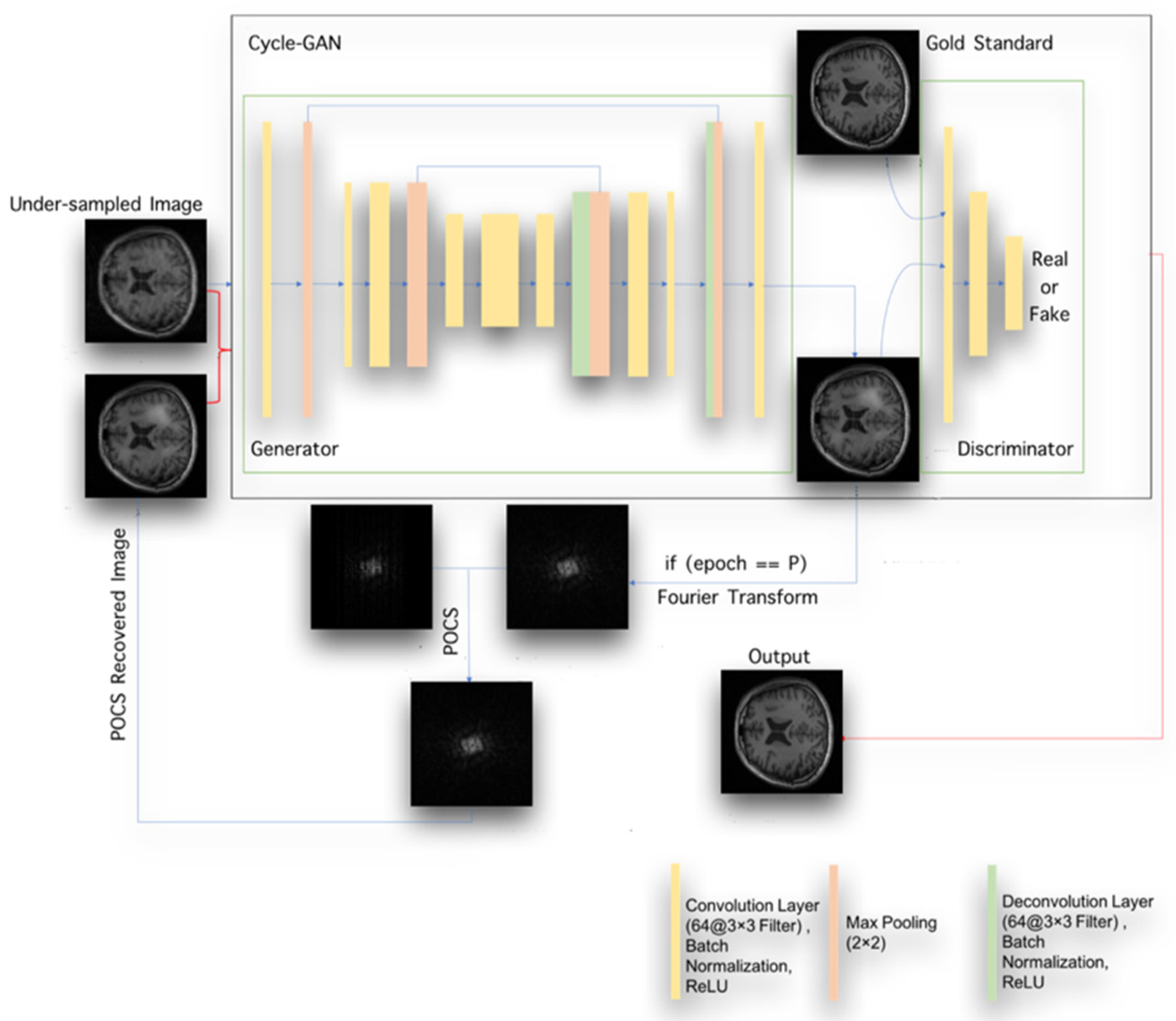
2.2. The Structure of the Entire POCS-Augmented CycleGAN (POCS-CycleGAN)

Figure 1 provides an overview of the proposed POCS-augmented CycleGAN. Two iterative CycleGANs [21] with the same network structures were involved, which differed by the training samples; the outputs of the first-pass CycleGAN after training were used as additional training samples for the second-pass CycleGAN.

The use of CycleGAN in image reconstruction is for building a generative model that learns mapping from undersampled images to fully sampled images. The performance of the generator is enhanced by using the discriminator to distinguish the real fully sampled data from the data created by the generator. Our goal is to train generator $G_{u2f}$ to generate high-quality reconstructed images from undersampled images. CycleGAN uses two mirrored training processes as shown in Figure 2 to achieve this goal. Each training process involves training two generators and one discriminator.

Figure 2 shows the first part of the training process, which is to train generator $G_{u2f}$ and $G_{f2u}$ and discriminator $D_y$. The discriminator $D_y$ was trained first by fully sampled image $y$ so that it could learn the data distribution of the real fully sampled images. Then, generators $G_{u2f}$ and $G_{f2u}$ were trained in order. Generator $G_{u2f}$ projected the undersampled image $y_u$ (directly reconstructed from the undersampled k-space data x after filling the unacquired k-space locations by 0 s) into a recovered fully sampled one $\widehat{y}$. The output of $G_{u2f}$, $\widehat{y}$ was fed into discriminator $D_y$ and generator $G_{f2u}$ simultaneously. Discriminator $D_y$ needed to make decision of whether the input came from the real fully sampled dataset or from the reconstructed fully sampled images. The output of discriminator $D_y$ would be used as a part of the neuron network’s loss function (see Section 2.4.3. Adversarial Loss). Generator $G_{f2u}$ needed to generate $\widehat{y}$ back to the undersampled image, ${\widehat{y}}_u$. We wanted ${\widehat{y}}_u$ to look as similar to $y_u$ as possible so that the generated reconstructed image $\widehat{y}$ had high accuracy. We calculated the similarity by measuring the value of $|{\widehat{y}}_u,y_u{|}_{l_1}^1$, where $l_1$ means the L1 distance between ${\widehat{y}}_u$ and $y_u$. The smaller the value of $|{\widehat{y}}_u,y_u{|}_{l_1}^1$ was, the more similar ${\widehat{y}}_u$ and $y_u$ looked, which means the reconstructed image from $G_{u2f}$ had higher accuracy. The value of $|{\widehat{y}}_u,y_u{|}_{l_1}^1$ would also be used as a part of the neuron network’s loss function (explained in Section 2.4.3). Therefore, during this training process, $G_{u2f}$ was adjusted to generate reconstructed image $\widehat{y}$ to look as similar to the fully sampled ground truth image $y$, while $D_y$ was adjusted to maximally avoid being fooled by the intermediately reconstructed image.

The opposite direction’s training was similar to the aforementioned method. The function of this training process is to assist the first training process to train the generator $G_{u2f}$ as accurately as possible. After training the entire CycleGAN for several epochs (P), the output of $G_{u2f}$, $\widehat{y}$ was inversely transformed back to the k-space and updated by POCS. The POCS-processed output images of the first-pass CycleGAN of all training samples were added to the original training dataset to be used as the new and augmented training data for the second-pass CycleGAN. The whole training process is illustrated in Algorithm 1.

Algorithm 1 POCS-CycleGAN training.
Input:
$y_u$:	image from under-sampled k-space dataset
$y$:	image from fully-sampled k-space dataset
$\widehat{y_u}$:	under-sampled image generated from model
$\widehat{y}$:	fully-sampled image generated from model
P:	total epoch number
M:	epoch number to perform POCS
$K$:	k-space image
mask:	undersample mask
$ℱ$:	Fourier transformation
q:	POCS sample selection number
Output:
	for epoch = 0 to P do
	tem=0 /* a temporary variable to store the data processed by POCS */
	$\widehat{y_u}$←$G_{f2u}\left(y\right)$
	$\widehat{y}$←$G_{u2f}\left(y_u\right)$
	if epoch % M == 0 then
	$K_{y_u}$$=\mathrm{fft}\left(y_u\right)$
	$K_{POC{S}_y}$$=(\mathrm{mask}==0)?K_{y_u}$,$K_y$
	$POC{S}_y$$=ifft\left(K_{POC{S}_y}\right)$
	${\mathrm{SSIM}}_{\mathrm{POCS}}$ $=\mathrm{SSIM}(POC{S}_y$$,ifft\left(K_{POC{S}_y}\right))$
	$\mathrm{tem}+=(POC{S}_y,{\mathrm{SSIM}}_{\mathrm{POCS}})$
	end
	$\mathrm{Randomly}\mathrm{select}\mathrm{q}\mathrm{from}\mathrm{tem},\mathrm{yielding}\widehat{y_q}$
	$\widehat{y}$ ←$\widehat{y}{{\displaystyle \cup }}^{}\widehat{y_q}$
	$\mathrm{train}{G}_{u2f}$$,G_{f2u}$$,D_y$,$D_{y_u}$
	end

2.3. Architectures of the Generator and Discriminator

The generator was composed of U-Net, which consisted of two mirrored components: the contraction part and the expansion part. The contraction part included 6 convolution layers. Each layer had a different number of filters (see Figure 3). The filter size was 3 3. A stride of 1 in both directions with zero padding was used. After each convolution layer, the rectified linear unit (ReLU) [24] and batch normalization [25] were applied. The second convolutional layer was followed by a residual block (not shown in Figure 1, with details about the residual block explained in Figure 3) and a max pooling layer that had a step size of 1 along both directions. In the expansion part, the contraction feature map was attached to the same-sized up-pooling feature map. Figure 3 shows the architecture of the generator.

For discriminator D, we adopted the PatchGAN discriminator’s structure [26]. In Isola’s work, they demonstrated that because L1 or L2 loss can cause a blurry effect on image generation problems [27], they designed a new GAN discriminator structure that only modeled high-frequency structures. PatchGAN’s discriminator tries to judge if each $w\times w$ patch in an image is fake or real, where w is the size of the patch [26]. In our work, $w\times w$ was 32 × 32. The reason we adopted PatchGAN’s discriminator was to alleviate the blurry effect caused by L1 loss, which was used as a loss function for our networks. The detail of the loss function will be discussed in the loss function section. The structure of our discriminator was a convolutional neural network. This CNN consisted of 3 convolutional layers, 1 residual block, and another convolutional layer. For each convolutional layer, the kernel size and step size were set as 33 and 11, respectively. After each convolutional layer, ReLU and batch normalization were applied. For the residual blocks used in both the generators and the discriminators, the number of output channels was the same as the number of input channels. It includes two convolutional layers with a kernel size 3 × 3 and step size 1. The output of the first convolution layer would pass through batch normalization, the active function (ReLU), and the second convolution layer with the same parameters. We then obtained the final output of the basic residual block. The residual block used in the generator and in the discriminator were the concatenation of 4 and 5 basic residual blocks, respectively.

2.4. Loss Function

The goal of an image reconstruction GAN is to train the generator $G_{u2f}$ to transform the zero-filled reconstruction $y_u$ to a fully reconstructed image $\widehat{y}$. Meanwhile, the discriminator $D_y$ is trained to judge whether the image generated by $G_{u2f}$ is the same as the gold standard (i.e., the image from the fully sampled k-space data). At each training epoch, $G$ and $D$ were sequentially adjusted so that the images generated by $G$ could maximally approximate the references. $D$ was subsequently adjusted to tell the difference between the generated images and the references. We explained each loss function separately in the following subsections.

2.4.1. Discriminator’s Loss

For the discriminator $D_y$, we trained it with real fully sampled image y at first. After training, $D_y$ learned the data distribution of $y$, and $D_y$’s output was a $w\times w$ matrix, as we mentioned in the “Discriminator Architecture” subsection before. We called this matrix $w_y$. The ideal value of each element in this matrix was 1.

Then, the reconstructed image $\widehat{y}$ from generator $G_{u2f}$ was fed into the trained $D_y$. The output of $D_y$ was matrix $w_{\widehat{y}}$ of a size $w\times w$ as well. The ideal value of each element in $w_{\widehat{y}}$ was 0, but the real value of each value in $w_{\widehat{y}}$ and $w_y$ was a number between 0 and 1. The closer the value of each element in $w_{\widehat{y}}$ to 1, the more similar the generated image $\widehat{y}$ looked to the real image y. A similar strategy was also used in the discriminator $D_{y_u}$.

The goal of discriminators is to minimize the value of the following equation:

$${\left(w_y-1\right)}^2+w_{\widehat{y}}^2$$

(4)

where 1 is a matrix that has the same size as $w_y$, and each of its elements are 1. This equation means the discriminator $D_y$ can separate the real image and the generated image from the generator $G_{u2f}$ accurately.

2.4.2. Generator’s Loss

The goal of generator $G_{u2f}$ is to generate an image $\widehat{y}$ that looks as similar to the real image y as possible. This means generator $G_{u2f}$ needs to minimize the value of

$${\left(w_{\widehat{y}}-1\right)}^2$$

(5)

This equation means the generated image from generator $G_{u2f}$ looks so similar to the real image that the discriminator $D_y$ cannot separate the real image and the generated image accurately.

2.4.3. Adversarial Loss

We applied Equations (4) and (5) in our network to train the discriminator and generator separately, and the goal was to minimize the adversarial loss ${ℒ}_{\mathcal{G}\mathcal{A}\mathcal{N}}\left(G_{f2u},D_{y_u},y,x\right)$, which was defined by two parts.

For generator, it was defined by

$$E_{x\sim p_{data(x)}}\left[{\left(D\left(G\left(y_u\right)\right)-1\right)}^2\right]$$

(6)

where $G\left(y_u\right)$ means the generator takes an input $y_u$ converted by an inverse Fourier transform from the undersampled k-space data $x$, and $p_{data(x)}$ is the probability distribution of $x$.

For the discriminator, it was defined by

$$E_{y\sim p_{data(y)}}\left[{\left(D\left(y\right)-1\right)}^2\right]+E_{x\sim p_{data(x)}}\left[{\left(D\left(G\left(y_u\right)\right)\right)}^2\right]$$

(7)

where $D\left(y\right)$ means the discriminator takes the fully sampled image as an input, $D\left(G\left(y_u\right)\right)$ means the discriminator takes the reconstructed image from the generator as an input, and $p_{data(y)}$ is the probability distribution of $y$.

2.4.4. Cycle Loss

While the above loss function pushes the generator to transform an image with aliasing artifacts $y_u$[m] into an aliasing-free output $y$[ˆn], the output of the generator may not carry the same content as the input. This is because the discriminator was not trained with paired data (aliased image $y_u$[m] as the input and the corresponding aliasing-free image $y$[m] as the reference). To make sure the input and the output of the generator were images with the same contents, a cycle loss ${ℒ}_{𝒸𝓎𝒸}$ was used. ${ℒ}_{𝒸𝓎𝒸}$ calculated the difference between the output of $G_{u2f}\left(G_{f2u}\left(y\right)\right)$ and $y$ as well as $G_{f2u}\left(G_{u2f}\left(y_u\right)\right)$ and $y_u$. ${ℒ}_{𝒸𝓎𝒸}$ was defined by the following equation:

$${ℒ}_{𝒸𝓎𝒸}\left(G_{u2f},G_{f2u}\right)=E_{y\sim p_{data(y)}}|G_{u2f}\left(G_{f2u}\left(y\right)\right),y{|}_{l_1}^1+E_{x\sim p_{data(x)}}|G_{f2u}\left(G_{u2f}\left(y_u\right)\right),y_u{|}_{l_1}^1$$

(8)

The overall loss function was given by a weighted sum of the above sub-loss functions:

$$ℒ\left(G_{u2f},G_{f2u},D_{y_u},D_y\right)={ℒ}_{\mathcal{G}\mathcal{A}\mathcal{N}}\left(G_{u2f},D_y,x,y\right)+{ℒ}_{\mathcal{G}\mathcal{A}\mathcal{N}}\left(G_{f2u},D_{y_u},y,x\right)+\mathsf{\beta }{ℒ}_{𝒸𝓎𝒸}\left(G_{u2f},G_{f2u}\right)$$

(9)

where $\mathsf{\beta }$ is a regularization parameter to balance the weights of generative loss and cycle loss.

2.5. POCS

POCS [19] is a well-known method for solving optimization problems. It has been used in MR image reconstructions since a long time ago [28]. For supervised MR reconstruction from undersampled data, two convex sets could be defined: ${\mathsf{\varphi }}_1$ was the reference image set, and ${\mathsf{\varphi }}_2$ was the collection of images whose inverse Fourier transformed data matched the acquired data at the sampling k-space locations [29]:

$${\mathsf{\varphi }}_1=\{\widehat{y}\mid dist\left(\widehat{y},y\right)<\mathsf{\xi }\}$$

(10)

$${\mathsf{\varphi }}_2=\left\{\widehat{y}\mid ℱ\left\{\widehat{y}\right\}=x\left[i,j\right],\left[i,j\right]\in \mathsf{\Theta }\right\}$$

(11)

where $dist(,)$ means distance, $|\widehat{y},y{|}_{l_2}^2$. $\xi$ is a small constant defining the reconstruction accuracy, and $\mathsf{\Theta }$ indicates the sampled k-space locations. Projecting into the two convex sets could be implemented by a Fourier transform and inverse Fourier transform.

In our work, POCS served as a transition layer of the CycleGAN to generate a second dataset with a different statistical distribution from the original dataset. The details of implementing this idea were the following. After half of the training epochs, the output of the generator $G_{u2f}$, $y$, was first processed by soft thresholding $T$ to boost the reconstruction performance. Then, we applied an FFT to the boosted reconstruction image and processed it with POCS, where the k-space data of the intermediate reconstructed image would be replaced with the acquired k-space data at the sampled k-space positions as described in Equation (12) below.

The boosting process could be defined as $\widehat{y}=T\left(\widehat{y},\epsilon \right)$, in which $\epsilon$ is a random small number close to 0:

$$\left(\widehat{y}\left[i, j\right],\epsilon \right)=\{\begin{array}{c}0,if\left|\widehat{y}\left[i,j\right]\right|\le \epsilon \\ \frac{\left(\Vert \widehat{y}\left[i, j\right]\Vert -\epsilon \right)}{\Vert \widehat{y}\left[i, j\right]\Vert }\widehat{y}\left[i, j\right], otherwise\end{array}$$

(12)

$$X_{POCS}\left[i,j\right]=\{\begin{array}{c}{X}_{\mathrm{recon}}\left[i,j\right],ifx\left[i,j\right]=0\\ x\left[i,j\right],otherwise\end{array}$$

(13)

where $X_{\mathrm{recon}}\left[i,j\right]$ means the Fourier Transform of the reconstructed image $\widehat{y}$ and $X_{POCS}\left[i,j\right]$ means the value of the k-space data at the coordinate $\left[i,j\right]$. Equation (13) means that the generator G_u2f only generates the missing data from the original undersampled k-space. The new dataset is a mix of the original training dataset with the new generated dataset $X_{POCS}$ from the POCS layer as described in Equation (12). The new dataset is the concatenation of $y_{POCS}$ and $y_u$:

$$y_{POCS}={ℱ}^{\mathscr{H}}{X}_{POCS}$$

(14)

3. Experiments

This subsection includes the process of data preparation and the network training.

3.1. Datasets

POCS-CycleGAN was evaluated with two different datasets. Dataset 1 contained T1-weighted brain images from our local database. MR imaging was conducted in a 3-T whole body scanner (Siemens Medical Systems, Erlangen, Germany) using a 3D MPRAGE sequence with the following parameters: TR/TE/TI = 1620/3/950 ms. It included 800 images from 80 health subjects. We used 600 of them for training and 200 of them for testing. Dataset 2 contained knee MRI images from the open MRI dataset [30] from Facebook and NYU. Fully sampled knee MRIs were obtained at 3 or 1.5 tesla magnets and included coronal proton density-weighted images with fat suppression. The training dataset included 2240 undersampled images. The test dataset included 560 undersampled images.

3.2. Data Prepration

The size of all the images was 256 × 256. Undersampled images were generated from the fully sampled images in the k-space by multiplying the k-space data with an undesampling mask. Figure 4 shows some examples of the radial and Cartesian sampling trajectories associated with a sampling rate of 10% and 20% relative to the full sampling trajectory determined by the Nyquist sampling theory. The undersampled image $y_u$ was generated by $y_u={ℱ}_{𝓊}^{\mathscr{H}}ℛF\left(y\right)$, where $ℛ$ is the sampling operator defined by the binary sampling trajectory mask, and ${ℱ}_{𝓊}^{\mathscr{H}}$ represents the inverse Fourier transform here. For the brain dataset, the k-space data were generated from the real-valued, T1-weighted images using a Fourier transform, and a Cartesian undersampling mask was employed. For the knee images, the k-space data were obtained from the open MRI database, and a radial undersampling mask was adopted.

3.3. Network Training Procedures

We trained the discriminator and generator recursively, with discriminator training first followed by generator training. All network weights were randomly initialized. The loss function was minimized using the Adam optimizer, with a learning rate of 0.0002, beta 1 of 0.5, and a mini-batch size of 4 at each epoch. The number of epochs was 500. During training, the POCS was performed every 50 epochs.

3.4. Compared Methods

We compared the proposed POCS-CycleGAN to several state-of-the-art MR reconstruction methods:

• U-Net: U-Net is a seminal work originally proposed for end-to-end biomedical image segmentation [31]. In [17], the authors applied U-Net to the MR reconstruction task. We implemented and trained U-Net as suggested in the work of Hyun et al. (2018).
• GAN: The vanilla GAN [32] was used.
• CycleGAN: The network is the GAN with cycle loss, and the training process can be performed in the absence of paired examples [21].
• RefineGAN: RefineGAN is inspired by the CycleGAN [18] and is composed of a deeper generator network to boost the interpolation of the undersampled k-space data for accurate MR image reconstruction. The hyper-parameters were set the same as in [18].

3.5. Evaluation

The performance of the reconstruction was measured by two quantitative metrics: the Structure Similarity Index (SSIM), a perceptual metric that quantifies image quality degradation [33], and the Peak Signal-to-Noise Ratio (PNSR). A higher SSIM and PSNR indicates better image reconstruction quality. We also provided reader studies based on the radiologic score to further assess the reconstruction quality. The image quality was qualitatively assessed by two radiologists. Twenty samples as test subjects were randomly selected from the brain and knee datasets separately. Five different reconstruction methods were conducted to generate fully sampled images. The results were provided to the two radiologists independently without disclosing which method was used to process the image. The quality score ranged from 1 to 5, and the values meant (1) zero, (2) server noise, (3) moderate noise that disturbs evaluation, (4) mild noise that does not affect evaluation, and (5) clear reconstruction. A higher value indicated better recovery performance.

4. Results

Model training took about a day, but image reconstruction only took about 5 s for one image. The SSIM and PSNR evaluations of the brain and knee test sets are demonstrated in Figure 5. The quantitative PSNR and SSIM of the first dataset are shown in

Table 1. PSNR (mean standard deviation) of different methods with different sampling rates for the NYU dataset.

Sampling Rate	10%	20%
U-Net	19.67 ± 1.89	25.11 ± 1.86
GAN	20.51 ± 1.67	26.05 ± 1.75
CycleGAN	21.55 ± 1.79	26.05 ± 1.82
RefineGAN	22.83 ± 1.54	26.79 ± 1.84
POCS-CycleGAN	24.58 ± 2.59	27.86 ± 1.92

and

Table 2. SSIM (mean standard deviation) of different methods with different sampling rates for the NYU dataset.

Sampling Rate	10%	20%
U-Net	0.33 ± 0.09	0.39 ± 0.10
GAN	0.34 ± 0.09	0.46 ± 0.10
CycleGAN	0.38 ± 0.08	0.46 ± 0.07
RefineGAN	0.40 ± 0.08	0.52 ± 0.08
POCS-CycleGAN	0.42 ± 0.09	0.59 ± 0.10

, respectively. Figure 6 shows the reconstruction results for one representative undersampled dataset. The first row shows the reconstructed images under different methods. The second row shows the difference map between the reconstructed image and the fully sampled image. Across all voxels, POCS-CycleGAN produced the smallest reconstruction errors on average, as measured by the distance to the reference.

Figure 5a,c,e shows the PSNR performance of all the assessed reconstruction methods. When compared with compressed sensing (CS), all DL-based reconstruction methods except for the CycleGAN yielded higher PSNR values (p < 10⁻⁶, paired t-test). The POCS-CycleGAN produced a significantly higher PSNR than the CyleGAN. No significant PSNR difference was found between the POCS-CycleGAN and RefineGAN. The SSIM performances of all the methods are shown in Figure 5b,d,f. When compared with zero-filling and CS, all the DL-based methods, including U-Net, CycleGAN, RefineGAN and POCS-CycleGAN, produced higher SSIM values. All DL-based methods, including CycleGAN, produced higher SSIM values than CS. POCS-CycleGAN demonstrated the highest SSIM among these methods (p < 10⁻⁶, paired t-tests).

We show the PSNR and SSIM values of dataset 2 in Table 1 and Table 2, respectively.

The representative reconstruction results are shown in Figure 6, Figure 7 and Figure 8. We can observe that even at the lowest sampling rate, POCS-CycleGAN preserved the structure detail very well and showed good denoising performance in both the brain and knee datasets. The proposed method outperformed the traditional compressing method and other deep learning methods.

Figure 9 shows the radiologic score conducted separately by different methods over 20 subjects’ brain and knee MR images. U-Net, GAN, CycGAN, RefineGAN, and POCS-CycleGAN had average scores of 2.5, 2.6, 2.8, 2.95, and 3.3 from the first radiologist and 2.15, 2.35, 2.6, 2.35, and 2.7 from the second radiologist, respectively, in terms of knee MRIs. For the brain MRIs, the corresponding 5 methods had average scores of 2.7, 3.85, 3.4, 3.6, and 3.7 from the first radiologist and 2.2, 3.3, 3.2, 3.9, and 4.05 from the second radiologist, respectively. The results suggest that POCS-CycleGAN consistently achieved better results.

Figure 10 shows the training loss of POCS-CycleGAN trained on the brain dataset with the radial trajectory, and the sampling rate was 10%. The blue, yellow, green, and red curves indicate the loss for $D_{y_u},G_{u2f},D_y,G_{f2u}$, respectively. The loss curves bounce up and down with the iterations instead of decreasing consistently. The reason for this is POCS kept generating new datasets for training. Even though the losses did not drop, the model still learned the mapping relation from the undersampled data to the fully sampled data better since more data was included.

5. Discussion

We extended our previous work in integrating traditional MR image reconstruction with DL into a full paper to propose a hybrid MR image reconstruction algorithm. The new method is based on a combination of the CycleGAN and POCS. The former is a popular DL network that has been successfully applied to many research fields [34,35], and the latter is a standard optimization method that has been widely used in MR image reconstruction [36,37]. While the GAN was used in MR reconstruction in [18], we used the CycleGAN because of the additional data consistency constraint enforced in it. In fact, the two mirrored projection processes of CycleGAN highly resemble the back-and-forth projections in a POCS-based data reconstruction algorithm and can be treated as a learning-based POCS process. Therefore, the proposed POCS-CycleGAN then represents a natural combination of an implicit and an explicit POCS algorithm. The performance gain of POCS-CycleGAN against CycleGAN and others was mainly due to the increase in the sample size and the reduction of artifacts in half of the training samples. Doubling the training dataset during the training process is a way to balance the training difficulty of generators and discriminators. CycleGAN did not significantly outperform compressed sensing. One reason for this could be the increase in the network parameters due to the use of two networks and subsequently needing more training data than were used in this paper. All the other assessed DL methods outperformed compressed sensing, which is consistent with the DL-based MR work published before [18,38]. POCS-CycleGAN produced the highest SSIM, meaning a better recovery of the texture details of the images. While we only tested CycleGAN in this study, the same POCS-based augmentation process can be incorporated with other neural networks. Since POCS augmentation can be recursively applied several times, a POCS augmented network like POCS-CycleGAN may be highly valuable for applications with very limited training samples. Future work would be required to validate POCS-CycleGAN for high acceleration rates and for 3D reconstructions. Currently, POCS-CycleGAN directly learns the fully sampled images. Future work should be performed to test whether learning the artifact-dominated difference images such as those in [14] could further improve performance. Although we only tested the combination of DL and POCS, a similar idea can be tested for the combinations of DL and other traditional algorithms. For example, images reconstructed by the traditional methods can be directly treated as new training samples for successive DL-based reconstruction. Again, that would require future investigations.

We only evaluated POCS as a data augmentation approach but it can be incorporated into the final image reconstruction process. For example, we can add a new POCS layer in the end to replace the k-space data of the DL reconstructed images with the acquired k-space data at the sampled k-space positions.

POCS-CycleGAN was validated using MR data in a single coil. Extending it to multiple coils is straightforward by concatenating the data from all the coils during model training and image reconstruction. In other words, data from different coils will be treated as separate training samples and input. The output of the network for all coils can be easily combined to form the final image. We noted the variational network-based image reconstruction method [39] during our final manuscript preparation. Since our focus in this paper was to combine the traditional method and DL, a future work might be required to test whether this combination still works if the DL component is replaced by the variation networks.

In each experiment, the k-space undersampling trajectory is the same. While we did not assess the performance of the proposed method for different sampling trajectories or different acceleration factors, a direct extension of POCS-CycleGAN is retrain or refine the existing model with data sampled with different undersampling trajectories and acceleration rate.

6. Conclusions

We proposed an approach for MR image reconstruction by combining the DL (data-driven) model with a non-DL (knowledge-based) model. We have evaluated our proposed approach comprehensively and demonstrated quantitative improvement. The proposed POCS-CycleGAN can be easily adopted for other CNNs.

References

1. Twieg, D.B. The k-trajectory formulation of the NMR imaging process with applications in analysis and synthesis of imaging methods. Med. Phys. 1983, 10, 610–621. [Google Scholar] [CrossRef]
2. Griswold, M.A.; Jakob, P.M.; Heidemann, R.M.; Nittka, M.; Jellus, V.; Wang, J.; Kiefer, B.; Haase, A. Generalized autocalibrating partially parallel acquisitions (GRAPPA). Magn. Reson. Med. An Off. J. Int. Soc. Magn. Reson. Med. 2002, 47, 1202–1210. [Google Scholar] [CrossRef] [PubMed] [Green Version]
3. Pruessmann, K.P.; Weiger, M.; Scheidegger, M.B.; Boesiger, P. SENSE: Sensitivity encoding for fast MRI. Magn. Reson. Med. An Off. J. Int. Soc. Magn. Reson. Med. 1999, 42, 952–962. [Google Scholar] [CrossRef]
4. Sodickson, D.K.; Manning, W.J. Simultaneous acquisition of spatial harmonics (SMASH): Fast imaging with radiofrequency coil arrays. Magn. Reson. Med. 1997, 38, 591–603. [Google Scholar] [CrossRef] [PubMed]
5. Wang, Z.; Wang, J.; Detre, J.A. Improved data reconstruction method for GRAPPA. Magn. Reson. Med. An Off. J. Int. Soc. Magn. Reson. Med. 2005, 54, 738–742. [Google Scholar] [CrossRef]
6. Wang, Z.; Fernández-Seara, M.A. 2D partially parallel imaging with k-space surrounding neighbors-based data reconstruction. Magn. Reson. Med. An Off. J. Int. Soc. Magn. Reson. Med. 2006, 56, 1389–1396. [Google Scholar] [CrossRef]
7. Lustig, M.; Donoho, D.L.; Santos, J.M.; Pauly, J.M. Compressed sensing MRI. IEEE Signal Process. Mag. 2008, 25, 72–82. [Google Scholar] [CrossRef]
8. Krizhevsky, A.; Sutskever, I.; Hinton, G.E. Imagenet classification with deep convolutional neural networks. In Proceedings of the Advances in Neural Information Processing Systems, Lake Tahoe, NV, USA, 3–6 December 2012; pp. 1097–1105. [Google Scholar]
9. Xie, D.; Bai, L.; Wang, Z. Denoising Arterial Spin Labeling Cerebral Blood Flow Images Using Deep Learning. arXiv 2018, arXiv:1801.09672. [Google Scholar]
10. Li, Y.; Xie, D.; Cember, A.; Nanga, R.P.R.; Yang, H.; Kumar, D.; Hariharan, H.; Bai, L.; Detre, J.A.; Reddy, R.; et al. Accelerating GluCEST imaging using deep learning for B0 correction. Magn. Reson. Med. 2020, 84, 1724–1733. [Google Scholar] [CrossRef]
11. Zhang, L.; Xie, D.; Li, Y.; Camargo, A.; Song, D.; Lu, T.; Jeudy, J.; Dreizin, D.; Melhem, E.R.; Wang, Z.; et al. Improving Sensitivity of Arterial Spin Labeling Perfusion MRI in Alzheimer’s Disease Using Transfer Learning of Deep Learning-Based ASL Denoising. J. Magn. Reson. Imaging 2021. [Google Scholar] [CrossRef]
12. Dreizin, D.; Zhou, Y.; Fu, S.; Wang, Y.; Li, G.; Champ, K.; Siegel, E.; Wang, Z.; Chen, T.; Yuille, A.L. A multiscale deep learning method for quantitative visualization of traumatic hemoperitoneum at CT: Assessment of feasibility and comparison with subjective categorical estimation. Radiol. Artif. Intell. 2020, 2, e190220. [Google Scholar] [CrossRef] [PubMed]
13. LeCun, Y.; Bengio, Y.; Hinton, G. Deep learning. Nature 2015, 521, 436–444. [Google Scholar] [CrossRef]
14. Wang, S.; Su, Z.; Ying, L.; Peng, X.; Zhu, S.; Liang, F.; Feng, D.; Liang, D. Accelerating magnetic resonance imaging via deep learning. In Proceedings of the 2016 IEEE 13th International Symposium on Biomedical Imaging (ISBI), Prague, Czech Republic, 13–16 April 2016; pp. 514–517. [Google Scholar]
15. Lee, D.; Yoo, J.; Ye, J.C. Deep residual learning for compressed sensing MRI. In Proceedings of the 2017 IEEE 14th International Symposium on Biomedical Imaging (ISBI 2017), Melbourne, Australia, 18–21 April 2017; pp. 15–18. [Google Scholar]
16. Yang, Y.; Sun, J.; Li, H.; Xu, Z. Deep ADMM-Net for compressive sensing MRI. In Proceedings of the 30th Conference on Neural Information Processing Systems (NIPS 2016), Barcelona, Spain, 5–10 December 2016. [Google Scholar]
17. Hyun, C.M.; Kim, H.P.; Lee, S.M.; Lee, S.; Seo, J.K. Deep learning for undersampled MRI reconstruction. Phys. Med. Biol. 2018, 63, 135007. [Google Scholar] [CrossRef] [PubMed]
18. Quan, T.M.; Nguyen-Duc, T.; Jeong, W.-K. Compressed sensing MRI reconstruction using a generative adversarial network with a cyclic loss. IEEE Trans. Med. Imaging 2018, 37, 1488–1497. [Google Scholar] [CrossRef] [Green Version]
19. Haacke, E.M.; Lindskogj, E.D.; Lin, W. A fast, iterative, partial-Fourier technique capable of local phase recovery. J. Magn. Reson. 1991, 92, 126–145. [Google Scholar] [CrossRef]
20. Goodfellow, I.; Pouget-Abadie, J.; Mirza, M.; Xu, B.; Warde-Farley, D.; Ozair, S.; Courville, A.; Bengio, Y. Generative adversarial nets. In Proceedings of the Advances in Neural Information Processing Systems, Montreal, QC, Canada, 8–13 December 2014; pp. 2672–2680. [Google Scholar]
21. Zhu, J.-Y.; Park, T.; Isola, P.; Efros, A.A. Unpaired image-to-image translation using cycle-consistent adversarial networks. In Proceedings of the IEEE International Conference on Computer Vision, Venice, Italy, 22–29 October 2017; pp. 2223–2232. [Google Scholar]
22. Yang, H.; Wang, Z. POCS-augmented CycleGAN for MR image reconstruction. In Proceedings of the ISMRM Workshop on Machine Learning Part II, Washington, DC, USA, 25–28 October 2018. [Google Scholar]
23. Schlemper, J.; Caballero, J.; Hajnal, J.V.; Price, A.N.; Rueckert, D. A deep cascade of convolutional neural networks for dynamic MR image reconstruction. IEEE Trans. Med. Imaging 2017, 37, 491–503. [Google Scholar] [CrossRef] [Green Version]
24. Nair, V.; Hinton, G.E. Rectified linear units improve restricted boltzmann machines. In Proceedings of the ICML, Haifa, Israel, 21–24 June 2010. [Google Scholar]
25. Ioffe, S.; Szegedy, C. Batch normalization: Accelerating deep network training by reducing internal covariate shift. In Proceedings of the International Conference on Machine Learning, Lille, France, 6–11 July 2015; pp. 448–456. [Google Scholar]
26. Isola, P.; Zhu, J.-Y.; Zhou, T.; Efros, A.A. Image-to-image translation with conditional adversarial networks. In Proceedings of the IEEE Conference on Computer Vision and Pattern Recognition, Honolulu, HI, USA, 21–26 July 2017; pp. 1125–1134. [Google Scholar]
27. Larsen, A.B.L.; Sønderby, S.K.; Larochelle, H.; Winther, O. Autoencoding beyond pixels using a learned similarity metric. In Proceedings of the International Conference on Machine Learning, New York, NY, USA, 19–24 June 2016; pp. 1558–1566. [Google Scholar]
28. Haacke, E.M.; Liang, Z.-P.; Boada, F.E. Image reconstruction using projection onto convex sets, model constraints, and linear prediction theory for the removal of phase, motion, and Gibbs artifacts in magnetic resonance and ultrasound imaging. Opt. Eng. 1990, 29, 555–567. [Google Scholar] [CrossRef]
29. Chen, J.; Zhang, L.; Luo, J.; Zhu, Y. MRI reconstruction from 2D partial k-space using POCS algorithm. In Proceedings of the 2009 3rd International Conference on Bioinformatics and Biomedical Engineering, Beijing, China, 11–13 June 2009; pp. 1–4. [Google Scholar]
30. Zbontar, J.; Knoll, F.; Sriram, A.; Murrell, T.; Huang, Z.; Muckley, M.J.; Defazio, A.; Stern, R.; Johnson, P.; Bruno, M.; et al. fastMRI: An open dataset and benchmarks for accelerated MRI. arXiv 2018, arXiv:1811.08839. [Google Scholar]
31. Ronneberger, O.; Fischer, P.; Brox, T. U-net: Convolutional networks for biomedical image segmentation. In Proceedings of the International Conference on Medical Image Computing and Computer-Assisted Intervention, Munich, Germany, 5–9 October 2015; pp. 234–241. [Google Scholar]
32. Goodfellow, I.J.; Abadie, J.P.; Mirza, M.; Xu, B.; Farley, D.W.; Ozair, S.; Courville, A.; Bengio, Y. Generative adversarial nets. Adv. Neural Inf. Process. Syst. 2014, 27, 2672–2680. [Google Scholar]
33. Wang, Z.; Bovik, A.C.; Sheikh, H.R.; Simoncelli, E.P. Image quality assessment: From error visibility to structural similarity. IEEE Trans. Image Process. 2004, 13, 600–612. [Google Scholar] [CrossRef] [Green Version]
34. Godard, C.; Mac Aodha, O.; Brostow, G.J. Unsupervised monocular depth estimation with left-right consistency. In Proceedings of the IEEE Conference on Computer Vision and Pattern Recognition, Honolulu, HI, USA, 21–26 July 2017; pp. 270–279. [Google Scholar]
35. Hoffman, J.; Tzeng, E.; Park, T.; Zhu, J.-Y.; Isola, P.; Saenko, K.; Efros, A.; Darrell, T. Cycada: Cycle-consistent adversarial domain adaptation. In Proceedings of the International Conference on Machine Learning, Stockholm, Sweden, 10–15 July 2018; pp. 1989–1998. [Google Scholar]
36. Samsonov, A.A.; Kholmovski, E.G.; Parker, D.L.; Johnson, C.R. POCSENSE: POCS-based reconstruction for sensitivity encoded magnetic resonance imaging. Magn. Reson. Med. An Off. J. Int. Soc. Magn. Reson. Med. 2004, 52, 1397–1406. [Google Scholar] [CrossRef] [PubMed]
37. McGibney, G.; Smith, M.R.; Nichols, S.T.; Crawley, A. Quantitative evaluation of several partial Fourier reconstruction algorithms used in MRI. Magn. Reson. Med. 1993, 30, 51–59. [Google Scholar] [CrossRef] [PubMed]
38. Yang, G.; Yu, S.; Dong, H.; Slabaugh, G.; Dragotti, P.L.; Ye, X.; Liu, F.; Arridge, S.; Keegan, J.; Guo, Y.; et al. DAGAN: Deep de-aliasing generative adversarial networks for fast compressed sensing MRI reconstruction. IEEE Trans. Med. Imaging 2017, 37, 1310–1321. [Google Scholar] [CrossRef] [PubMed] [Green Version]
39. Hammernik, K.; Klatzer, T.; Kobler, E.; Recht, M.P.; Sodickson, D.K.; Pock, T.; Knoll, F. Learning a variational network for reconstruction of accelerated MRI data. Magn. Reson. Med. 2018, 79, 3055–3071. [Google Scholar] [CrossRef] [PubMed]
Figure 1. A schematic view of the POCS-augmented Cycle-GAN. The entire algorithm contains two recursive processes. Each has the same network structure but a different number of training samples. The output of the first process is used as new training samples in addition to the original training data after the following POCS reconstruction. The output of the first process is first inversely transformed into the Fourier domain. Then, the data of the sampled locations in the Fourier domain are replaced with the acquired ones, and the manipulated Fourier domain data are transformed back to the image domain. The generator is composed of a U-Net (Hyun et al., 2018) with skip connections. The discriminator uses a convolutional neural network. The functions of different layers are denoted by the legends at the bottom of the figure.
Applsci 12 00114 g001
Figure 2. The discriminator D y was trained first by fully sampled image y . Then, generator G u 2 f and G f 2 u were trained in order. The input of G u 2 f is the undersampled image, and the output of G u 2 f is reconstructed image y ^ . Then, y ^ was fed into discriminator D y and generator G f 2 u simultaneously. The discriminator was expected to distinguish y and y ^ . For G f 2 u , its output should be the reconstructed zero-filled images y ^ u . We forced y ^ u to be similar to y u by minimizing the value of y ^ u y u l 1 1 .
Applsci 12 00114 g002
Figure 3. The generator network structure. Yellow blocks represent convolutional layers with a kernel size 3 × 3, with ReLu as an activation function followed by batch normalization. Red blocks represent the max pooling layers. The black blocks represent residual blocks that includes two convolutional layers with kernel size 3 × 3. Green blocks represent the layer upsampled from the output of the previous residual block. The dimension of the layer represents the size and number of the input channels. The different calculation processes are represented by arrows with different colors, which are listed at the right foot of the figure. The size of the input image is 256 × 256, and the output size of the reconstructed image is 256 × 256.
Applsci 12 00114 g003
Figure 4. Radial and Cartesian sampling masks with different sampling rates (10% and 20%) in this study. White points indicate the sampled positions in the Fourier domain. The sampling rate is relative to the full sampling paradigm determined by the Nyquist sampling rule.
Applsci 12 00114 g004
Figure 5. SSIM and PSNR evaluations of the brain and knee test set.
Applsci 12 00114 g005
Figure 6. The fully sampled and undersampled brain images. The first and third rows are the brain images, and the second and fourth rows are the difference between the reconstructed image and the ground truth. The methods used for reconstructing the images are provided on top of each column. The undersampling rate was 20%, with a pseudo-random Cartesian sampling trajectory. The color bar is set between [0, 255].
Applsci 12 00114 g006
Figure 7. The fully sampled and undersampled knee images. The first and third rows are the knee images, and the second and fourth rows are the differences between the reconstructed image and the ground truth. The methods used for reconstructing the images are provided on top of each column. The undersampling rate was 10%, with a pseudo-random radial sampling trajectory. The color bar is set between [0, 255].
Applsci 12 00114 g007
Figure 8. The fully sampled and undersampled knee images. The first and third rows are the knee images, and the second and fourth rows are the differences between the reconstructed image and the ground truth. The methods used for reconstructing the images are provided on top of each column. The undersampling rate was 20%, with a pseudo-random radial sampling trajectory. The color bar is set between [0, 255].
Applsci 12 00114 g008
Figure 9. Comparison of radiologic scores between different methods over 20 subjects’ brain and knee MR images. Radiologic scores are displayed with five different colors. Vertical axis indicates the number of subjects for each radiologic score.
Applsci 12 00114 g009
Figure 10. The training loss of POCS-CycleGAN trained on the brain dataset with the radial trajectory, and the sampling rate was 10%. The four curves demonstrate the loss for D y u , G u 2 f , D y , G f 2 u .
Applsci 12 00114 g010