Abstract
This study presents the adoption of locally constrained regression models (LCRMs) with logarithmic transformations in order to model the flow stress behavior of the high-temperature deformation of 5005 aluminum alloy. Hot tensile tests for 5005 aluminum alloy were conducted under the temperatures of 290 °C, 360 °C, 430 °C, and 500 °C, and the strain rates of 0.0003/s, 0.003/s, and 0.03/s. The flow stress behavior was analyzed based on variations in temperature and strain rate. The flow stress during the hot deformation was modeled using the traditional Arrhenius type constitutive equation and the neural network approach. Then, for improved prediction accuracy, the flow stress was modeled using LCRMs. The prediction accuracies of the models were compared by calculating the MAE (Maximum Absolute Error) and RMSE (Root-Mean-Squared Errors) values. The MAE and RMSE of the LCRMs were lower than the errors of the Arrhenius equation and the neural network model. The results show that LCRMs can be useful in modeling the flow stress of 5005 aluminum alloy, and that the developed model can accurately predict the flow stress.
1. Introduction
5xxx series aluminum alloys—which contain magnesium (Mg) as the main alloying element—have good corrosion resistance, weldability, and strength to weight ratios [1,2,3], and they are also non-heat treatable. These advantages make such alloys premier materials for a wide range of applications, including vessel structures, ship construction, the automotive industry, the aircraft industry, the chemical industry, and food handling [2,3,4,5]. As a result, 5xxx aluminum alloys have attracted substantial research attention. For instance, the hot forming characteristics of the alloy have been examined in attempts to improve the production methods, reduce the cost, and improve the performance of aluminum products. To understand hot formability, it is essential to elucidate high-temperature deformation and flow stress behavior, and to derive the constitutive equation of the hot deformation. The constitutive equation explains the variation of stress as functions of various parameters, including strain rate, temperature, and strain. To date, many types of constitutive equations have been adopted to model the flow stress of the hot deformation of metallic alloys; the Arrhenius type constitutive equation based on the Zener-Hollomon theory has been the most widely used among them.
For instance, Tang et al. [6] studied the hot deformation of supersaturated Inconel 718 superalloy. In that study, the Inconel alloy was subjected to hot deformation tests at temperatures of 1100–1200 °C, and the flow stress was modeled using the Arrhenius type equation. Liu et al. [7] examined Hastelloy C-276 alloy through hot tensile tests at temperatures ranging between 1223–1423 K and strain rates ranging between 0.01–10/s. In that study, the flow stress was modeled using the modified Zerilli–Armstrong model, the modified Johnson-Cook model, and the modified Arrhenius model. The research findings showed that the modified type of the Arrhenius model predicted the flow stress best. Ohdar et al. [8] studied the high-temperature deformation of AISI 1035 steel. In that study, AISI 1035 steel was subjected to hot compression tests at temperatures ranging between 900–1100 °C and strain rates ranging between 0.2–20/s. They also accurately modeled the flow stress of AISI 1035 steel by adopting the Arrhenius constitutive equation. Thakur et al. [9] also used the Arrhenius equation to model the hot deformation flow stress of Nb-V-Ti micro-alloyed steel. In that study, hot compression tests were conducted on steel at temperatures ranging between 850–1100 °C and strains ranging between 1–100/s. The results showed that the Arrhenius type equation had a good level of performance. Traditionally, constitutive equations, including the Arrhenius equation, have been developed based on regression methods. However, regression-based constitutive equations often lack accuracy and efficiency in modeling complex flow stress behavior. Specifically, the relationships between flow stress and process parameters such as strain, strain rate, and temperature are highly nonlinear.
Therefore, a new modeling method using the neural network approach has been adopted [10,11,12,13,14,15]. For instance, Quan et al. [10] studied the hot deformation of 7050 Aluminum Alloy. In that work, hot compression tests for 7050 aluminum alloy were conducted at strain rates ranging between 0.01–10/s and temperatures ranging between 573 K and 723 K. The flow stress of 7050 aluminum alloy during the hot deformation was modeled using the improved type of Arrhenius equation and the neural network model. The performance of the neural network model was found to be better than that of the Arrhenius equation. Zhao et al. [11] performed hot compression tests of Ti600 titanium alloy at temperatures ranging between 760–920 °C and strain rates ranging between 0.01–10/s. The flow stress of the Ti600 titanium alloy was modeled using the Arrhenius equation, multiple linear model, and neural network model. The results showed that the predictions made by the neural network model were more accurate and efficient than those made by the other models.
Although the neural network approach has been successfully used to model hot deformation while substantially compensating for the drawbacks of the traditional constitutive equations, the neural network approach is limited by inefficiencies. As a result, there is still a crucial need to improve the modeling method, and this occurs in the development process. The development process involves the complex work of optimizing the process parameters, including the number of hidden layers, neurons, epochs, etc. The developed neural network model is sometimes computationally expensive. Furthermore, the neural network model is often inaccurate due to overfitting.
A literature review reveals the significance of new research adopting the new approach in modeling the flow stress of hot deformation. In other words, it is important to find a new highly efficient approach that makes accurate predictions. The research findings obtained using the new approach can be applied to research modeling the hot deformation of different types of metallic alloys.
The present work proposes a new modeling method for the high-temperature tensile deformation of 5005 aluminum alloy. First, the deformation characteristics were studied by discussing the flow stress behavior. The variation in flow stress was first modeled by the Arrhenius constitutive equation and the neural network model. Then, a newly proposed multiple modeling methodology consisting of locally constrained regression models (LCRMs) that use logarithmic transformations through switching was used; the logarithmic transformation of variables in a regression model is one of the most common ways to establish a nonlinear relationship between independent and dependent variables, and using the logarithm of one or more variables can effectively capture a nonlinear property while maintaining the linearity of the model [16]. Log transformation is also an effective method of transforming heavily skewed variables close to a normal distribution. Therefore, the predictive regression model for each domain was optimized through a logarithmic transformation to better express the nonlinearity of the flow stress.
The different models adopted in this research were compared to determine the comparative performance of locally constrained regression models (LCRMs) in terms of errors and reliability. This research aimed to contribute to the field of research searching for an efficient and accurate method for modeling the flow stress of hot deformation. Section 2 of this article explains the preparation of the test specimen and the process by which the hot tensile experiments were conducted. Section 3 describes the theory of the Arrhenius equation and LCRMs. In the Section 4, the measured stress and stress values predicted by the Arrhenius equation, neural network, and LCRMs are compared in terms of various aspects. Section 5 of this article provides the conclusion, which explains the limitations of the presented model and directions for future research.
2. Materials and Methods
2.1. Specimen Preparation
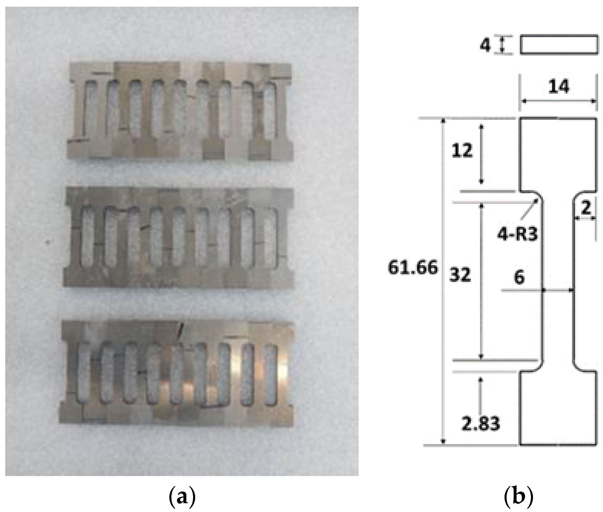
The 5005 aluminum tensile specimens were prepared in the rolling direction according to the ASTM-E8 standard. Planar specimens were used, and these were Wire EDM machined. The dimensions of the specimen were as follows: 4 mm thick, approximately 61.66 mm long, and 14 mm wide. Figure 1 shows the machined specimens and their dimensions. Table 1 lists the typical physical properties and material properties of 5005 aluminum alloy [17].
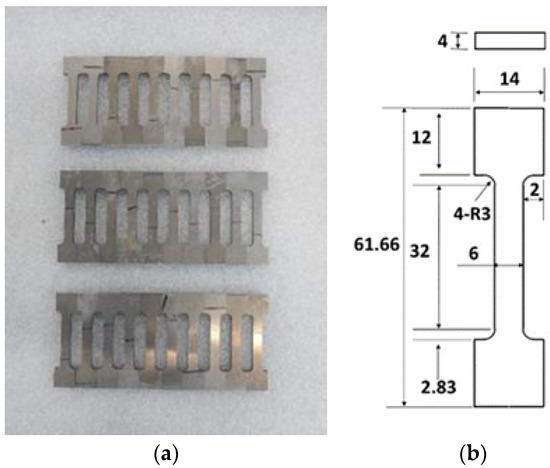
Figure 1.
(a) machined specimens and (b) dimensions (mm).

Table 1.
Physical and material properties of 5005 aluminum alloy.
2.2. Tensile Tests
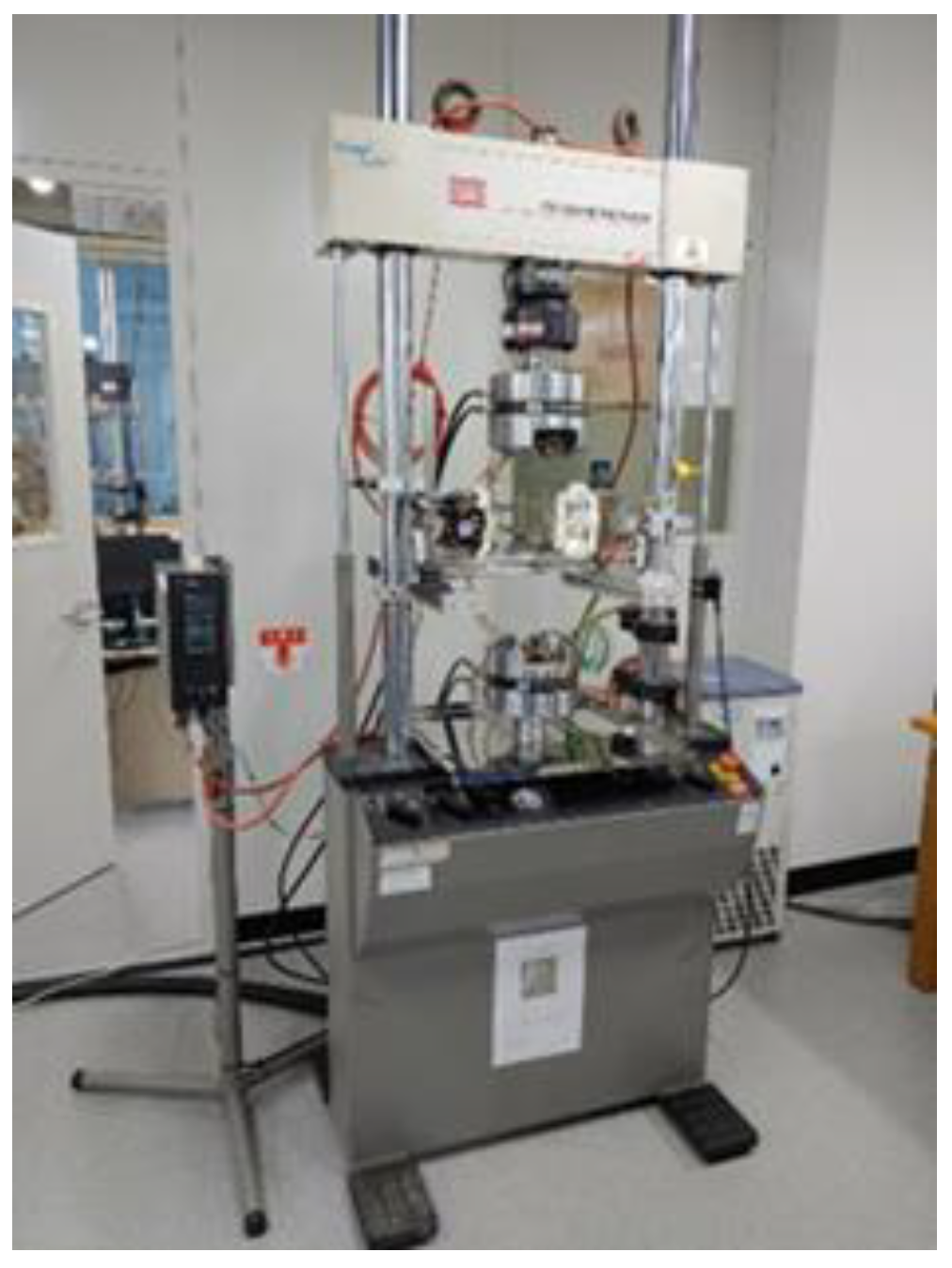
In this study, high-temperature tests were performed at temperatures of 290 °C, 360 °C, 430 °C, and 500 °C, as well as strain rates of 0.0003/s, 0.003/s, and 0.03/s at each temperature. The strain rates were considered to be similar than those in the hot rolling process. Figure 2 shows the test equipment (MTS-810 model) used for the tensile tests.
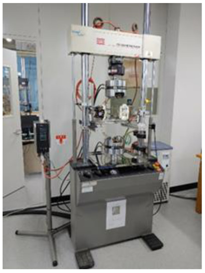
Figure 2.
Test equipment (MTS-810).
3. Flow Stress Modeling
3.1. Arrhenius Type Constitutive Equation
In the present work, the Arrhenius constitutive equation based on the Zener–Hollomon theory [18] was used to model the hot deformation flow stress of 5005 aluminum alloy. is the activation energy, while is the temperature and denotes the gas constant of . The Zener–Hollomon parameter was defined according to Equation (1).
In (1), denotes the strain rate defined in Equation (2) below,
where is the material constant and is the function, defined as (3):
In (3), σ is the stress and , , , and are the materials constants. After substituting the first, second, and third equations of (3) into Equation (2) and taking the logarithms of the three formulas, one can respectively obtain Equations (4)–(6):
After obtaining the equations, can be obtained by calculating the slope of plots, and can be obtained from the slope of the plots. The material constant is obtained by calculating the slope of the plots, and the constant can be obtained by calculating the slope of the plots.
After and are obtained, the material constant can be determined as in (7):
Equation (8) is obtained using (3) and (6) as below.
Then, the material constant A is calculated using the y-axis intercept of the plot. The obtained material constants , , , and are the functions of strain. In this research, the constants are described as 5th order polynomials, as indicated in (9)–(12). The coefficients of the polynomials obtained by regression are presented in Table 2.
Table 2.
Coefficient of polynomials.
The flow stress of the hot deformation can be derived using (2) and (3), as in (13).
In the present study, the flow stress was calculated through the Arrhenius equation using 25 selected points from each true stress–strain curve.
3.2. Locally Constrained Regression Model
A general way to model a nonlinear function, , is to approximate a model in the form , where is not linear with respect to the unknown parameters , or to transform the output variable, , and/or the input variable, , before estimating its linear regression model, . This translates into a nonlinear relationship between input and output, but the model itself is still linear in its parameters [19]. A commonly used input/output transformation is the (natural) logarithm, and the transformed model in log-log form can be expressed as [20]:
However, there are cases wherein simply transforming the data is not adequate for more complex representations of nonlinear characteristics, thus necessitating a more general specification. Assuming is simply a more flexible nonlinear function of , a better modeling approach would be to split the global nonlinear model into several parts and make them regionally linear, thus resulting in locally constrained regression models (LCRMs) such that [21,22]:
where is the number of local expert models and is the modeling error. As such, the concept of multiple modeling with switching is applied to allow the input feature domain to be naturally partitioned into multiple individual subtasks and to develop a relatively simple linear model for each partition in the region so that the set of developed models can be used to approximate the nonlinear properties [23]. As a result, multiple modeling schemes are very effective for modeling complex nonlinear systems. A smoother way to fit a nonlinear system is to use a piecewise quadratic or higher order trend rather than a piecewise line as described above. However, it is not recommended to fit a model higher than a quadratic to predict the stress of the aluminum alloy examined in this study because in the process of extrapolation, it can often be impractical to predict the outcome. Therefore, the least squares estimate of the parameters () is adopted due to its linearity in terms of the parameters.
From this point of view, the proposed modeling scheme consists of a set of regression models that approximate the stress properties of aluminum alloy, as well as a switching logic that selects the most optimized model based on its temperature. Figure 3 shows the overall architecture of the proposed multiple models with switching. The temperature value from 5005 aluminum alloy is provided as the input to the switching logic, which is translated into the regression model best suited to represent the stress with respect to properties such as strain and strain rate.
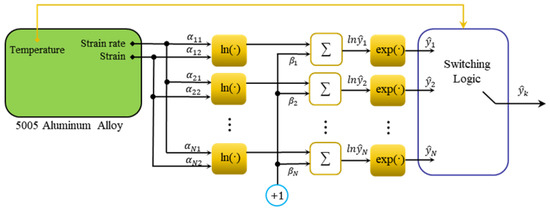
Figure 3.
Schematic of the proposed multiple models with switching used to predict the stress of 5005 aluminum alloy.
In summary, once each regression model is constructed via the least-squares method using the data sets of strain, strain rate, and flow stress included in each subdomain, the best fit regression model representing the flow stress is selected by the temperature-dependent switching logic of 5005 aluminum alloy.
4. Results and Discussion
4.1. Results
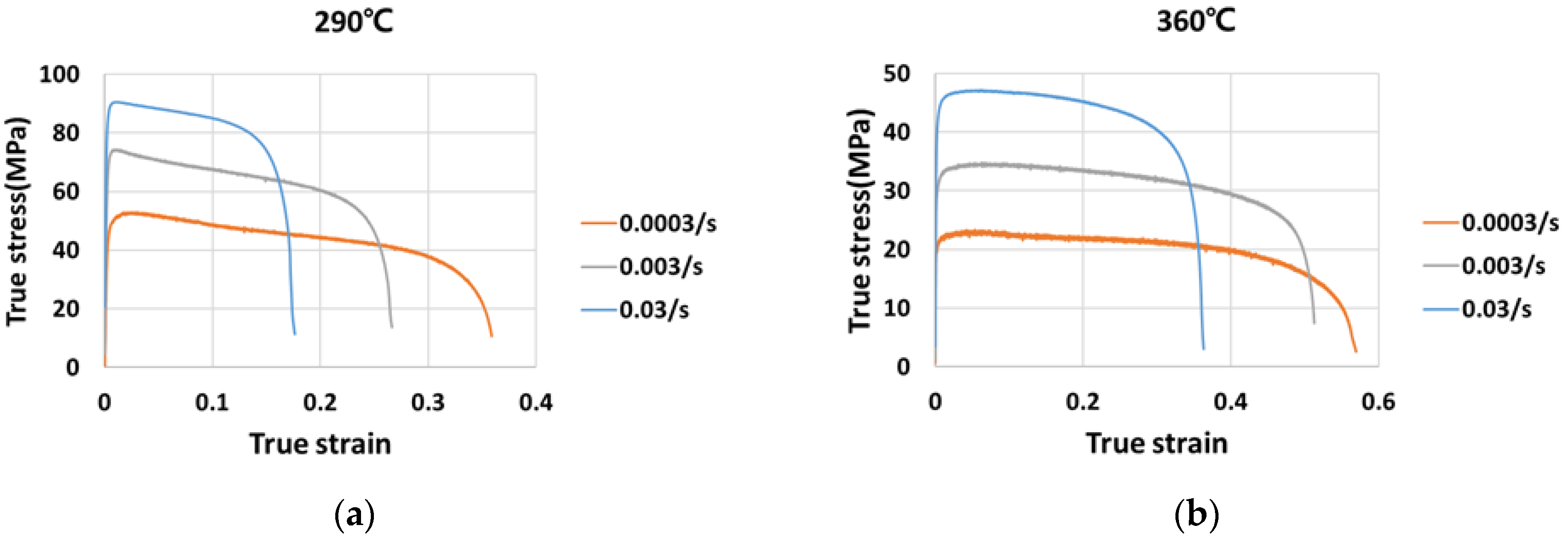
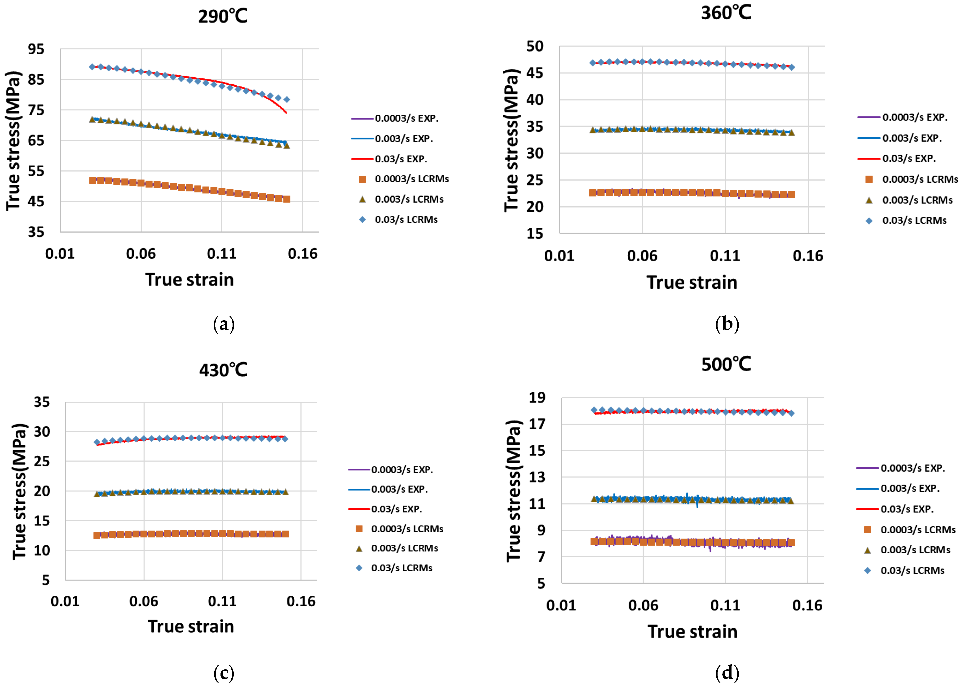
Figure 4 depicts true stress–strain curves at different temperatures. The variations in stress are considered to be largely dependent on variations in temperature and strain rate. The peak stress decreases with increases in temperature, while the peak stress increases with increases in strain rate. Maximum elongation was observed at 430 °C and 0.003/s, while minimum elongation was observed at 290 °C and 0.03/s.
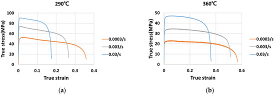
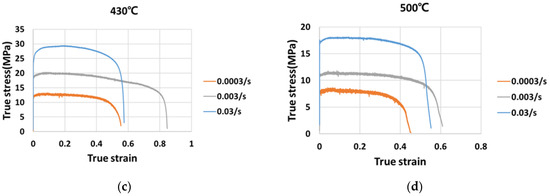
Figure 4.
True stress–strain curves at (a) 290 °C, (b) 360 °C, (c) 430 °C, and (d) 500 °C.
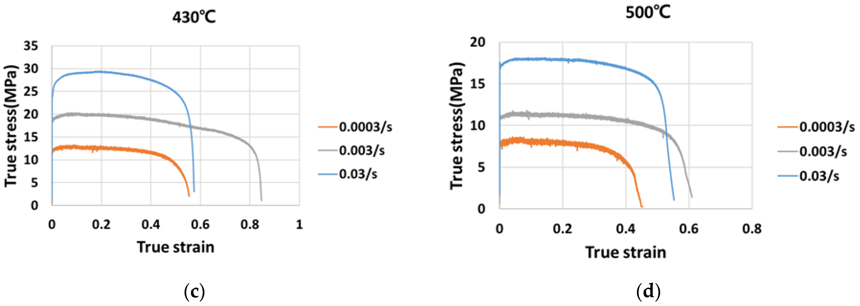
Figure 5 shows a comparison between the measured stress and the stress predicted by the Arrhenius equation at 290 °C, 360 °C, 430 °C, and 500 °C. The results show that the Arrhenius equation has low prediction accuracy. Specifically, it was observed that the prediction accuracy was significantly low at 290 °C. The MAE—defined as —of the predicted data was 4.515, while the RMSE—defined as —of the predicted data was 6.904.
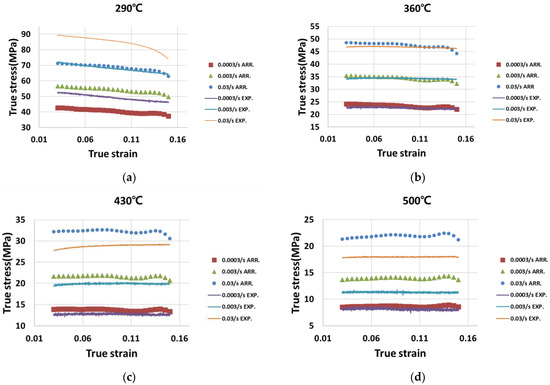
Figure 5.
True stress–strain curves by Arrhenius equation at (a) 290 °C, (b) 360 °C, (c) 430 °C, and (d) 500 °C.
To evaluate the predictive performance of the proposed LCRMs, data samples of strain, strain rate, and stress were extracted at temperatures of 290 °C, 360 °C, 430 °C, and 500 °C from 5005 aluminum alloy; therefore, four log-log regression models were created to predict the stress of aluminum alloy relative to the temperature. Each regression model had different properties to capture the overall stress dynamics, and the parameters were estimated by a vector consisting of the strain and strain rate of aluminum alloy obtained from 348 samples. After optimizing the parameters, a set of multiple models was tested with a series of 87 new data samples. For comparison with the proposed modeling scheme, a Neural Network (NN)—a representative nonlinear global model—was employed, and the selected number of neurons in the hidden layer of the NN was 20.
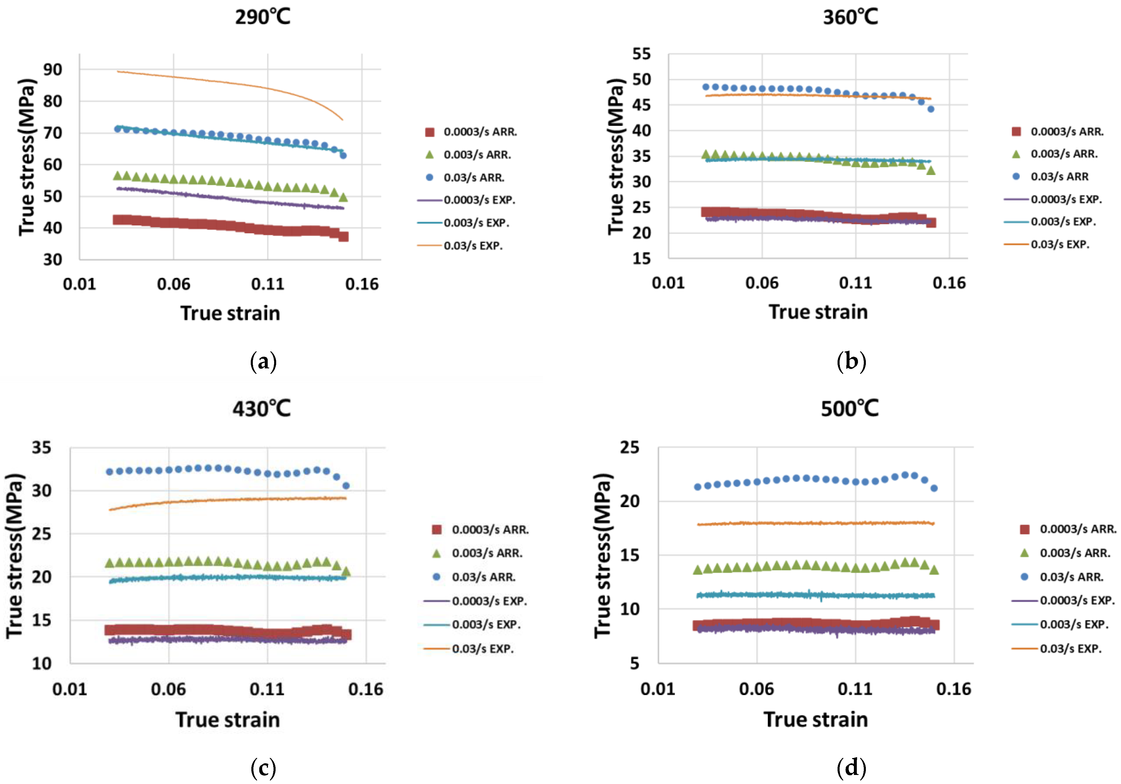
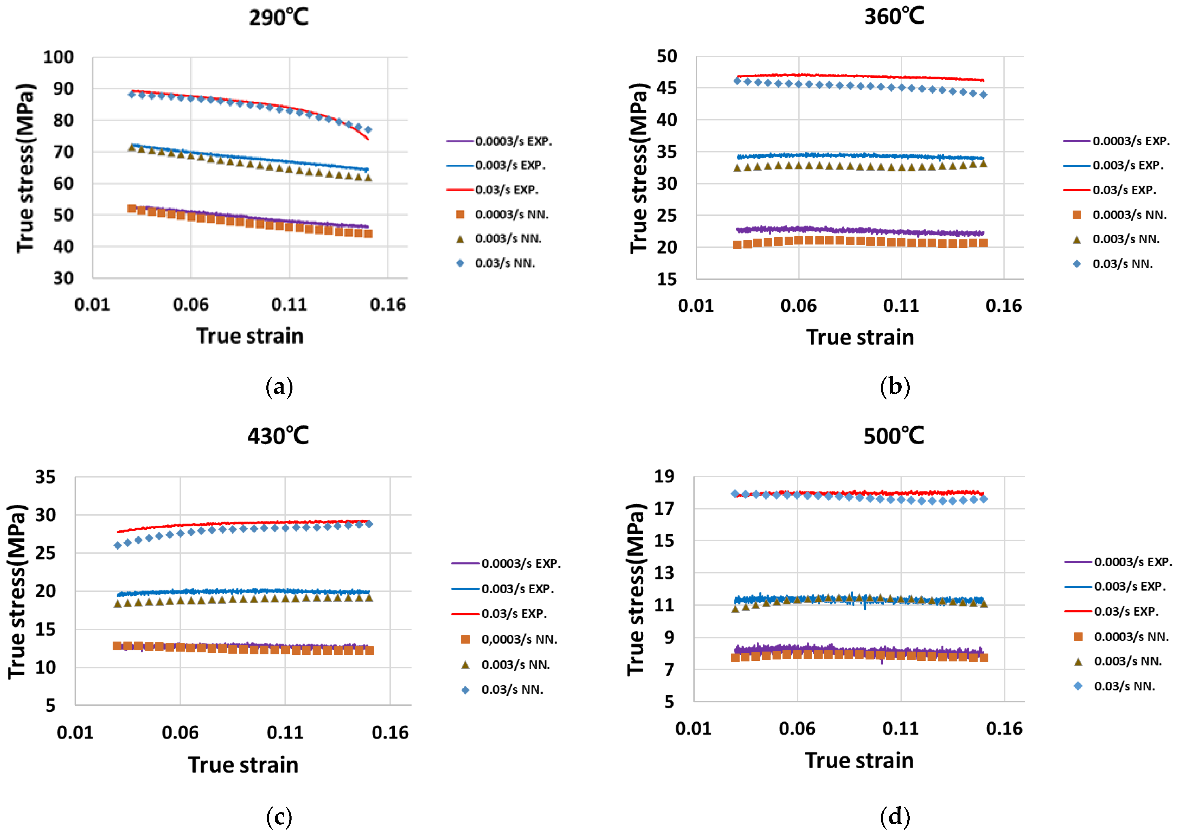
Figure 6 shows the comparison between the measured stress and the stress predicted by the Neural network at 290 °C, 360 °C, 430 °C, and 500 °C. The accuracy of the predictions made by the Neural network were substantially improved compared to those made by the Arrhenius equation. Furthermore, Figure 7 depicts the comparison between the measured stress and the stress predicted by LCRMs at 290 °C, 360 °C, 430 °C, and 500 °C. The prediction made by the LCRMs is shown to predict the flow stress with the best accuracy.
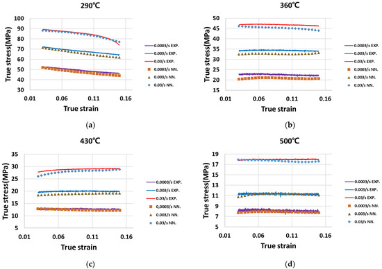
Figure 6.
True stress–strain curves by Neural Network at (a) 290 °C, (b) 360 °C, (c) 430 °C, and (d) 500 °C.
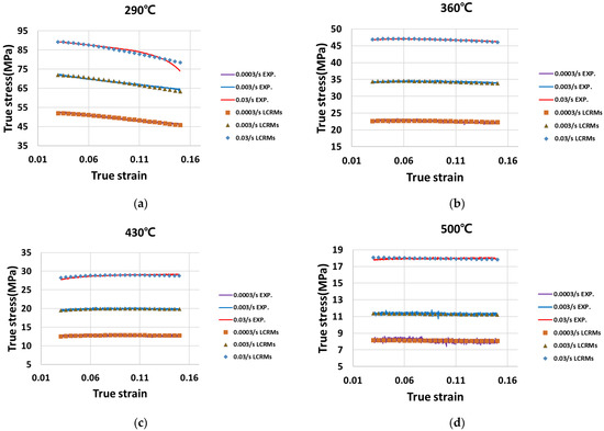
Figure 7.
True stress–strain curves by LCRMs at (a) 290 °C, (b) 360 °C, (c) 430 °C, and (d) 500 °C.
4.2. Discussion on the Performances of the Algorithms
Table 3 presents a comparison of the predictive performances of different models evaluated in terms of Maximum Absolute Error (MAE) and Root-Mean-Squared Errors (RMSE). The best result with LCRM was an RMSE of around 0.432, while the best result with a conventional global model, NN, was an RMSE of about 1.229. This result demonstrates that the proposed LCRMs scheme with switching is superior to a single global nonlinear model.
Table 3.
MAE and RMSE for three methods.
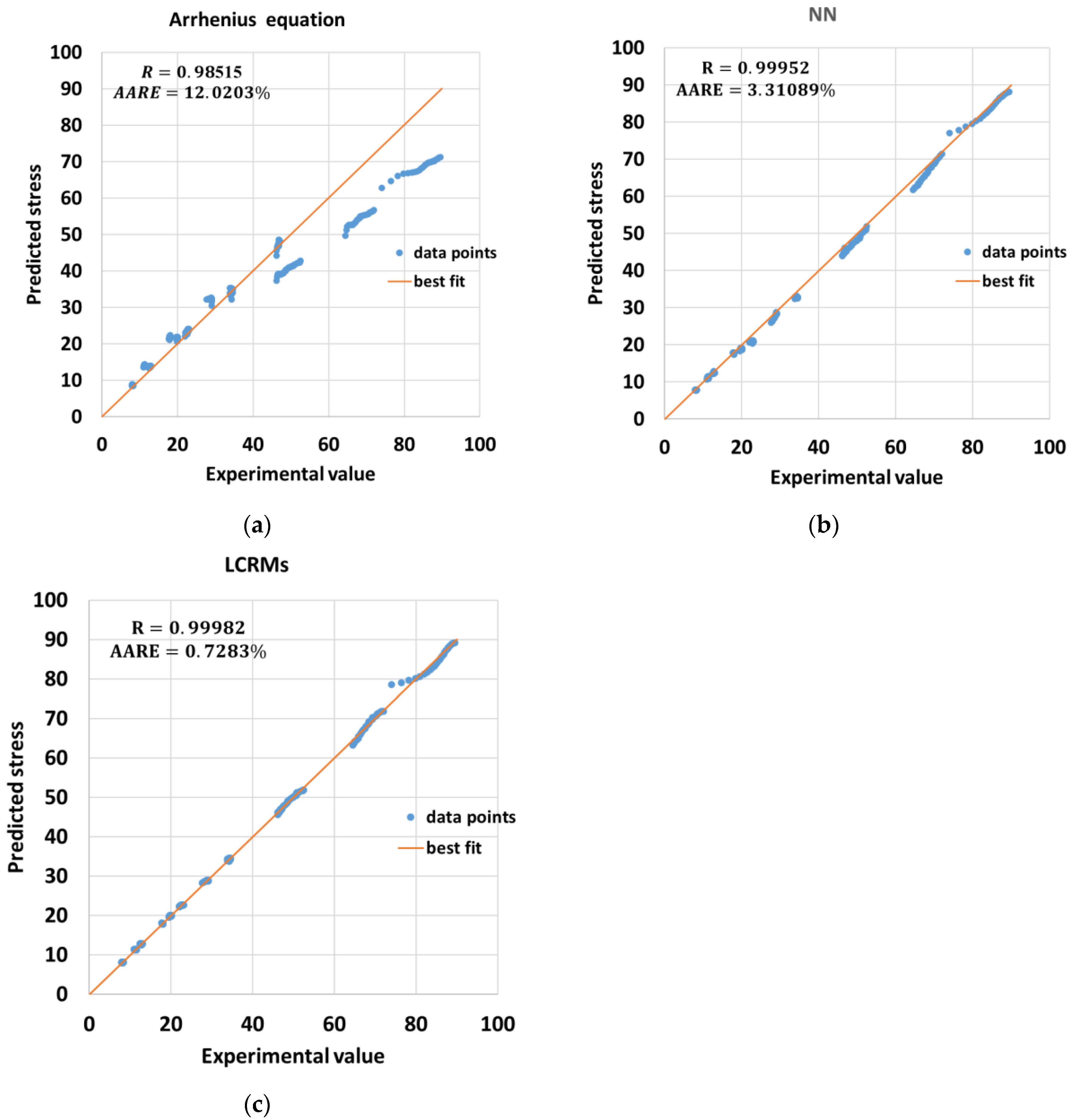
In this research, the accuracy of the different models was further evaluated by calculating the correlation coefficient denoted as as well as the Average Absolute Relative Error (AARE). Figure 8 shows the correlation between the experimental value and the predicted value by different models along with the and AARE values for each model. The and AARE values of the LCRMs are observed to be superior compared to those of the Arrhenius equation and NN. This indicates that the LCRMs have the most accurate performance.
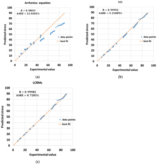
Figure 8.
Correlation between experimental value and predicted value by (a) Arrhenius equation, (b) NN, and (c) LCRMs.
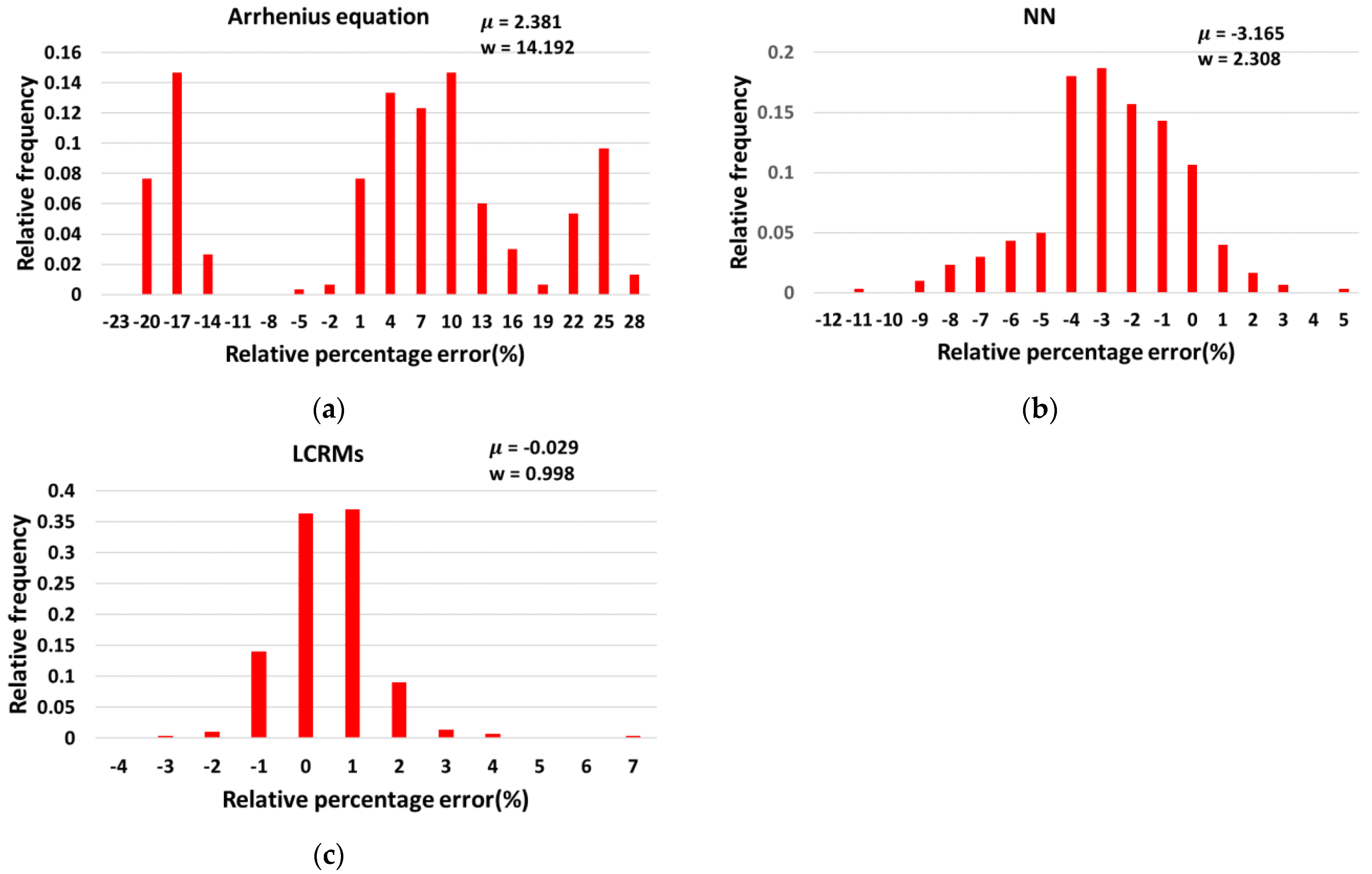
Studies were performed to obtain the relative percentage errors of the three different models. Figure 9 shows the relationships between relative percentage error and relative frequency for the (a) Arrhenius equation, (b) NN, and (c) LCRMs. In each plot, the relative percentage errors were indicated by the mean error value μ and the standard deviation w. The absolute value of the mean of the relative percentage error by LCRMs was 0.029 while the absolute values of the mean obtained by the Arrhenius equation and NN were 2.381 and 3.165, respectively. The standard deviation of the relative percentage error obtained by the LCRMs was 0.998 while the standard deviations of the error derived by the Arrhenius equation and NN were 14.192 and 2.308, respectively. The results showed that the errors by the Arrhenius equation and NN were dispersed. The study of the relative percentage error indicates that the performances of the LCRMs were the most reliable compared to the Arrhenius equation and the NN. Meanwhile, it should be noted that the absolute value of the mean of the relative percentage error obtained by the traditional Arrhenius equation is smaller than that obtained by the NN, while the standard deviation of the relative percentage error obtained by the Arrhenius equation is larger than the standard deviation obtained by the NN. The current research implies that the presented LCRMs are superior to the Arrhenius equation and NN in terms of prediction error and reliability. Further, the modeling using the LCRMs showed the best efficiency.
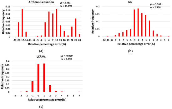
Figure 9.
Relative percentage error by (a) Arrhenius equation, (b) NN, and (c) LCRMs.
5. Conclusions, Limitations, and Future Research
5.1. Conclusions
In this research, the hot deformation flow stress of 5005 aluminum alloy was modeled using Locally Constrained Regression Models with Logarithmic Transformations (LCRMs), the Arrhenius equation, and a neural network (NN). The MAE and RMSE values obtained by the LCRMs were smaller than those obtained by the Arrhenius equation and the NN. The investigation of and AARE also indicated that the LCRMs are the most superior. The study of the relative percentage errors indicated that the performance of the LCRMs was the most reliable.
The MAE and RMSE values obtained by the LCRMs were 0.227 and 0.432, respectively, while the respective errors obtained by the Arrhenius equation were 4.515 and 6.904 and the respective errors obtained by the NN were 1.009 and 1.229. Therefore, the modeling by the LCRMs was found to be the most accurate.
The correlation coefficients R and AARE obtained by the LCRMs were about 0.98515% and 12.0203%, respectively, while the R and AARE values obtained by the Arrhenius equation were 0.99952% and 3.31089%, respectively, and the R and AARE values obtained by the NN were 0.99982% and 0.7283%, respectively.
The absolute value of the mean of the relative percentage error by LCRMs was 0.029 and the standard deviation of the relative percentage error by the LCRMs was 0.998. The absolute value and the standard deviation by the Arrhenius equation were 2.381 and 14.192, respectively, while the absolute values and the standard deviation by the NN were 3.165 and 2.308, respectively. Therefore, the results showed that the LCRMs were most reliable.
The absolute mean of the relative percentage error by the NN was larger than the absolute mean value of the Arrhenius equation, while the standard deviation by the NN was smaller than the standard deviation of the Arrhenius equation. The superiority of both the Arrhenius equation and NN needs to be investigated further.
5.2. Limitations and Future Research
In the current research, there were difficulties in extrapolation, and the LCRMs could not properly predict the stress for higher strain rates than those used in the given experimental data. This provided directions for future research.
Author Contributions
Conceptualization, J.C. and S.-H.S.; methodology, J.C. and S.-H.S.; software, J.C. and S.-H.S.; validation, J.C. and S.-H.S.; formal analysis, J.C. and S.-H.S.; investigation, J.C. and S.-H.S.; resources, S.-H.S.; data curation, J.C. and S.-H.S.; writing—original draft preparation, J.C. and S.-H.S.; writing—review and editing, J.C. and S.-H.S.; visualization, S.-H.S.; supervision, S.-H.S.; project administration, S.-H.S.; funding acquisition, S.-H.S. All authors have read and agreed to the published version of the manuscript.
Funding
This research was funded by Soonchunhyang University, grant number 10210038.
Institutional Review Board Statement
Not applicable.
Informed Consent Statement
Not applicable.
Data Availability Statement
Data are available from the corresponding author with the permission of W.-D. Choi.
Acknowledgments
The authors wish to thank W.-D. Choi for the experiments.
Conflicts of Interest
The authors declare no conflict of interest.
References
- Zhang, R.; Knight, S.P.; Holtz, R.L.; Goswami, R.; Davies, C.H.J.; Birbilis, N. A Survey of Sensitization in 5xxx Series Aluminum Alloys. Corrosion 2016, 72, 144–159. [Google Scholar] [CrossRef]
- Tzeng, Y.-C.; Chen, R.-Y.; Lee, S.-L. Nondestructive Tests on the Effect of Mg Content on the Corrosion and Mechanical Properties of 5000 Series Aluminum Alloys. Mater. Chem. Phys. 2021, 259, 124202. [Google Scholar] [CrossRef]
- Kramer, L.; Phillippi, M.; Tack, W.T.; Wong, C. Locally Reversing Sensitization in 5xxx Aluminum Plate. J. Mater. Eng. Perform. 2012, 21, 1025–1029. [Google Scholar] [CrossRef]
- Miller, W.S.; Zhuang, L.; Bottema, J.; Wittebrood, A.J.; De Smet, P.; Haszler, A.; Vieregge, A. Recent Development in Aluminium Alloys for the Automotive Industry. Mater. Sci. Eng. A 2000, 280, 37–49. [Google Scholar] [CrossRef]
- Scotto D’Antuono, D.; Gaies, J.; Golumbfskie, W.; Taheri, M.L. Direct Measurement of the Effect of Cold Rolling on β Phase Precipitation Kinetics in 5xxx Series Aluminum Alloys. Acta Mater. 2017, 123, 264–271. [Google Scholar] [CrossRef] [Green Version]
- Tang, K.; Zhang, Z.; Tian, J.; Wu, Y.; Jiang, F. Hot Deformation Behavior and Microstructural Evolution of Supersaturated Inconel 783 Superalloy. J. Alloy. Compd. 2021, 860, 158541. [Google Scholar] [CrossRef]
- Liu, Y.; Li, M.; Ren, X.; Xiao, Z.; Zhang, X.; Huang, Y. Flow Stress Prediction of Hastelloy C-276 Alloy Using Modified Zerilli−Armstrong, Johnson−Cook and Arrhenius-Type Constitutive Models. Trans. Nonferrous Met. Soc. China 2020, 30, 3031–3042. [Google Scholar] [CrossRef]
- Ohdar, R.K.; Equbal, A.; Equbal, M.I. Hot Deformation Studies of AISI 1035 Steel Using Thermo Mechanical Simulator. Mater. Today Proc. 2020, 26, 3305–3310. [Google Scholar] [CrossRef]
- Kant Thakur, S.; Harish, L.; Kumar Das, A.; Rath, S.; Pathak, P.; Kumar Jha, B. Hot Deformation Behavior and Processing Map of Nb-V-Ti Micro-Alloyed Steel. Mater. Today Proc. 2020, 28, 1973–1979. [Google Scholar] [CrossRef]
- Quan, G. Artificial Neural Network Modeling to Evaluate the Dynamic Flow Stress of 7050 Aluminum Alloy. J. Mater. Eng. Perform. 2016, 25, 553–564. [Google Scholar] [CrossRef]
- Zhao, J.; Ding, H.; Zhao, W.; Huang, M.; Wei, D.; Jiang, Z. Modelling of the Hot Deformation Behaviour of a Titanium Alloy Using Constitutive Equations and Artificial Neural Network. Comput. Mater. Sci. 2014, 92, 47–56. [Google Scholar] [CrossRef]
- Shokry, A.; Gowid, S.; Kharmanda, G.; Mahdi, E. Constitutive Models for the Prediction of the Hot Deformation Behavior of the 10%Cr Steel Alloy. Materials 2019, 12, 2873. [Google Scholar] [CrossRef] [Green Version]
- Mosleh, A.; Mikhaylovskaya, A.; Kotov, A.; Pourcelot, T.; Aksenov, S.; Kwame, J.; Portnoy, V. Modelling of the Superplastic Deformation of the Near-α Titanium Alloy (Ti-2.5Al-1.8Mn) Using Arrhenius-Type Constitutive Model and Artificial Neural Network. Metals 2017, 7, 568. [Google Scholar] [CrossRef] [Green Version]
- Quan, G.-Z.; Zhang, Z.-H.; Zhang, L.; Liu, Q. Numerical Descriptions of Hot Flow Behaviors across β Transus for As-Forged Ti–10V–2Fe–3Al Alloy by LHS-SVR and GA-SVR and Improvement in Forming Simulation Accuracy. Appl. Sci. 2016, 6, 210. [Google Scholar] [CrossRef] [Green Version]
- Quan, G.; Pan, J.; Wang, X. Prediction of the Hot Compressive Deformation Behavior for Superalloy Nimonic 80A by BP-ANN Model. Appl. Sci. 2016, 6, 66. [Google Scholar] [CrossRef] [Green Version]
- Alhassan, A.M.; Wan Zainon, W.M.N. Taylor Bird Swarm Algorithm Based on Deep Belief Network for Heart Disease Di-agnosis. Appl. Sci. 2020, 10, 6626. [Google Scholar] [CrossRef]
- Information on Aluminium 5005—Thyssenkrupp Materials (UK). Available online: https://www.thyssenkrupp-materials.co.uk/aluminium-5005.html (accessed on 15 December 2021).
- Zener, C.; Hollomon, J.H. Effect of Strain Rate upon Plastic Flow of Steel. J. Appl. Phys. 1944, 15, 22–32. [Google Scholar] [CrossRef]
- Eskinat, E.; Johnson, S.H.; Luyben, W.L. Use of Hammerstein Models in Identification of Nonlinear Systems. AIChE J. 1991, 37, 255–268. [Google Scholar] [CrossRef]
- Qin, Y.; Kumon, M.; Furukawa, T. Estimation of a Human-Maneuvered Target Incorporating Human Intention. Sensors 2021, 21, 5316. [Google Scholar] [CrossRef] [PubMed]
- Daliya, V.K.; Ramesh, T.K.; Ko, S.-B. An Optimised Multivariable Regression Model for Predictive Analysis of Diabetic Disease Progression. IEEE Access 2021, 9, 99768–99780. [Google Scholar] [CrossRef]
- Chan, C.-L.; Chen, C.-L.; Ting, H.-W.; Phan, D.-V. An Agile Mortality Prediction Model: Hybrid Logarithm Least-Squares Support Vector Regression with Cautious Random Particle Swarm Optimization. Int. J. Comput. Intell. Syst. 2018, 11, 873–881. [Google Scholar] [CrossRef] [Green Version]
- Lin, P.-W.; Hsu, C.-M. Lightweight Convolutional Neural Networks with Model-Switching Architecture for Multi-Scenario Road Semantic Segmentation. Appl. Sci. 2021, 11, 7424. [Google Scholar] [CrossRef]

Publisher’s Note: MDPI stays neutral with regard to jurisdictional claims in published maps and institutional affiliations. |
© 2021 by the authors. Licensee MDPI, Basel, Switzerland. This article is an open access article distributed under the terms and conditions of the Creative Commons Attribution (CC BY) license (https://creativecommons.org/licenses/by/4.0/).