Estimation of Shear-Wave Velocity Structures in Taichung, Taiwan, Using Array Measurements of Microtremors

Abstracts

Near-surface S-wave velocity structures (V_S) are crucial in site-effect studies and ground-motion simulations or predictions. We explored S-wave velocity structures in Taichung, the second-largest city in Taiwan by population, by employing array measurements of microtremors at a total of 53 sites. First, the fundamental-mode dispersion curves of Rayleigh waves were estimated by adopting the frequency–wavenumber analysis method. Second, the surface-wave inversion technique was used to calculate the S-wave velocity structures of the area. At many sites, observed phase velocities were almost flat, with a phase velocity of approximately 800–1300 m/s in the frequency range of 0.6–2 Hz. A high-velocity zone (V_S of 900–1500 m/s) with a convex shape was observed at the shallow S-wave structures of these sites (depths of 50–500 m). On the basis of the inversion results, we constructed two-dimensional and three-dimensional contour maps to elucidate the variations of V_S structures in Taichung. According to V_S-contour maps at different depths, lowest S-wave velocities are found at the western coastal plain, whereas highest S-wave velocities appear on the eastern side. The S-wave velocity gradually decreases from east to west. Moreover, the S-wave velocity of the Tertiary bedrock is assumed to be 1500 m/s in the area. According to the depth-contour map (V_S = 1500 m/s), the depths of the bedrock range from 250 m (the eastern part) to 1550 m (the western part). The thicknesses of the alluvium gradually decrease from west to east. Our results are consistent with the geology of the Taichung area.

1. Introduction

Taichung, Taiwan has a history of devastating earthquakes. On 21 September 1999, the Chi-Chi earthquake (M_w7.6; 23.87° N, 120.75° E) in Taiwan killed more than 2400 people. It also caused substantial damage to structural systems (over 50,000 buildings collapsed), especially in the near-fault regions. Areas subjected to severe crustal deformation and devastated by the Chi-Chi earthquake were generally located along the Chelungpu Fault. On 21 April 1935, the Shinchiku-Taichū earthquake (M_L7.1; 24.35° N, 120.817° E) occurred at the boundary between present-day Taichung and Miaoli. This earthquake killed approximately 3300 people and destroyed approximately 18,000 houses. Therefore, the study of near-fault strong-motion data is essential in the Taichung area. A detailed understanding of the earthquake rupture process and its site effects is needed. In terms of population, Taichung is a county-sized special municipality in Taiwan with an area of 2214.90 km². It is the second-largest city by population in Taiwan. Approximately half of the area of Taichung, along with most of the population, is located on alluvial structures. The western part of the municipality is located on these structures, whereas the eastern part lies in the mountain area (i.e., Western Foothills). Our study area mainly covered the western part of Taichung (Figure 1). In general, alluvial sediments have poor cementation and are relatively loose. Near-surface S-wave velocity structures affect the safety of buildings during large earthquakes. Understanding the S-wave velocity structures of an area is key to performing seismic hazard assessments and ground-motion simulations to improve earthquake preparedness.

Near-surface S-wave velocities are widely used for site characterization. S-wave velocity data are generally obtained using the well-logging method (direct borehole method), but this approach is costly and time-consuming. Compared with the well-logging method, nonintrusive surface methods can be used to obtain data at a considerably lower cost. In [1], compared with other non-intrusive surface methods, microtremor array measurements have several advantages (e.g., no limitation of time and location, easy observation, no environmental problems, etc.). In terms of economical and practical considerations, microtremor array measurements provide a favorable alternative in estimating S-wave velocity structures.

Many studies have employed microtremor array measurements to examine material properties [3,4,5,6,7,8,9,10,11,12,13,14]. Singh et al. [15] estimated the site characteristics of different geological formations in the Kachchh seismic zone of western India by conducting microtremor array measurements at 7 sites and single-station microtremor measurements at 36 sites. The results demonstrated diverse response patterns with varying predominant frequencies, amplitudes, and shear-wave velocities. Özmen et al. [16] explored shallow S-wave velocity profiles at 28 sites and provided the fundamental data to assess seismic hazards in Hatay and Kahramanmaras Provinces in southern Turkey. Ridwan et al. [17] estimated the V_S structure (~40 m depth) of the subsoil throughout the city of Jakarta, Indonesia by using microtremor array observations at 55 sites. The spatial distribution of V_S30 in the city revealed low velocity in the northern part that gradually increased toward the south. This closely matched a map of V_S30 converted from the SPT30 (standard penetration test) map. Ku et al. [18] investigated the feasibility of the practical application of noninvasive seismic geophysical testing (focusing on microtremor array measurement) to map soil/rock interfaces at two major geological formations in Singapore. They suggested that an L-shaped array/angular microtremor array of 90°–135° can be easily implemented for the microtremor array measurement test in urban environments.

After the Chi-Chi earthquake, several researchers began to study the S-wave velocity structures of the Taichung basin in the near-fault region. For example, Satoh et al. [6] deployed microtremor array measurements at 4 sites (a total of 12 arrays) and single-station microtremor measurements at 48 sites in the Taichung basin and the neighboring areas. To calculate the site amplification effect of near-field strong motion, Satoh et al. [19] estimated the S-wave velocity structures of sediments by using array records of microtremors (at four new sites and four old sites) in the near-fault region of the Chi-Chi earthquake.

Although these studies determined velocity structures beneath the Taichung basin and its neighboring areas, the overall subsurface S-wave velocity structures of the Taichung area remain unclear. This area of research is crucial for site-effect studies and ground-motion simulations. Therefore, we deployed microtremor array measurements at 53 sites (marked by triangles in Figure 2) to explore S-wave velocity structures at depths of 0–2000 m in the Taichung area. Furthermore, to assess the validity of the inverted S-wave velocity structures obtained, we compared our results with those of geophysical and geological studies.

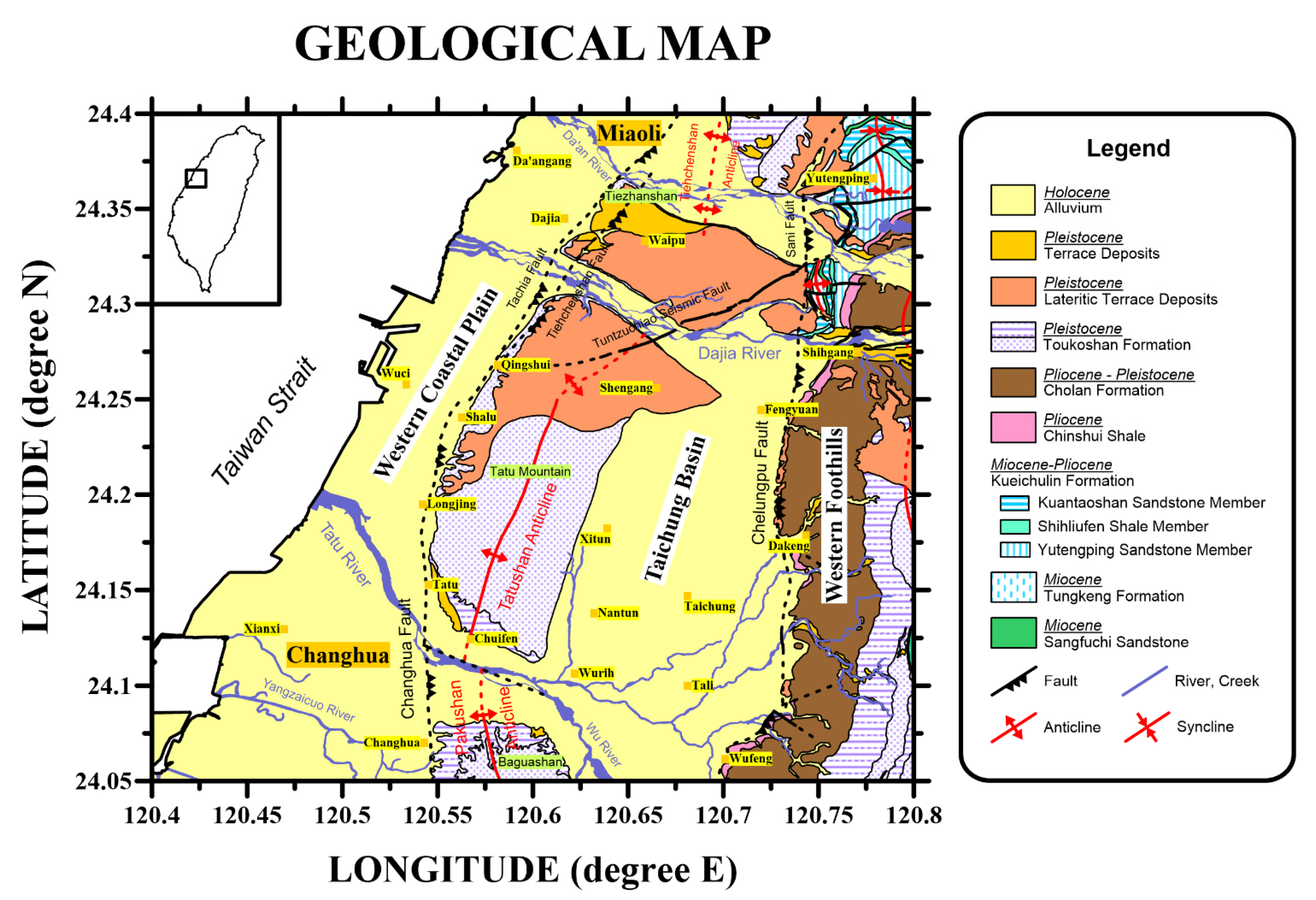
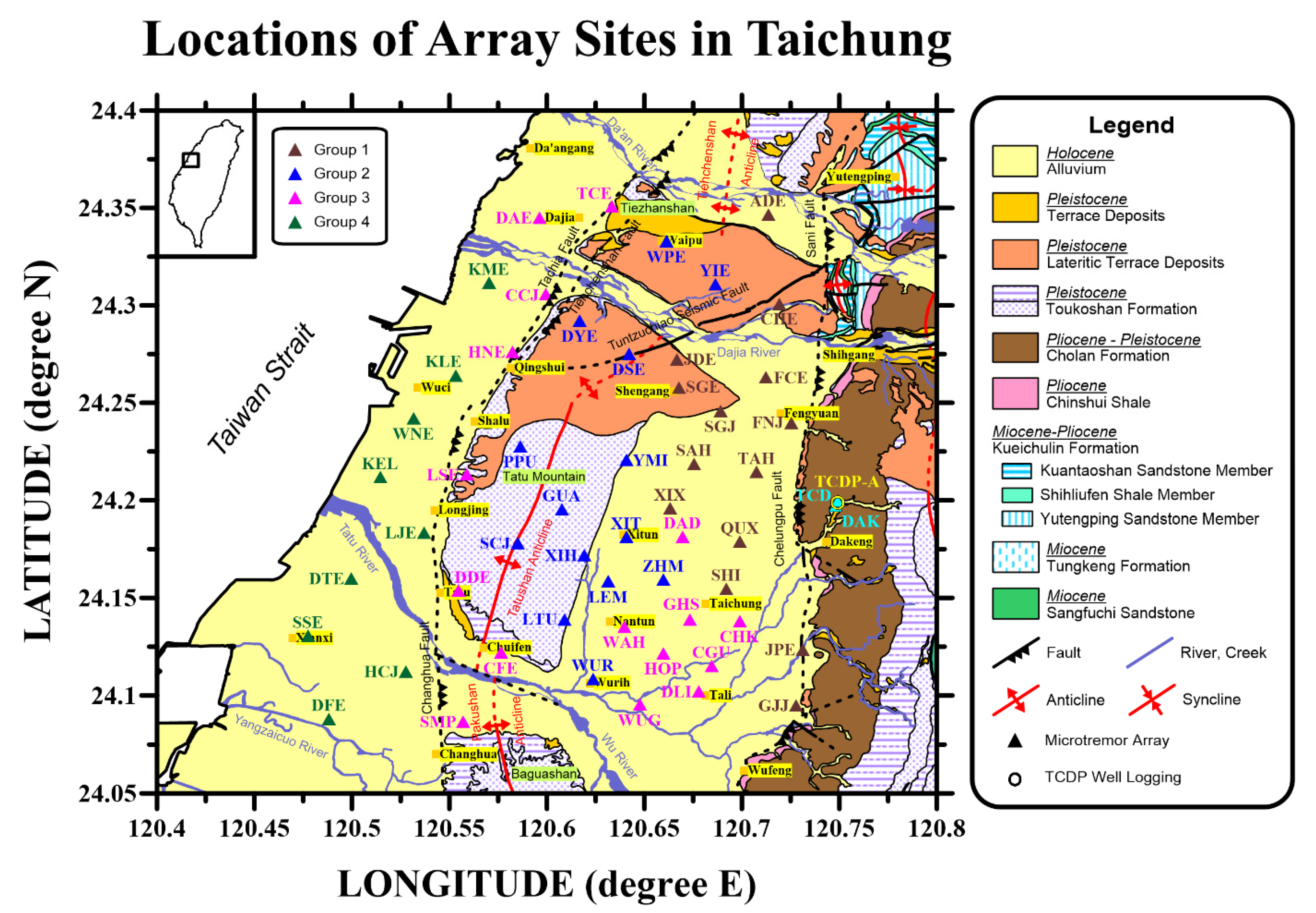
2. Sites and Data

The study area covered most of western Taichung and the neighboring regions in the west-central part of Taiwan (Figure 1). According to Ho and Chen [20], this area includes four geological regions: the foothills on the east (i.e., Western Foothills) and the coastal plain on the west (i.e., Western Coastal Plain) with the Taichung Basin and the Tatushan–Pakushan hills (i.e., Tatushan Anticline and Pakushan Anticline) between them (Figure 1). The Taichung Basin is a structural basin. The NS-trending Chelungpu Fault is the boundary fault between the foothills and the Taichung basin. The Tatushan–Pakushan hills (anticlines) separate the Western Coastal Plain from the Taichung piggyback basin because of the thrusting of the NS-trending Changhua Fault. The Tatushan–Pakushan hills, extending from the Dajia River (in northern Taichung) to the Choshui River (in southern Changhua), are mainly composed of conglomerates of the upper Toukoshan Formation. However, the thick-bedded sandstones, beneath the conglomerates in stratigraphic sequence, are only exposed in the area near the Tatu River. Widespread alluvium, which consists of gravel, sand, and clay, covers the Taichung Basin and the coastal plain [20].

In the study area, we performed microtremor array measurements at 53 sites. These sites covered most of western Taichung and most lie on alluvium (Figure 2). The distances between neighboring sites were between 2 and 5 km. At each site, microtremor arrays of two sizes (small [S] and large [L]) were used for measurements. At each array, 10 stations were deployed in the form of 3 triangles of varying apertures around the center station. Here, the site DTE on the Western Coastal Plain is employed as an example. Figure 3 exhibits the S- and L-array configurations at site DTE. The center station is fixed for the S and L arrays (min. and max. radii: 25 m and 100 m and 100 m and 400 m, respectively) at each site.

3. Methodology

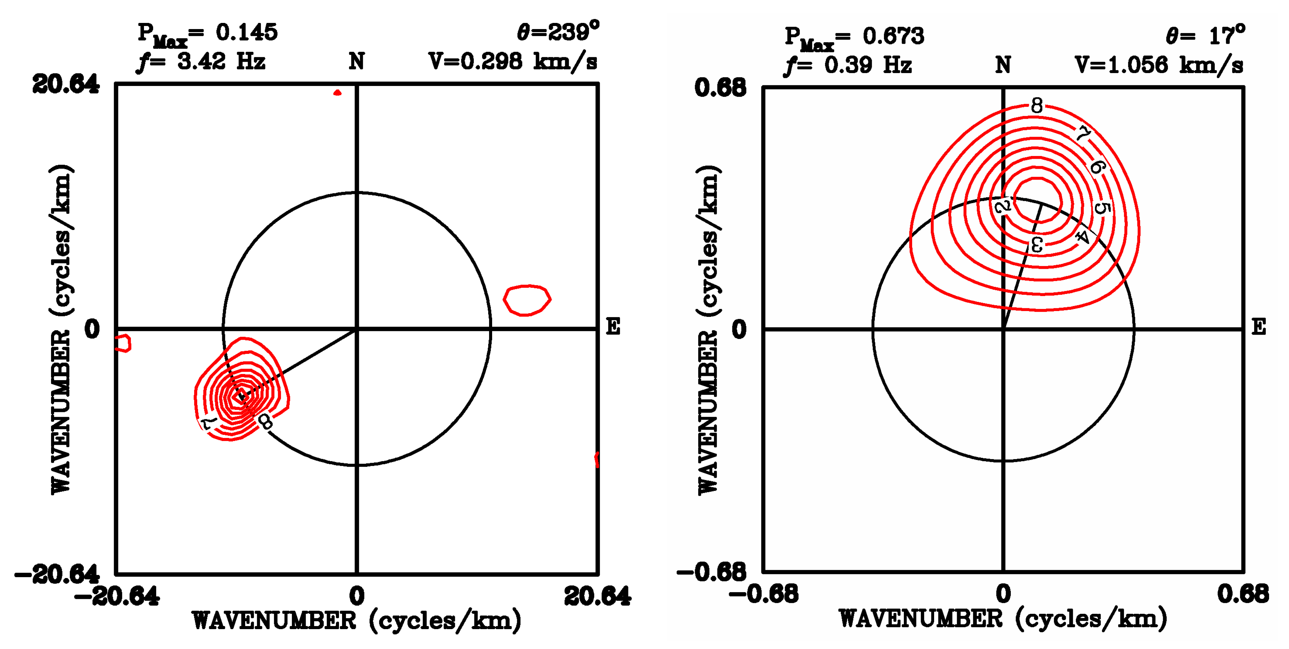
3.1. Frequency–Wavenumber Spectral Analysis Method

We adopted the frequency–wavenumber (F-K) method to analyze the array data of microtremors. The power spectrum P(f, k) at frequency f and vector wavenumber k for an array of N sensors using the maximum likelihood method (MLM; Capon [21]) can be expressed as

$$P\left(f,k\right)={\left[{\displaystyle \sum _{i,j=1}^N{\varphi }_{ij}^{-1}\left(f\right)\exp \left(i\overrightarrow{k}\cdot \overrightarrow{r_{ij}}\right)}\right]}^{-1}$$

(1)

where ${\varphi }_{ij}(f)$ represents the cross-power spectrum between the ith and jth sensors at frequency f; ${\varphi }_{ij}^{-1}(f)$ is the inverse of the coherence matrix ${\varphi }_{ij}(f)$; $\overrightarrow{r_{ij}}=\overrightarrow{r_j}-\overrightarrow{r_i}$ where $\overrightarrow{r_i}$ and $\overrightarrow{r_j}$ are the position vectors of the ith and jth sensors, respectively; and N is the number of sensors.

On the basis of the f–k spectrum, we searched for the peak power positions ($k_{x_0}$, $k_{y_0}$) in the wavenumber space and then calculated the phase velocity V as follows:

$$V=f/\sqrt{k_{x_0}^2+k_{y_0}^2}$$

(2)

3.2. Inversion of the S-Wave Velocity Structure

The discrete generalized inversion method was applied to determine the S-wave velocity structure. The problem was expressed as follows:

$$Y=AX$$

(3)

The vector Y of length n corresponds to the difference between the measured phase velocities and the calculated velocities for the initial model. The vector X of length m, which is the solution to be sought, corresponds to the first-order correction to an initial model.

In this study, we determined S-wave velocity structures by employing the surface-wave inversion technique [22]. For each site, we constructed an initial model with assigned values of thickness, S-wave velocity, and Poisson’s ratio for each layer. This initial model was assumed to be a half-space structure with an S-wave velocity that is the maximum phase velocity at the lowest used frequency divided by 0.92. According to the well-logging data, the Poisson’s ratio was estimated, and 0.4 was used for all layers. The total layer number was set to 80. The estimation of layer thickness was as follows: If a maximum frequency of 5 Hz and a phase velocity of approximately 450 m/s were used, the minimum wavelength was approximately 90 m. According to a rule of thumb, the highest resolution of thickness is about one-third of the minimum wavelength. Therefore, we could solve a layer with a thickness of 30 m. The depth resolution of the structure was determined according to the minimum frequency used and its corresponding phase velocity. For inversion, the damping value is adopted 1.0. We stopped the inversion process when the discrepancy of S-wave velocities between neighboring inversions was less than 0.001 km/s at each layer.

3.3. Examination of Analysis Methods

Between 2004 and 2006, the Taiwan Chelungpu Fault Drilling Project (TCDP) drilled a 2-km-deep hole (TCDP-A, Figure 2) 2.4 km east of the surface rupture of the Chi-Chi earthquake (near the town of Dakeng in Taichung municipality). Wu et al. [23] adopted geophysical well logs at depths between 500 and 1900 m to determine the physical properties of the fault zone and its neighboring damage areas. The well-logging data provided Wu and Huang [11] a suitable reference for inspecting the validity of the inverted velocity structures by using microtremor array measurements. Therefore, they conducted microtremor array measurements at two sites (DAK and TCD) close to the TCDP-A sites (Figure 2). In this study, the analysis methods and techniques used closely resembled those in [11]; thus we include Figure 4 (adopted from [11]) to certify that our inversion results (in Section 4) are reliable. In the figure, the S-wave velocity estimated from the differential inversion technique [22] gradually increases from 1.52 km/s at the depth of 585 m to 2.22 km/s at the depth of 1710 m. This velocity structure is similar to that from the well-logging data, which ranged from 1.4 km/s at the depth of 597 m to 2.98 km/s at the depth of 1705 m. This figure also displays the depth function (blue line) of the S-wave velocity, which is the regression result of the TCDP well-logging data at depths between 494 m and 1707 m in [24]. These results reveal that the S-wave velocity structures (black lines) estimated from microtremor array measurements were consistent with the depth function results. Therefore, the inversion velocity structures are reasonable and reliable. This also indicates that microtremor array measurement is a suitable approach for estimating deep or shallow S-wave velocity structures.

4. Results and Discussion

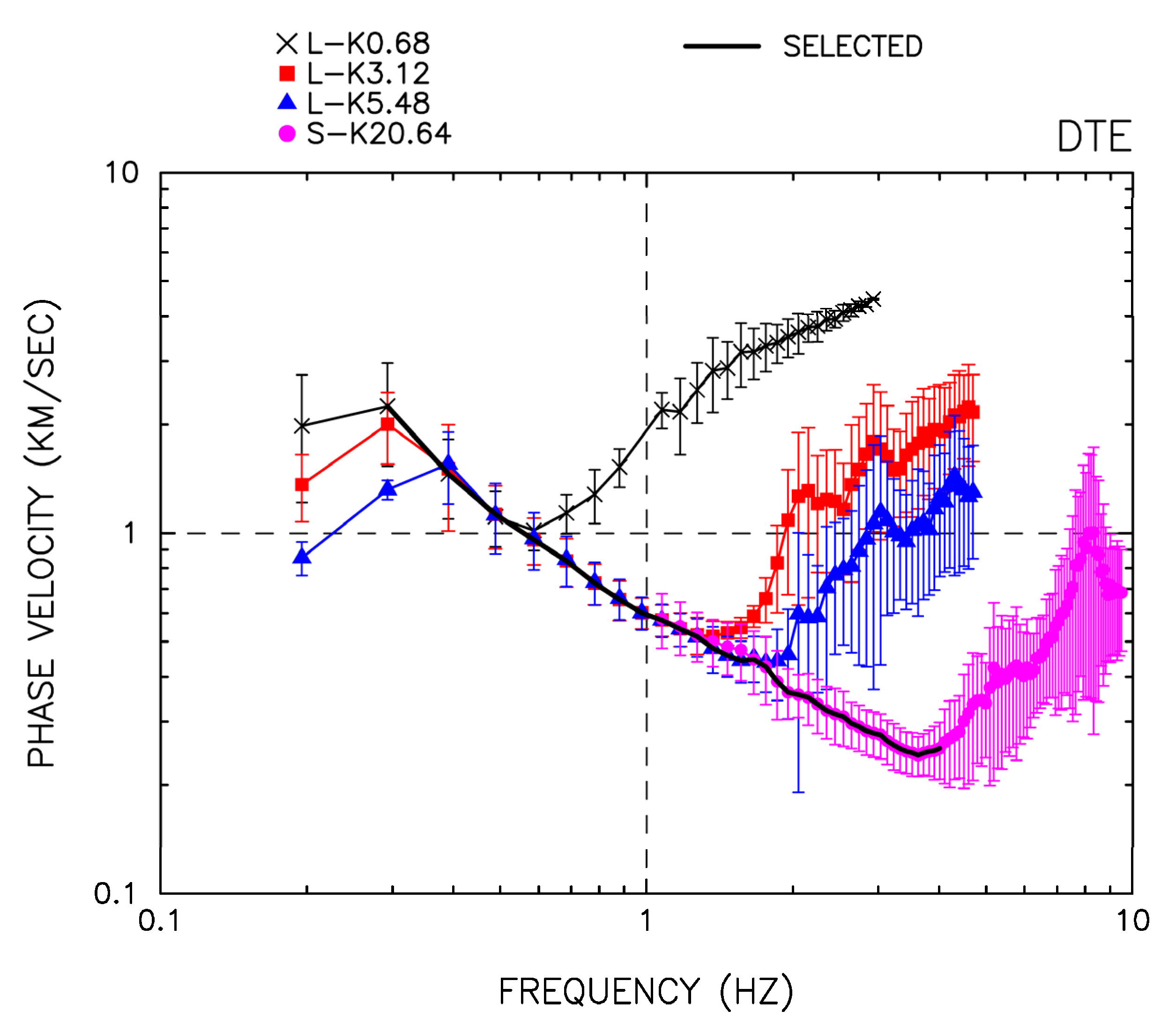
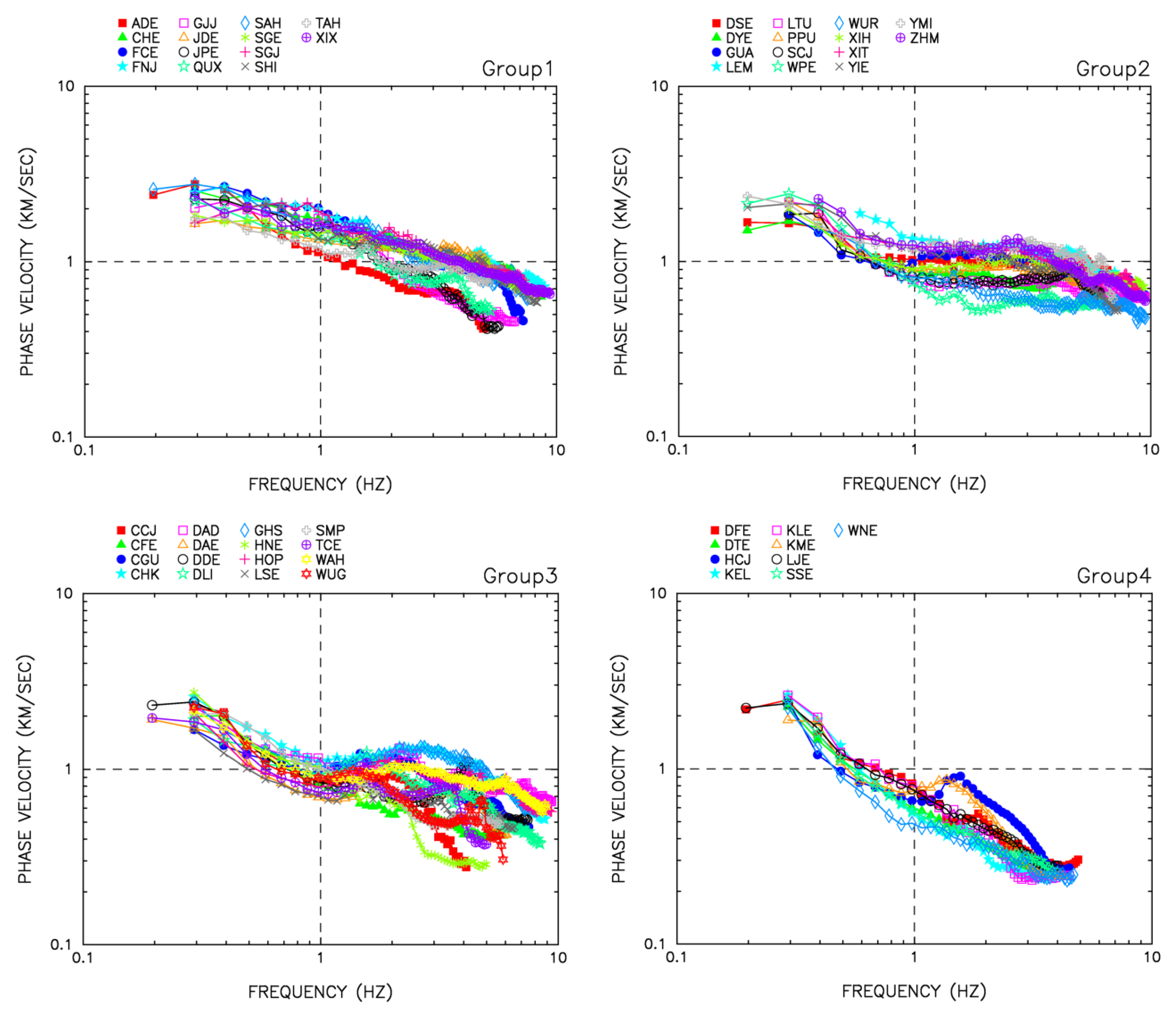
4.1. F-K Analysis of the Microtremor Array Data

We first divided the observed vertical-component recordings into multiple time segments by overlapping one-half of each window length. The window length was 20.48 s for S-array recordings and 40.96 s for L-array recordings. We inspected the data quality of recordings and eliminated certain segments contaminated by human activity and instrument noise. Subsequently, we calculated the phase velocities of the Rayleigh wave by using the FK method based on the MLM [21].

Figure 5 depicts the f–k spectra from the MLM using the microtremor data observed at site DTE. We calculated the f–k spectra at 51 × 51 grid points at each frequency. This figure displays the f–k spectra at 3.42 Hz (the left panel) and 0.39 Hz (the right panel) from the recordings generated by the S and L arrays, respectively. The propagation direction ($\theta$) was measured clockwise from north in degrees. For the two frequencies, the propagation directions were approximately 239° and 17°, respectively. The phase velocity (V) in km/s can be estimated from the maximum peak in the f–k spectrum. Since we identified the maximum peaks within the wavenumber windows that we set beforehand, the minimum phase velocities were limited, whereas the maximum phase velocities were not.

Figure 6 illustrates the estimated phase velocities at site DTE. The symbols represent the observed results from the different size arrays and K values. The observed phase velocities were selected by following the sequence of the L (0.29 Hz ≤ f ≤ 1.56 Hz) and S arrays (1.66 Hz ≤ f ≤ 4.0 Hz) from low to high frequencies. The results of the L-array measurements were stable at lower frequencies, whereas those of the S-array measurements were stable at higher frequencies.

Figure 7 depicts the dispersion curves of phase velocities obtained from recordings observed at all 53 sites. The estimated phase velocities varied between sites. Similar dispersion curves were categorized in the same group according to their amplitude and shape, yielding four groups. The Group 1 sites (14 sites) had the highest phase velocities, whereas those of Group 4 (9 sites) had the lowest phase velocities. The phase velocities of Groups 2 (14 sites) and 3 (16 sites) were between those of Groups 1 and 4. The sites illustrated in Figure 2 are color-coded with triangles according to this classification scheme. The sites of Group 4 (green triangles) appear on the Western Coastal Plain, whereas the sites of Group 3 (pink triangles) are distributed along the Changhua Fault and the southern Taichung Basin (i.e., old Taichung City). The sites of Group 2 (blue triangles) are on the Tatushan Anticline and the area north of it (which contain lateritic terrace deposits and terrace deposits). The sites of Group 1 (brown triangles) are on the northern Taichung Basin and near to or along the Chelungpu Fault (the eastern side). Furthermore, at most sites of Groups 2 and 3, the observed phase velocities were almost flat and were approximately 800–1300 m/s at frequencies between 0.6 and 2 Hz.

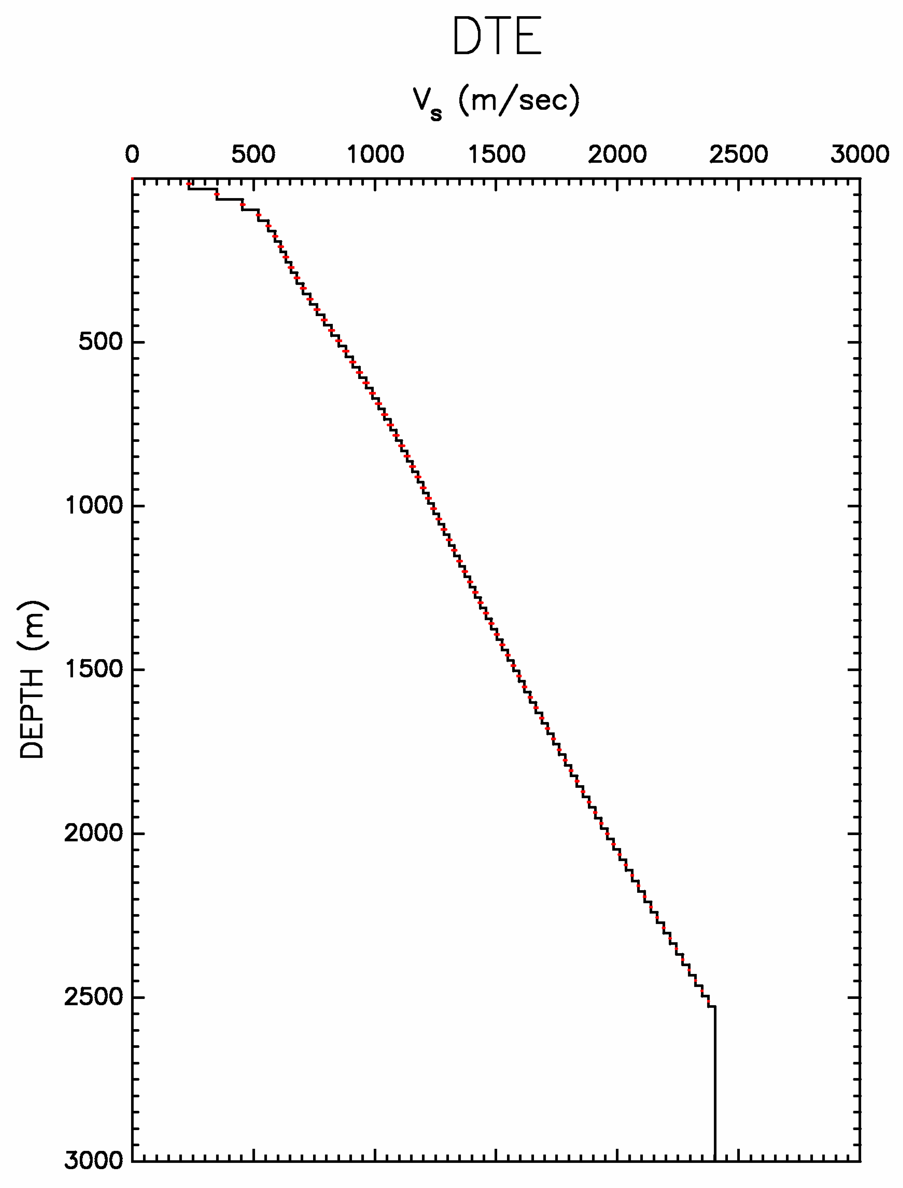
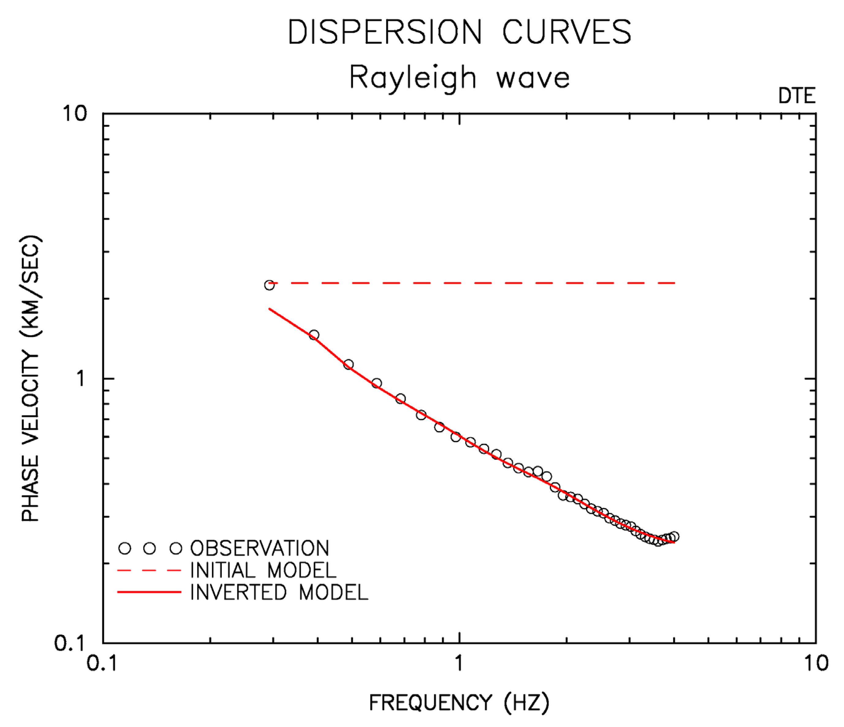
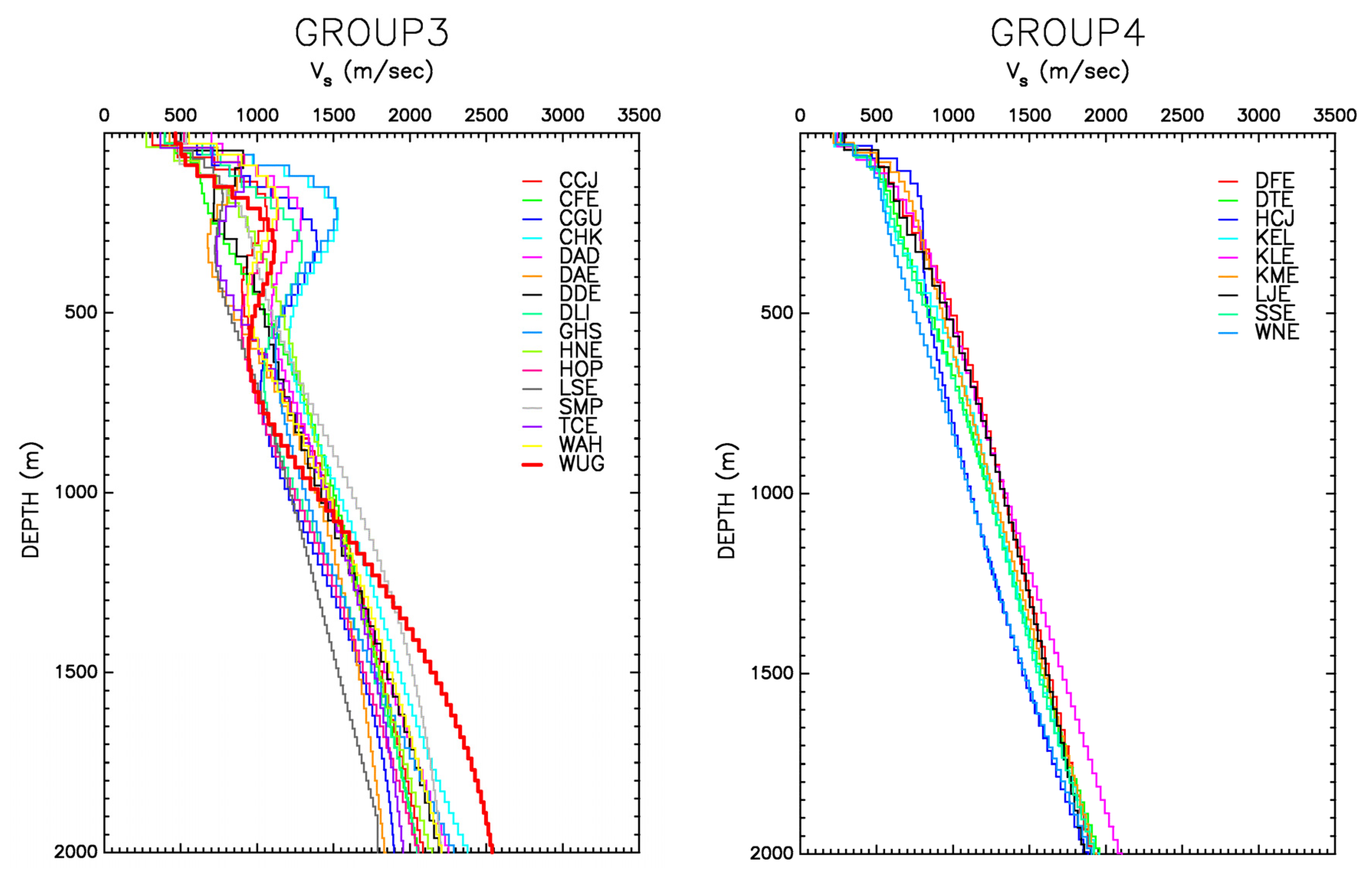
4.2. Inversion of the S-Wave Velocity Structure

On the basis of the results of the dispersion curves (Figure 7), we calculated S-wave velocity structures by using Herrmann’s inversion technique [22]. Figure 8 depicts the estimated S-wave velocity structures (~230–2350 m/s) at depths of 0–2500 m at site DTE. The inverted S-wave velocity gradually increased with depth. Figure 9 depicts the observed (open circles) and calculated (red lines) phase velocities for the initial (red dashed lines) and inverted (red solid line) S-wave velocity structures at site DTE. The theoretical phase velocities (red solid line) from the inverted results (Figure 8) closely resemble the observed phase velocities (open circles).

Figure 10 displays the one-dimensional (1D) S-wave velocity structures at depths of 0–2000 m estimated using the surface-wave (differential) inversion technique at all 53 sites. These structures were divided into four groups following the classification scheme in Figure 7. At most sites of Groups 2 and 3, the shallow S-wave structures have a convex shape at depths of 0–500 m. This means that they have a high-velocity zone at shallow depths. This result is consistent with the phenomenon that the observed phase velocities were almost flat in frequencies between 0.6 and 2 Hz. Moreover, if we assume the S-wave velocity of the Tertiary basement to be 1500 m/s, the Quaternary alluvial thickness overlying the bedrock is between 270 m (i.e., SGJ) and 1550 m (i.e., WNE) in the Taichung area. Among these sites, site FNJ (near the Chelungpu Fault) has the highest S-wave velocities and thinnest alluvium, whereas the lowest S-wave velocities and thickest alluvium occur at site WNE (on the Western Coastal Plain).

To elucidate the variation of the shallow S-wave velocities in the Taichung area, we include contour maps of the S-wave velocities at depths of 50–1800 m in Figure 11, based on the results of Figure 10. The contour maps indicate the presence of lateral heterogeneity and that velocities change with depth. The results are as follows:

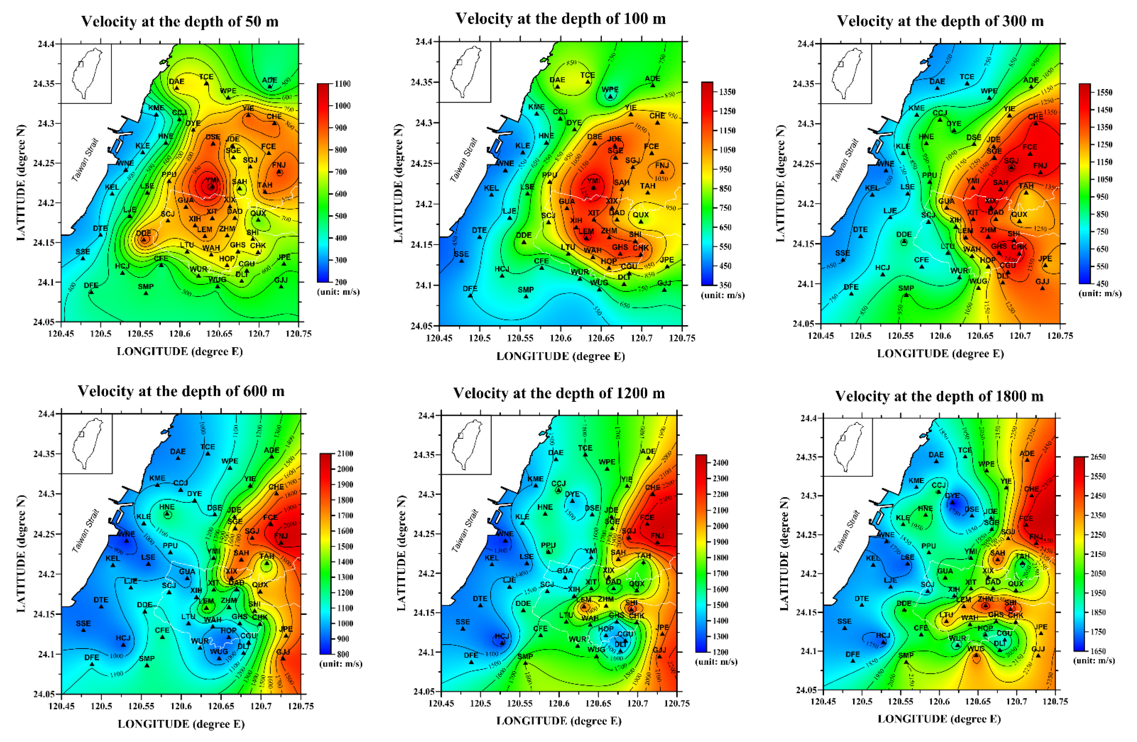
(1)

Depths of 50–300 m: The highest velocities appear at the central part (YMI), whereas the lowest velocities appear at the western part (WNE). The area with the highest S-wave velocities gradually shifts from the central part (YMI) to the northeastern part (SGJ) as depth increases.

(2)

Depths of 300–600 m: The area with the highest S-wave velocities gradually shifts from the central part (SGJ) to the eastern part (FNJ), which is near the Chelungpu Fault, as depth increases. The lower velocities still appear at the western part (WNE).

(3)

Depths of 600–1200 m: The highest velocities appear at the eastern part (FNJ, FCE), whereas the lower velocities appear at the western (WNE) and southwestern (HCJ) parts.

(4)

Depths of 1200–1800 m: The highest velocities remain at the eastern part (FNJ, FCE). The second highest velocity zone appears at the area near sites SHI and ZHM. Similarly, the western part (WNE, HCJ) still exhibits the lowest velocities.

Overall, the S-wave velocities gradually decrease from the east to the west as depths increase between 0 and 1800 m.

To clarify depth variations at the same velocity, a depth-contour map (upper panel) and 3D depth structure (lower panel) at a velocity of 1000 m/s were drawn (Figure 12). The depths are between 50 m (e.g., YMI, at the central part) and 850 m (e.g., WNE, at the western part). The shallowest depths appear at the central and eastern parts, whereas the deepest depths appear at the western part. Figure 13 displays the variations of the depths of the Tertiary basement, whose S-wave velocity is assumed to be 1500 m/s in the Taichung area. The depths of the bedrock range from 250 m (e.g., FCE and FNJ, at the eastern part) to 1550 m (e.g., WNE and HCJ, at the western part). The deepest alluvium appears at the western part of the area, whereas the shallowest alluvium appears at the eastern part. The depth of the alluvium gradually increases from the east to the west. Our results are consistent with the known geology of the Taichung area. These differences in bedrock depth indicate that estimated seismic amplification for thicker sediment will be higher than for thinner sediment.

5. Conclusions

In this study, we investigated shallow S-wave velocity structures (approximately 0–2000 m) beneath Taichung municipality in the west-central part of Taiwan. To accomplish this aim, we performed microtremor array measurements at 53 sites in the Taichung area. At each site, two different-sized arrays were deployed, and their radii ranged from 25 m to 400 m. At each array, 10 stations were used and deployed in the form of 3 triangles of differing apertures around a center station.

For the analysis of microtremor array recordings, we first adopted the FK spectrum method to estimate the phase velocities of Rayleigh waves at each site. Therefore, we obtained dispersion curves at all 53 sites. The calculated phase velocities varied between sites. The acquired dispersion curves illustrate that the softer sites (e.g., WNE, western coastal plain) had lower phase velocities than the harder sites (e.g., FNJ, near the Chelungpu Fault). We categorized similar dispersion curves into groups according to their amplitude and shapes. They were roughly divided into four groups. The sites of Group 1 (near or along the Chelungpu Fault) had the highest phase velocities, whereas those of Group 4 (at the western coastal plain) had the lowest values. The phase velocities of Groups 2 and 3 were between those of Groups 1 and 4.

Furthermore, with reference to the dispersion curves, we calculated S-wave velocity structures by using the surface-wave inversion method at all sites. According to the 1D velocity profile, among these sites, site FNJ (near the Chelungpu Fault) had the highest S-wave velocities and thinnest alluvium, whereas site WNE (on the Western Coastal Plain) had the lowest S-wave velocities and thickest alluvium. If we assume that the S-wave velocity of the Tertiary basement is 1500 m/s, the thicknesses of Quaternary sediments are between 270 m (i.e., SGJ, at the eastern side) and 1550 m (i.e., WNE, on the Western Coastal Plain) in the Taichung area.

To clarify the variations of V_S structures in the area, we sketched 2D and 3D maps based on the inversion results. According to the V_S-contour maps at different depths between 50 m and 1800 m, the lowest S-wave velocities were observed at the Western Coastal Plain, whereas the highest values appeared on the eastern side. The S-wave velocities gradually increased from the west to the east. According to the depth-contour map (Vs = 1500 m/s), the depths of the bedrock range from 250 m (e.g., FCE and FNJ, at the eastern part) to 1550 m (e.g., WNE and HCJ, at the western part). The thickness of the alluvium gradually increases from the east to the west. These results are consistent with the known geology of the Taichung area. These shallow S-wave velocity structures (0–2000 m) should be useful in future regional site-effect studies and ground-motion simulations or predictions.

References

- Horike, M. Inversion of phase velocity of long-period microtremors to the S-wave-velocity structure down to the basement in urbanized area. J. Phys. Earth 1985, 33, 59–96. [Google Scholar] [CrossRef] [Green Version]
- Central Geology Survey (2019) National Geological Data Warehouse, Central Geology Survey, the Ministry of Economic Affairs, Taipei, Taiwan. Available online: https://gis3.moeacgs.gov.tw/gwh/gsb97-1/sys8/t3/index1.cfm (accessed on 31 March 2020).
- Matsushima, T.; Okada, H. Determination of deep geological structures under urban areas using long-period microtremors. Butsuri-Tansa 1990, 43, 21–33. [Google Scholar]
- Kawase, H.; Satoh, T.; Iwata, T.; Irikura, K. S-wave velocity structures in the San Fernando and Santa Monica areas. In Proceedings of the 2nd International Symposium on Effects of Surface Geology on Seismic Motions, Yokohama, Japan, 1–3 December 1998; Volume 2, pp. 733–740. [Google Scholar]
- Satoh, T.; Kawase, H.; Iwata, T.; Higashi, S.; Sato, T.; Irikura, K.; Huang, H.C. Estimation of S-wave velocity structures in and around the Sendai basin, Japan, using array records of microtremors. Bull. Seism. Soc. Am. 2001, 91, 206–218. [Google Scholar] [CrossRef]
- Satoh, T.; Kawase, H.; Iwata, T.; Higashi, S.; Sato, T.; Irikura, K.; Huang, H.C. S-wave velocity structure of the Taichung basin, Taiwan, estimated from array and single-station records of microtremors. Bull. Seism. Soc. Am. 2001, 91, 1267–1282. [Google Scholar] [CrossRef]
- Huang, H.C.; Wu, C.F. Estimation of S-wave velocity structures in the Chia-Yi City, Taiwan using array records of microtremors. Earth Planets Space 2006, 58, 1455–1462. [Google Scholar] [CrossRef] [Green Version]
- Lin, C.M.; Chang, T.M.; Huang, Y.C.; Chiang, H.J.; Kuo, C.H.; Wen, K.L. Shallow S-wave velocity structures in the Western Coastal Plain of Taiwan. Terr. Atmos. Ocean Sci. 2009, 20, 299–308. [Google Scholar] [CrossRef] [Green Version]
- Wu, C.F.; Huang, H.C. Estimation of shallow S-wave velocity structure in the Puli basin, Taiwan, using array measurements of microtremors. Earth Planets Space 2012, 64, 389–403. [Google Scholar] [CrossRef] [Green Version]
- Wu, C.F.; Huang, H.C. Near-surface shear-wave velocity structure of the Chiayi area, Taiwan. Bull. Seism. Soc. 2013, 103, 1154–1164. [Google Scholar] [CrossRef]
- Wu, C.F.; Huang, H.C. S-Wave Velocity Structure of the Taiwan Chelungpu-Fault Drilling Project (TCDP) Site Using Microtremor Array Measurements. Pure Appl. Geophys. 2015, 172, 2545–2556. [Google Scholar] [CrossRef]
- Wu, C.F.; Huang, H.C. Detection of a Fracture Zone Using Microtremor Array Measurement. Geophysics 2019, 84, B33–B40. [Google Scholar] [CrossRef]
- Huang, H.C.; Wu, C.F.; Lee, F.M.; Hwang, R.D. S-Wave Velocity Structures of the Taipei Basin, Taiwan, Using Microtremor Array Measurements. J. Asian Earth Sci. 2015, 101, 1–13. [Google Scholar] [CrossRef]
- Kuo, C.H.; Chen, C.T.; Lin, C.M.; Wen, K.L.; Huang, J.Y.; Chang, S.C. S-wave velocity structure and site effect parameters derived from microtremor arrays in the Western Plain of Taiwan. J. Asian Earth Sci. 2016, 128, 27–41. [Google Scholar] [CrossRef] [Green Version]
- Singh, A.P.; Shukla, A.; Kumar, M.R.; Thakkar, M.G. Characterizing surface geology, liquefaction potential, and maximum intensity in the Kachchh Seismic Zone, Western India, through microtremor analysis. Bull. Seism. Soc. Am. 2017, 107, 1277–1292. [Google Scholar] [CrossRef]
- Özmen, Ö.T.; Yamanaka, H.; Alkan, M.A.; Çeken, U.; Öztürk, T.; Sezen, A. Microtremor array measurements for shallow S-wave profiles at strong-motion stations in Hatay and Kahramanmaras Provinces, Southern Turkey. Bull. Seism. Soc. Am. 2017, 107, 445–455. [Google Scholar] [CrossRef]
- Ridwan, M.; Cummins, P.R.; Widiyantoro, S.; Irsyam, M. Site characterization using microtremor array and seismic hazard assessment for Jakarta, Indonesia. Bull. Seism. Soc. Am. 2019, 109, 2644–2657. [Google Scholar] [CrossRef]
- Ku, T.; Palanidoss, S.; Zhang, Y.; Moona, S.W.; Wei, X.; Huang, E.S.; Kumarasamy, J.; Goh, K.H. Practical configured microtremor array measurements (MAMs) for the geological investigation of underground space. Undergr. Space 2021, 6, 240–251. [Google Scholar] [CrossRef]
- Satoh, T.; Kawase, H.; Iwata, T.; Higashi, S.; Sato, T.; Huang, H.C. S-wave velocity structures of sediments estimated from array microtremor records and site responses in the near-fault Region of the 1999 Chi-Chi, Taiwan earthquake. J. Seismol. 2004, 8, 545–558. [Google Scholar]
- Ho, H.C.; Chen, M.M. Explanation Text of the Geological Map of Taiwan (Taichung, Scale 1:50,000, Sheet 24); Central Geological Survey, the Ministry of Economic Affairs: Taipei, Taiwan, 2000; p. 65, (In Chinese with English Summary). [Google Scholar]
- Capon, J. High-resolution frequency-wavenumber spectral analysis. Proc. IEEE 1969, 57, 1408–1419. [Google Scholar] [CrossRef] [Green Version]
- Herrmann, R.B. Computer Program in Seismology, Volume IV: Surface Wave Inversion; University of St. Louis: St. Louis, MO, USA, 1991; p. 58. [Google Scholar]
- Wu, H.Y.; Ma, K.F.; Zoback, M.; Boness, N.; Ito, H.; Hung, J.H.; Hickman, S. Stress orientations of Taiwan Chelungpu-Fault Drilling Project (TCDP) hole-A as observed from geophysical logs. Geophys. Res. Lett. 2007, 34, L01303. [Google Scholar] [CrossRef] [Green Version]
- Wang, J.H.; Hung, J.H.; Dong, J.J. Seismic velocities, density, porosity, and permeability measured at a deep hole penetrating the Chelungpu fault in central Taiwan. J. Asian Earth Sci. 2009, 36, 135–145. [Google Scholar] [CrossRef]
Publisher’s Note: MDPI stays neutral with regard to jurisdictional claims in published maps and institutional affiliations. |
© 2021 by the authors. Licensee MDPI, Basel, Switzerland. This article is an open access article distributed under the terms and conditions of the Creative Commons Attribution (CC BY) license (https://creativecommons.org/licenses/by/4.0/).
Share and Cite
Huang, H.-C.; Shih, T.-H.; Hsu, C.-T.; Wu, C.-F. Estimation of Shear-Wave Velocity Structures in Taichung, Taiwan, Using Array Measurements of Microtremors. Appl. Sci. 2022, 12, 170. https://doi.org/10.3390/app12010170
Huang H-C, Shih T-H, Hsu C-T, Wu C-F. Estimation of Shear-Wave Velocity Structures in Taichung, Taiwan, Using Array Measurements of Microtremors. Applied Sciences. 2022; 12(1):170. https://doi.org/10.3390/app12010170
Chicago/Turabian StyleHuang, Huey-Chu, Tien-Han Shih, Cheng-Ta Hsu, and Cheng-Feng Wu. 2022. "Estimation of Shear-Wave Velocity Structures in Taichung, Taiwan, Using Array Measurements of Microtremors" Applied Sciences 12, no. 1: 170. https://doi.org/10.3390/app12010170