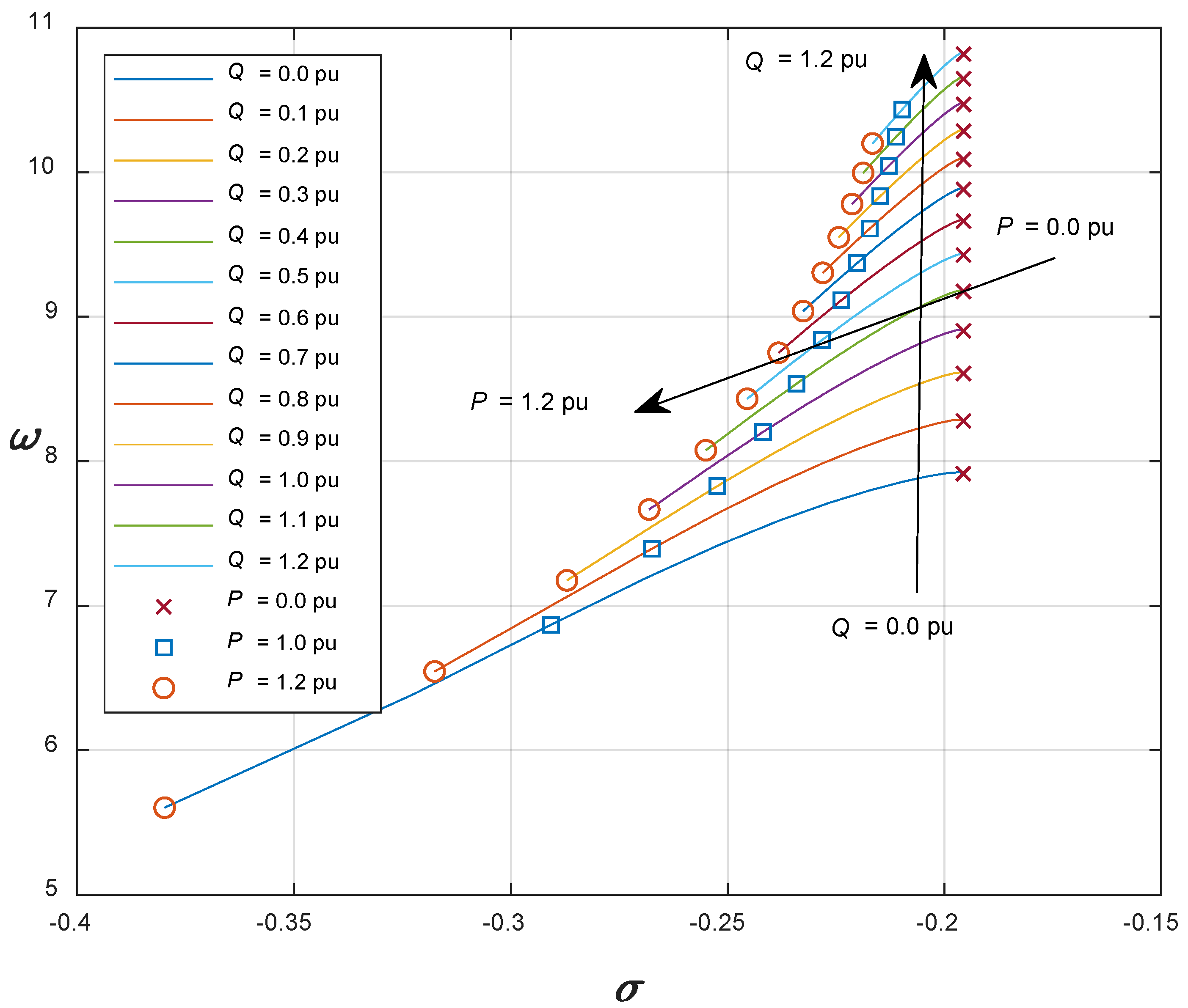
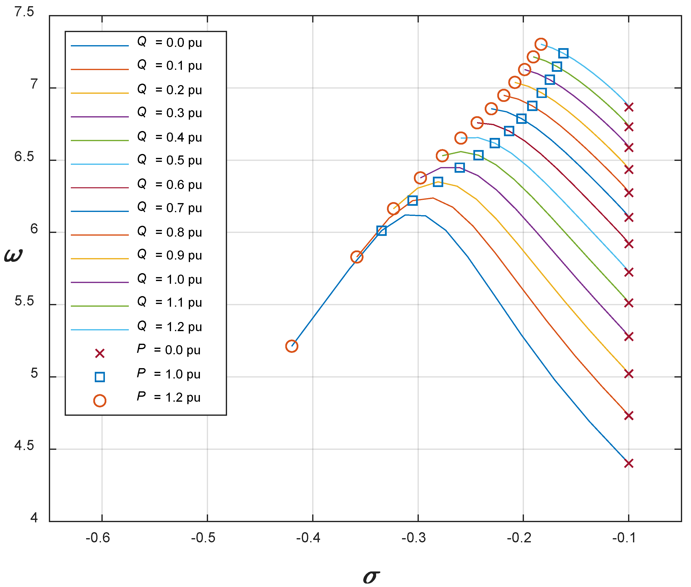
Figure 1.
Eigenvalue loci of local mode of 9-MVA hydro-type synchronous generator without AVR.
Figure 1.
Eigenvalue loci of local mode of 9-MVA hydro-type synchronous generator without AVR.
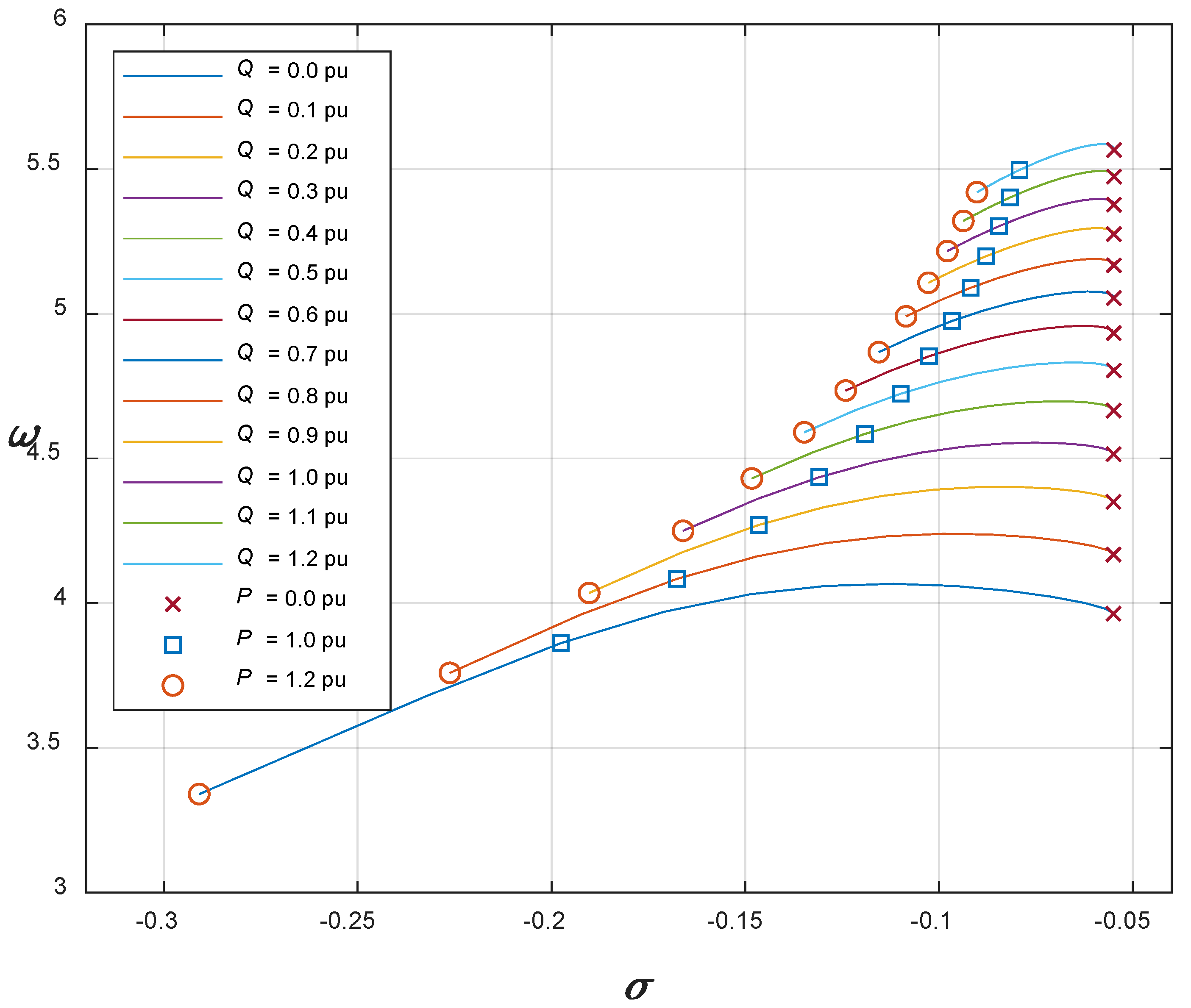
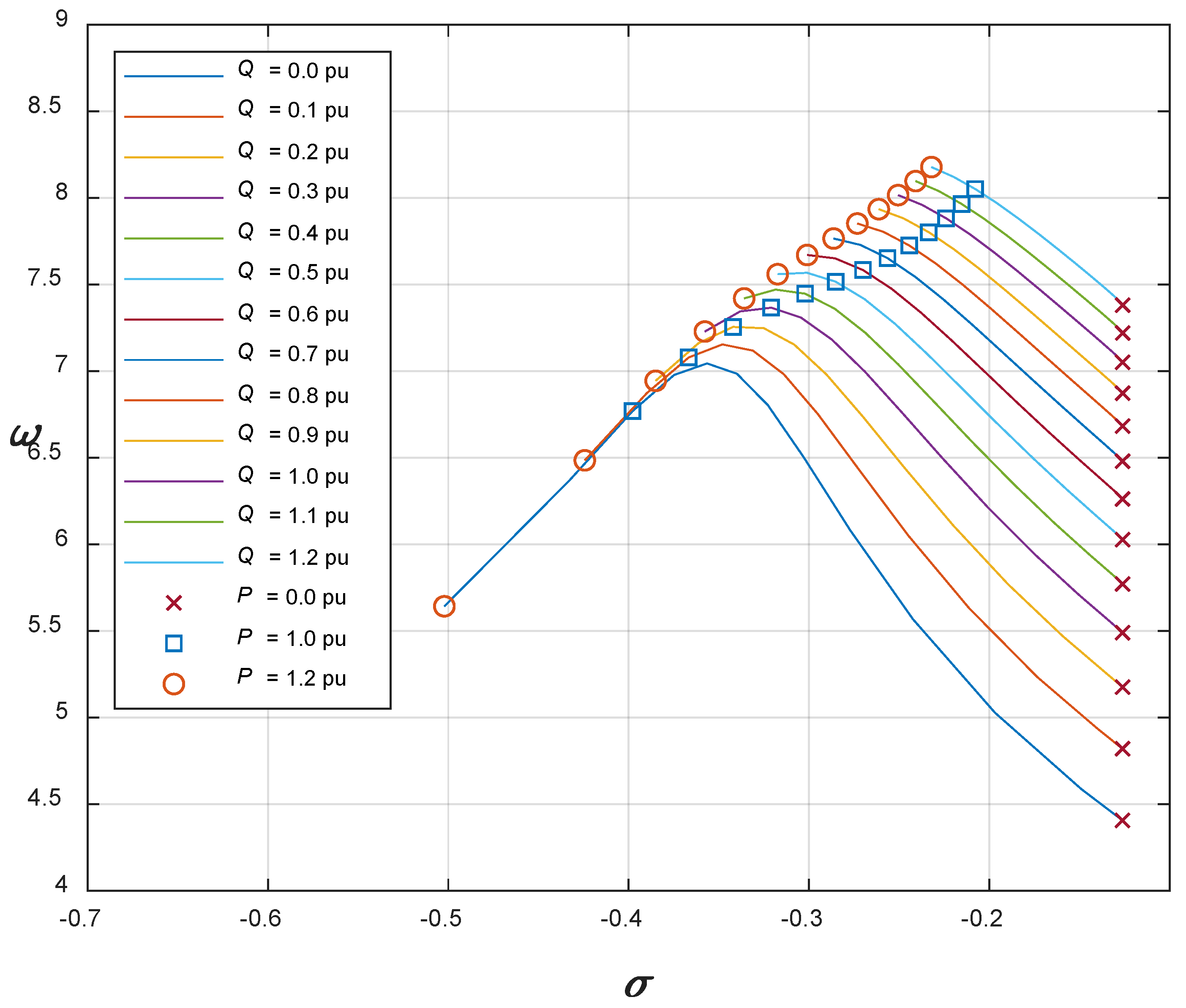
Figure 2.
Eigenvalue loci of local mode of 12-MVA hydro-type synchronous generator without AVR.
Figure 2.
Eigenvalue loci of local mode of 12-MVA hydro-type synchronous generator without AVR.
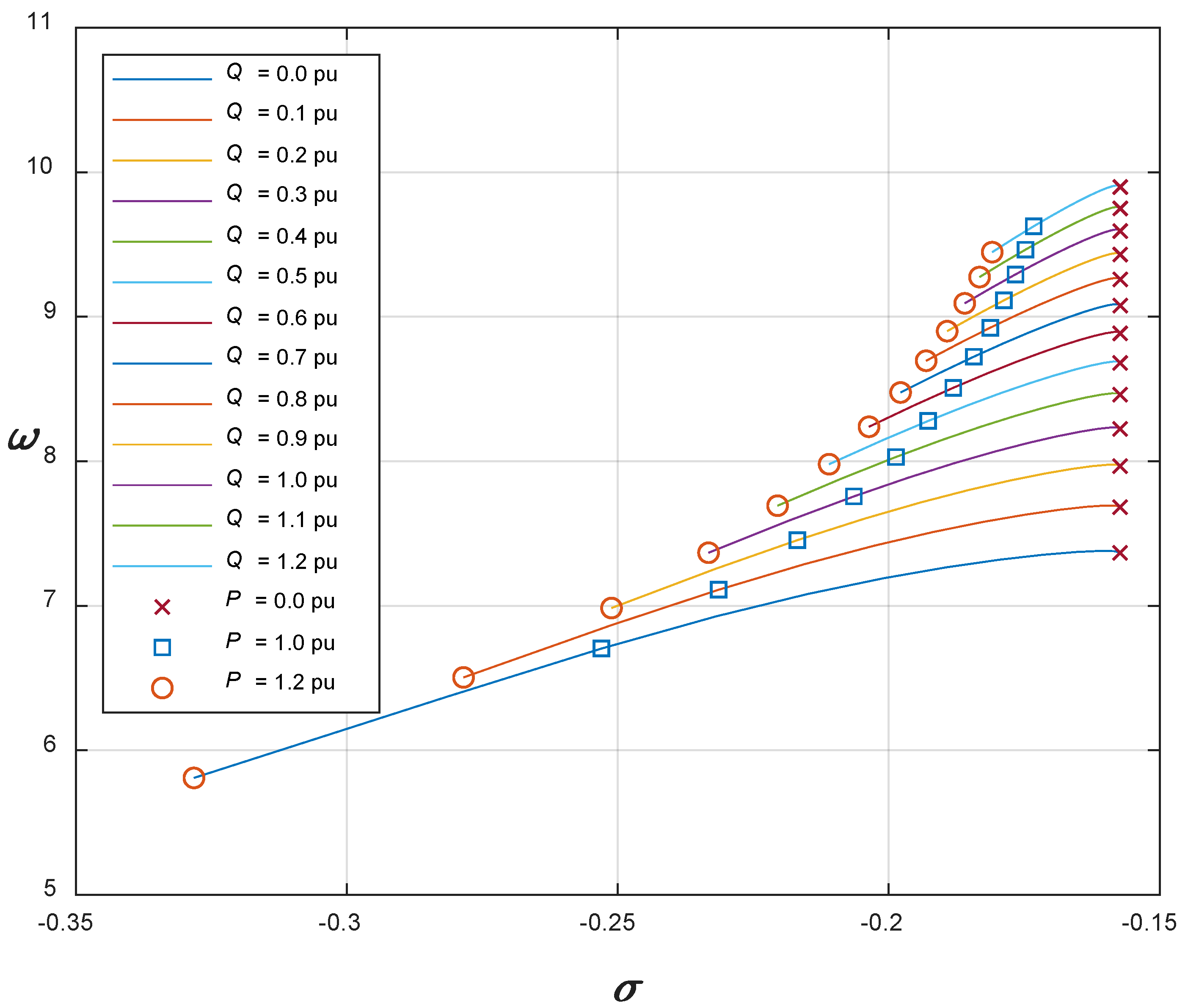
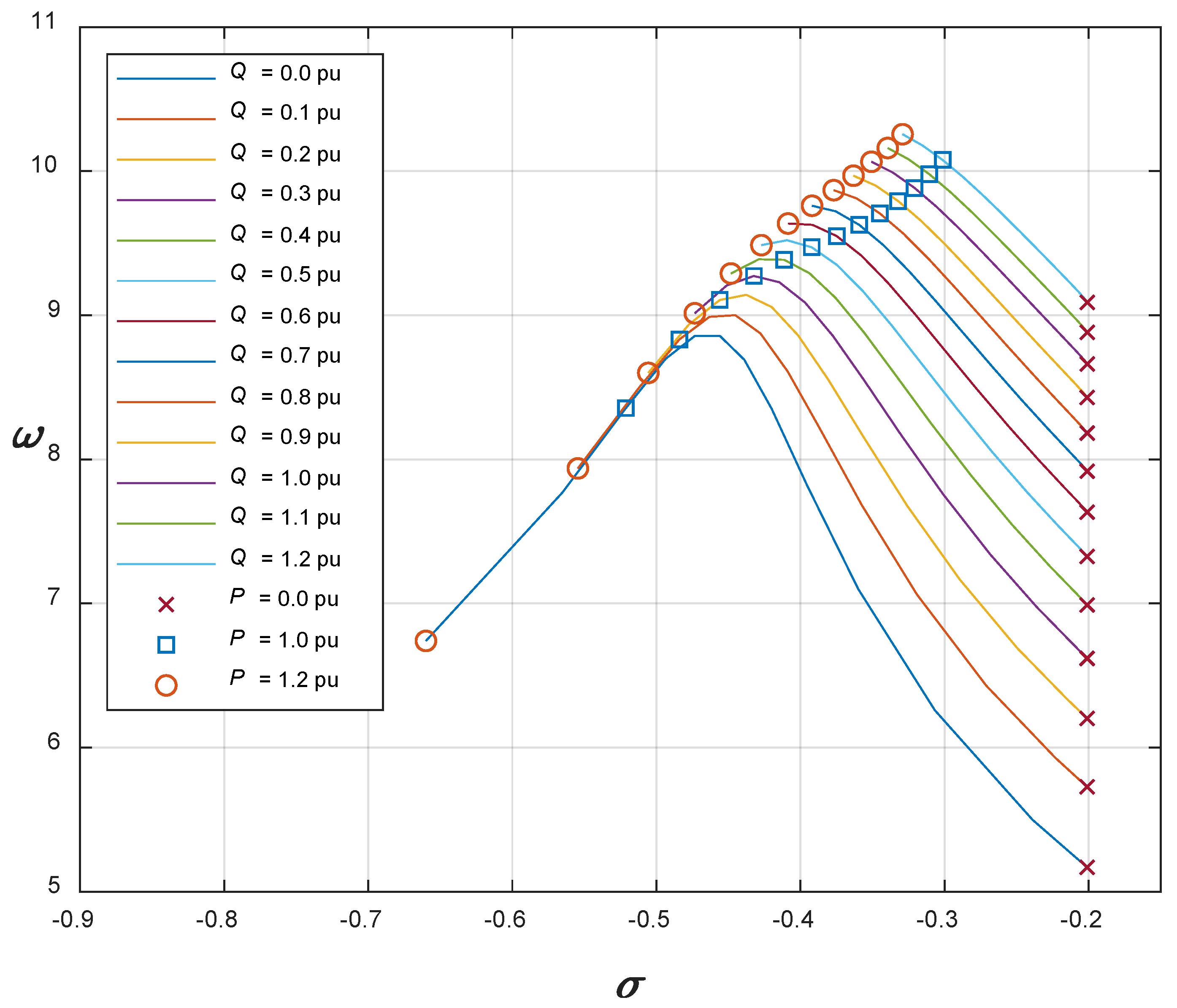
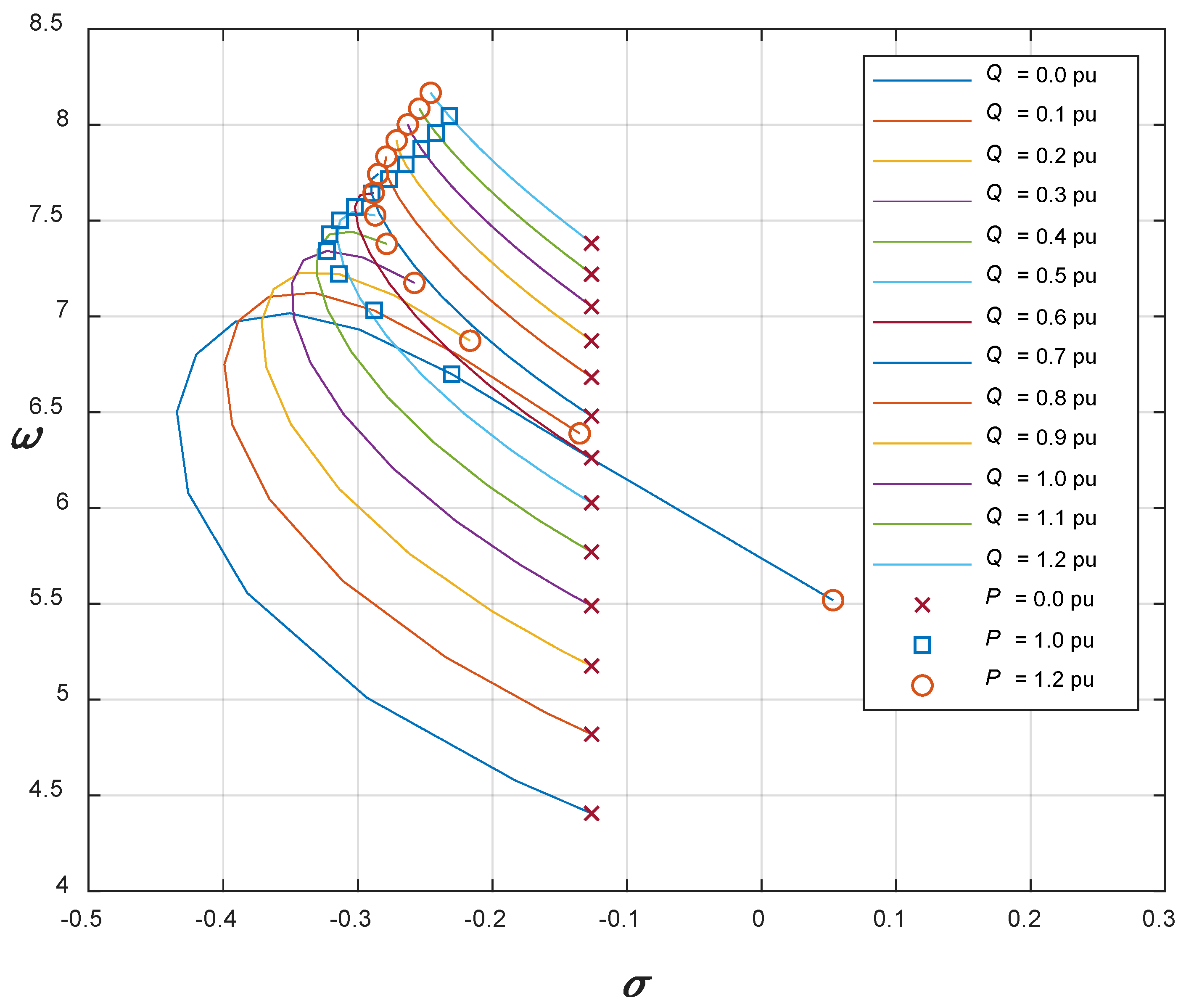
Figure 3.
Eigenvalue loci of local mode of 158-MVA hydro-type synchronous generator without AVR.
Figure 3.
Eigenvalue loci of local mode of 158-MVA hydro-type synchronous generator without AVR.
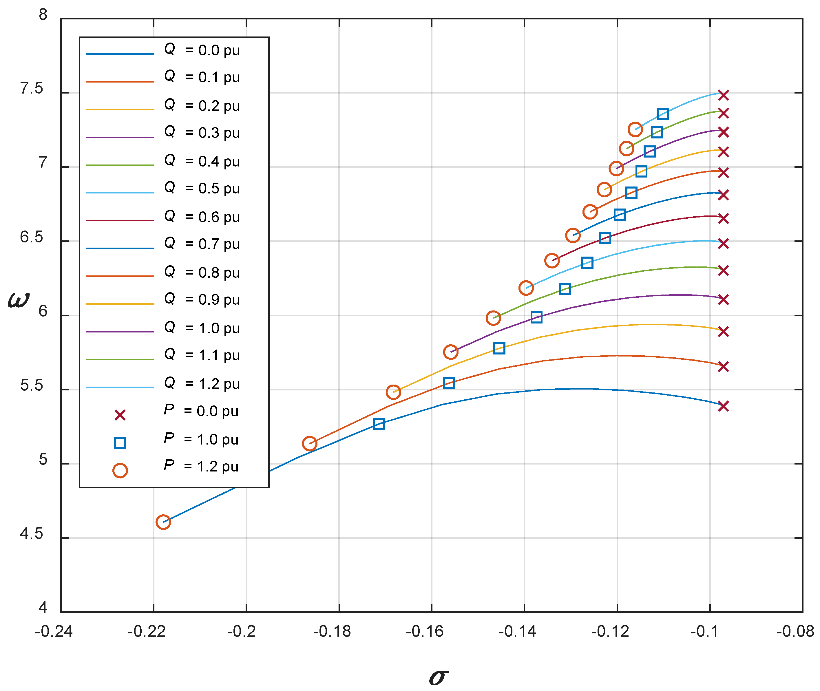
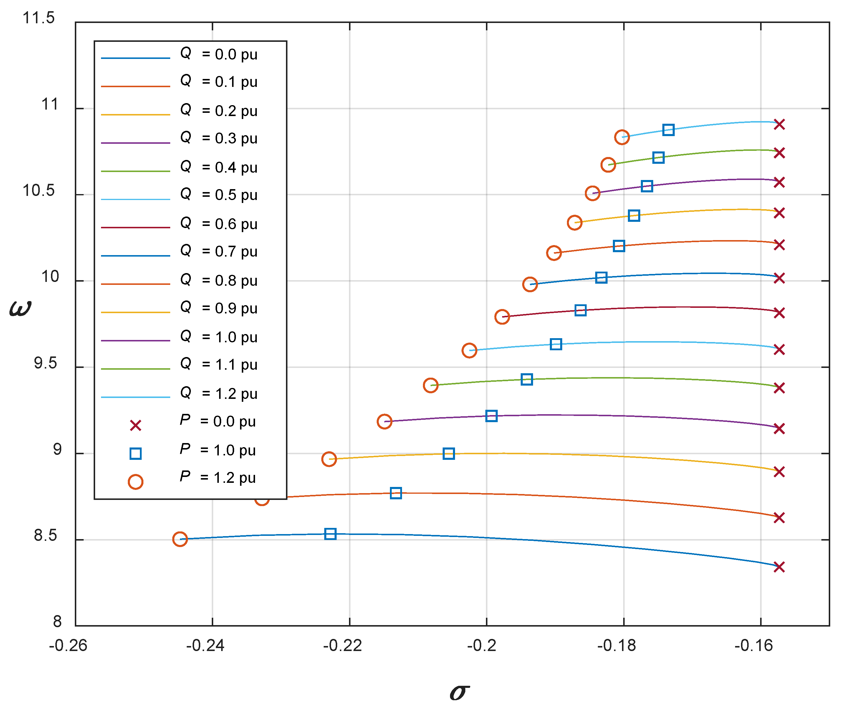
Figure 4.
Eigenvalue loci of local mode of 615-MVA hydro-type synchronous generator without AVR.
Figure 4.
Eigenvalue loci of local mode of 615-MVA hydro-type synchronous generator without AVR.
Figure 5.
Eigenvalue loci of local mode of 25-MVA turbo-type synchronous generator without AVR.
Figure 5.
Eigenvalue loci of local mode of 25-MVA turbo-type synchronous generator without AVR.
Figure 6.
Eigenvalue loci of local mode of 160-MVA turbo-type synchronous generator without AVR.
Figure 6.
Eigenvalue loci of local mode of 160-MVA turbo-type synchronous generator without AVR.
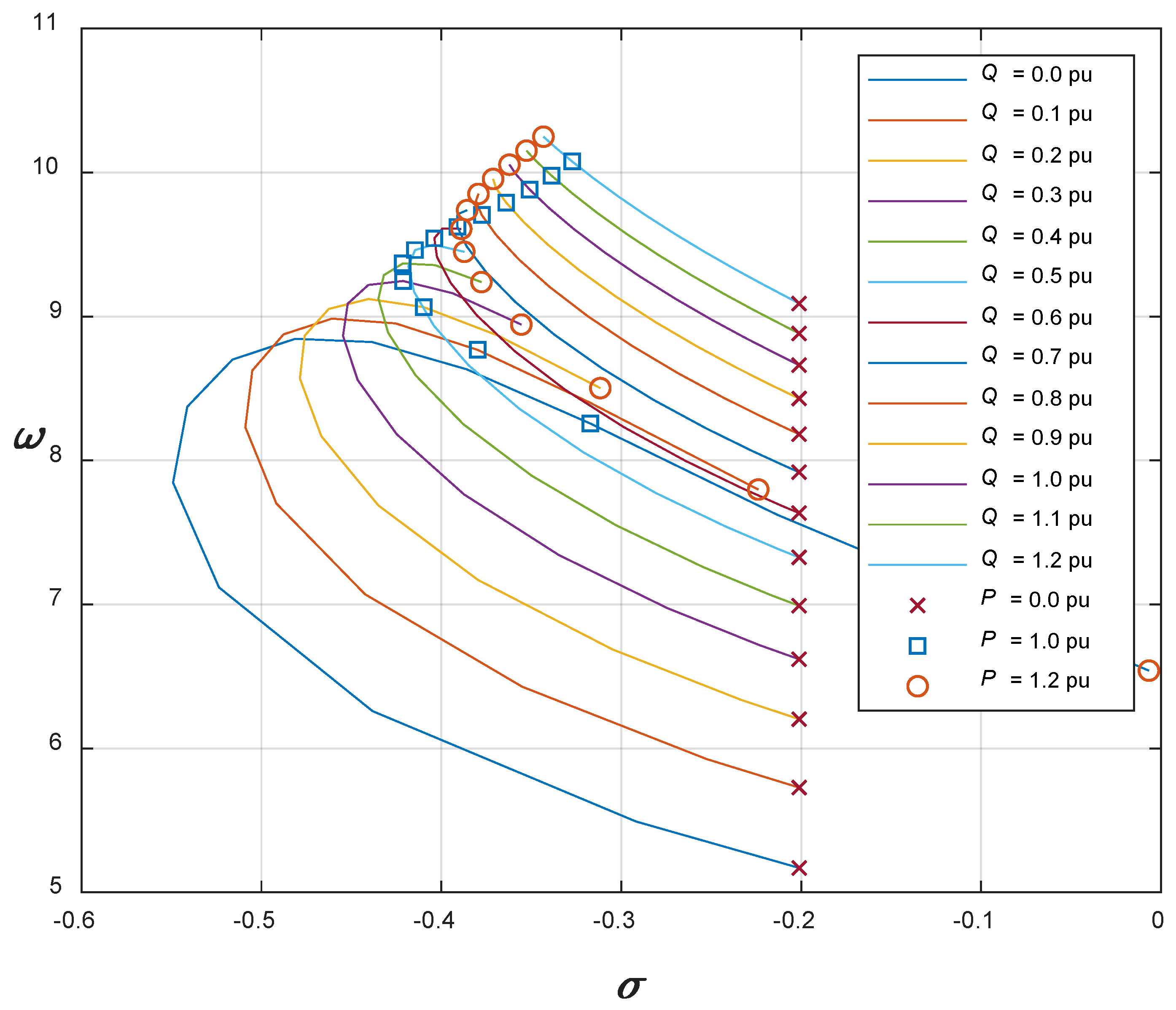
Figure 7.
Eigenvalue loci of local mode of 911-MVA turbo-type synchronous generator without AVR.
Figure 7.
Eigenvalue loci of local mode of 911-MVA turbo-type synchronous generator without AVR.
Figure 8.
Eigenvalue loci of local mode of a 158-MVA hydro-type synchronous generator where transmission line impedance was reduced to 50% of the nominal (real) impedance (comparable with
Figure 3).
Figure 8.
Eigenvalue loci of local mode of a 158-MVA hydro-type synchronous generator where transmission line impedance was reduced to 50% of the nominal (real) impedance (comparable with
Figure 3).
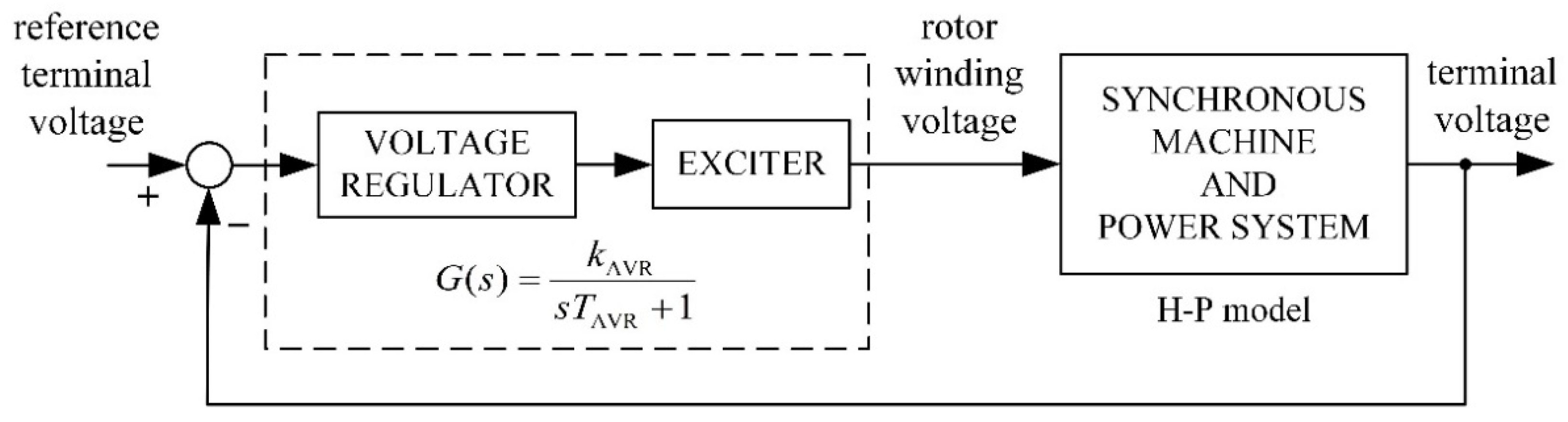
Figure 9.
Block diagram of the studied AVR system.
Figure 9.
Block diagram of the studied AVR system.
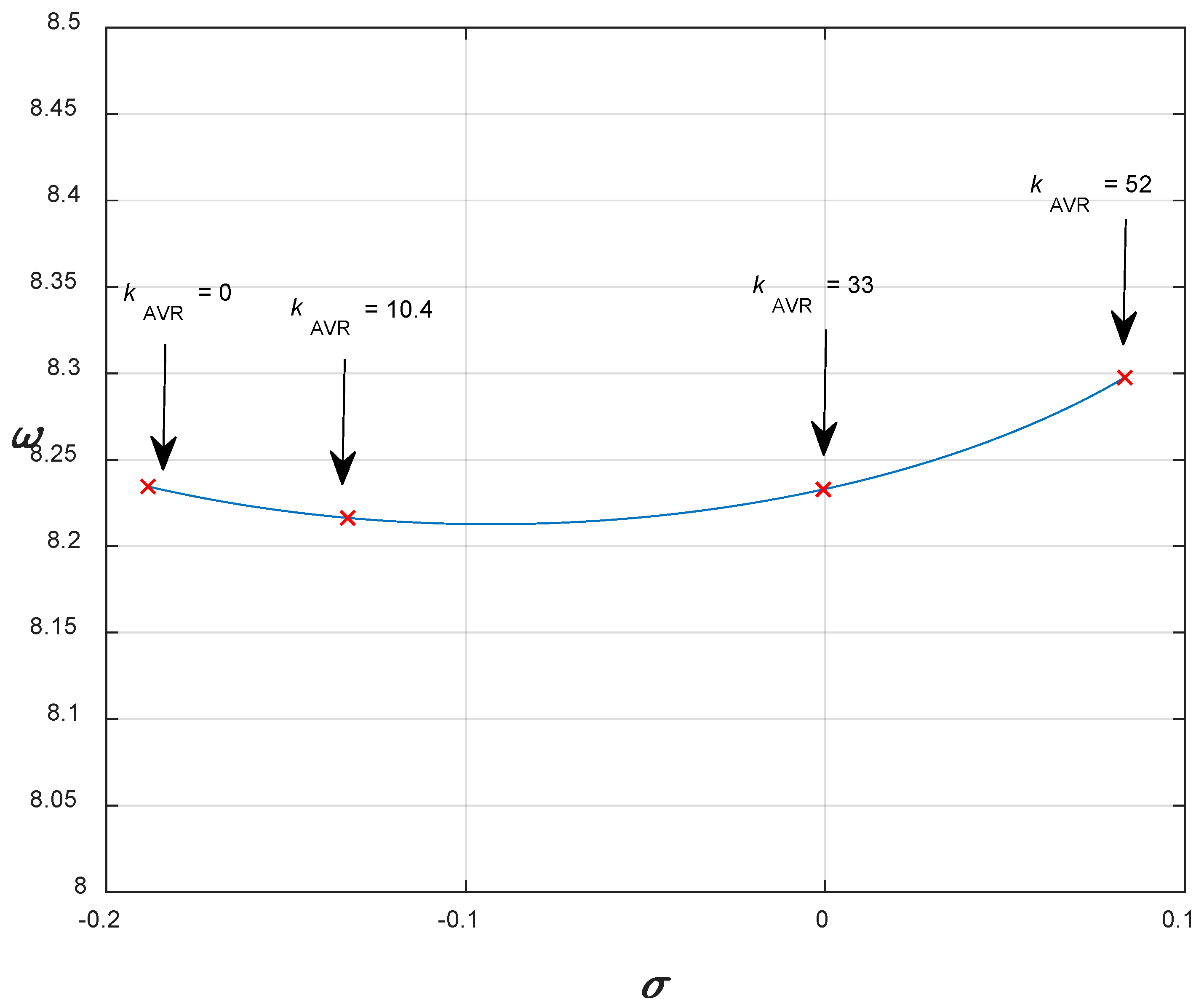
Figure 10.
Influence of exciter and AVR gain kAVR on the local mode eigenvalue of the hydro-generator with nominal power 158 MVA for nominal operating point S = 158 MVA, cos φ = 0.9.
Figure 10.
Influence of exciter and AVR gain kAVR on the local mode eigenvalue of the hydro-generator with nominal power 158 MVA for nominal operating point S = 158 MVA, cos φ = 0.9.
Figure 11.
Eigenvalue loci of the local mode of 9-MVA hydro-type synchronous generator with AVR.
Figure 11.
Eigenvalue loci of the local mode of 9-MVA hydro-type synchronous generator with AVR.
Figure 12.
Eigenvalue loci of the local mode of 12-MVA hydro-type synchronous generator with AVR.
Figure 12.
Eigenvalue loci of the local mode of 12-MVA hydro-type synchronous generator with AVR.
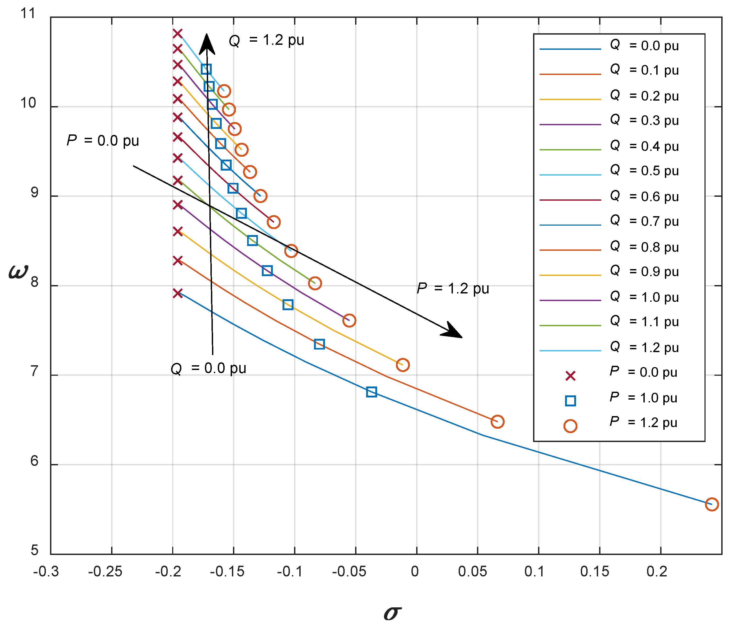
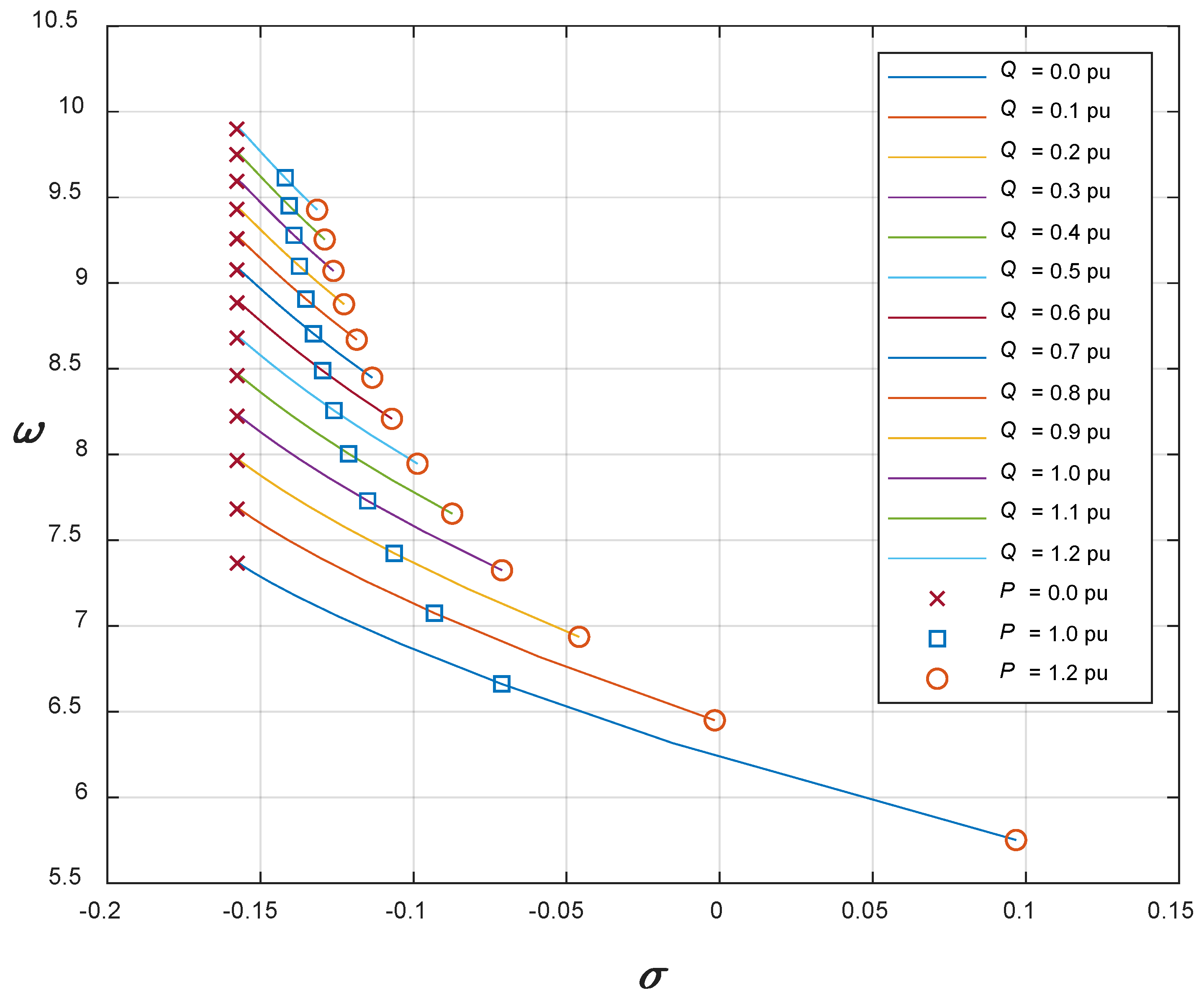
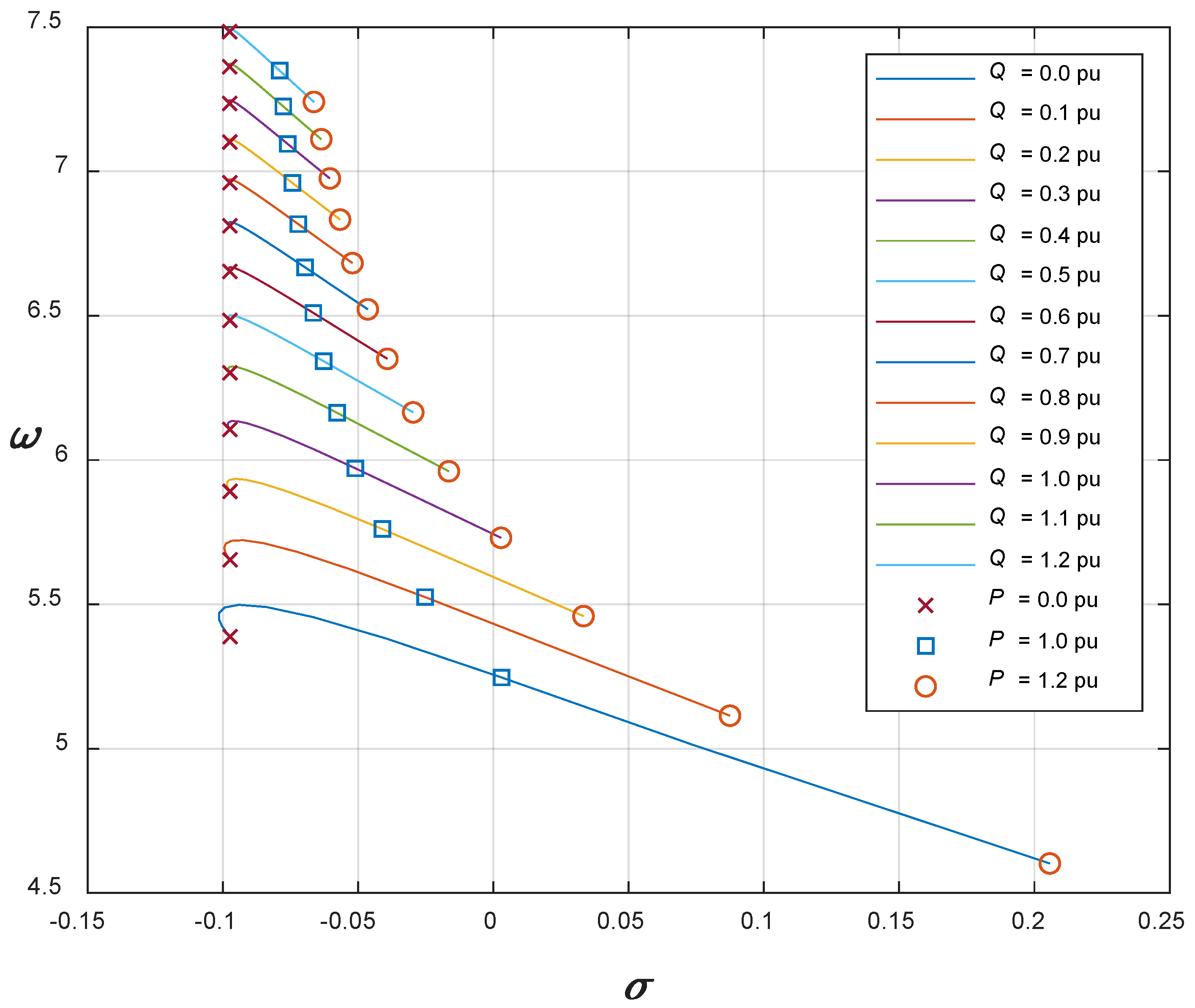
Figure 13.
Eigenvalue loci of the local mode of 158-MVA hydro-type synchronous generator with AVR.
Figure 13.
Eigenvalue loci of the local mode of 158-MVA hydro-type synchronous generator with AVR.
Figure 14.
Eigenvalue loci of the local mode of 615-MVA hydro-type synchronous generator with AVR.
Figure 14.
Eigenvalue loci of the local mode of 615-MVA hydro-type synchronous generator with AVR.
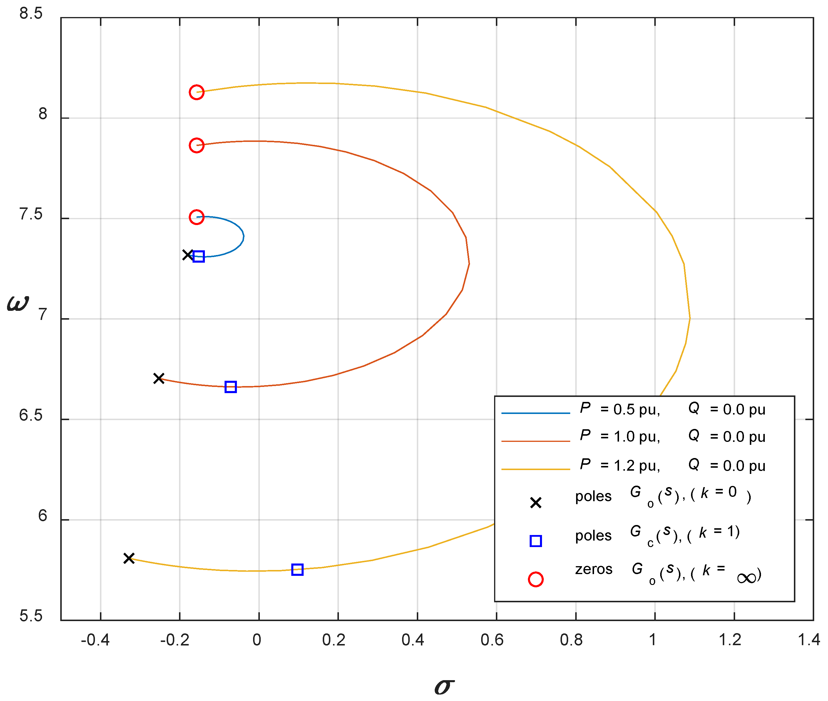
Figure 15.
Root locus diagrams of local mode eigenvalue for a hydro-type synchronous generator with nominal power 158 MVA for operating points: (i) P = 0.5 pu, Q = 0.0 pu, (ii) P = 1.0 pu, Q = 0.0 pu and (iii) P = 1.2 pu, Q = 0.0 pu.
Figure 15.
Root locus diagrams of local mode eigenvalue for a hydro-type synchronous generator with nominal power 158 MVA for operating points: (i) P = 0.5 pu, Q = 0.0 pu, (ii) P = 1.0 pu, Q = 0.0 pu and (iii) P = 1.2 pu, Q = 0.0 pu.
Figure 16.
Eigenvalue loci of local mode of 25-MVA turbo-type synchronous generator with AVR.
Figure 16.
Eigenvalue loci of local mode of 25-MVA turbo-type synchronous generator with AVR.
Figure 17.
Eigenvalue loci of local mode of 160-MVA turbo-type synchronous generator with AVR.
Figure 17.
Eigenvalue loci of local mode of 160-MVA turbo-type synchronous generator with AVR.
Figure 18.
Eigenvalue loci of local mode of 911-MVA turbo-type synchronous generator with AVR.
Figure 18.
Eigenvalue loci of local mode of 911-MVA turbo-type synchronous generator with AVR.
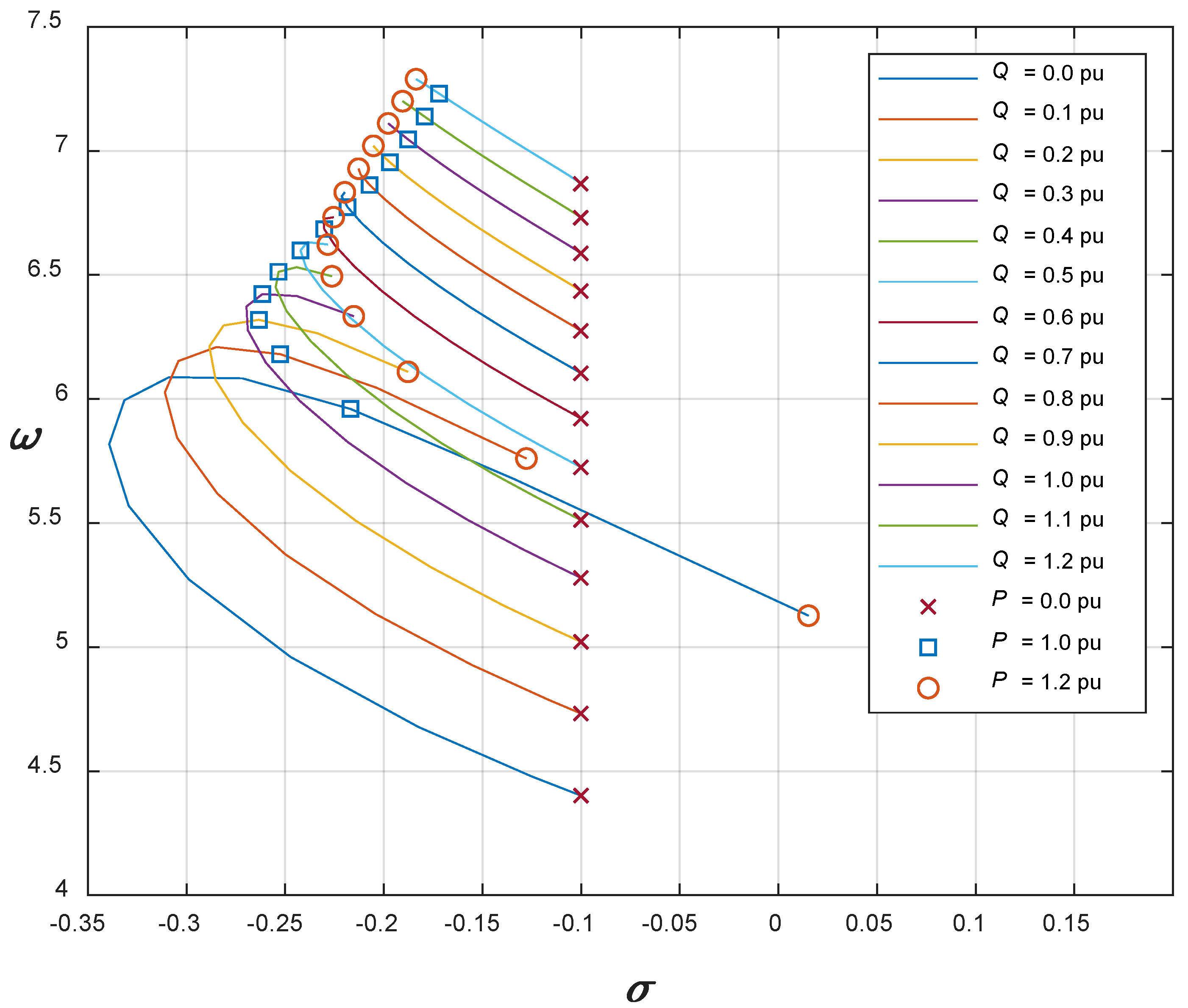
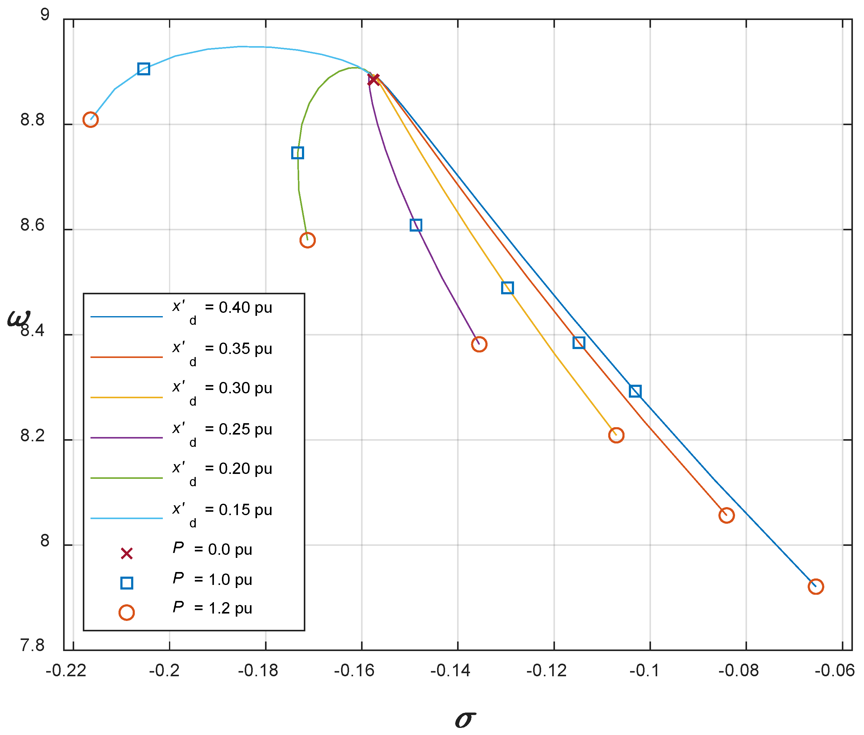
Figure 19.
Eigenvalue loci of local mode of a 158-MVA hydro-type synchronous generator with AVR system at reactive power Q = 0.6 pu, and active power values from P = 0.0 pu to P = 1.2 pu for different values of the direct-axis transient reactance xd’.
Figure 19.
Eigenvalue loci of local mode of a 158-MVA hydro-type synchronous generator with AVR system at reactive power Q = 0.6 pu, and active power values from P = 0.0 pu to P = 1.2 pu for different values of the direct-axis transient reactance xd’.
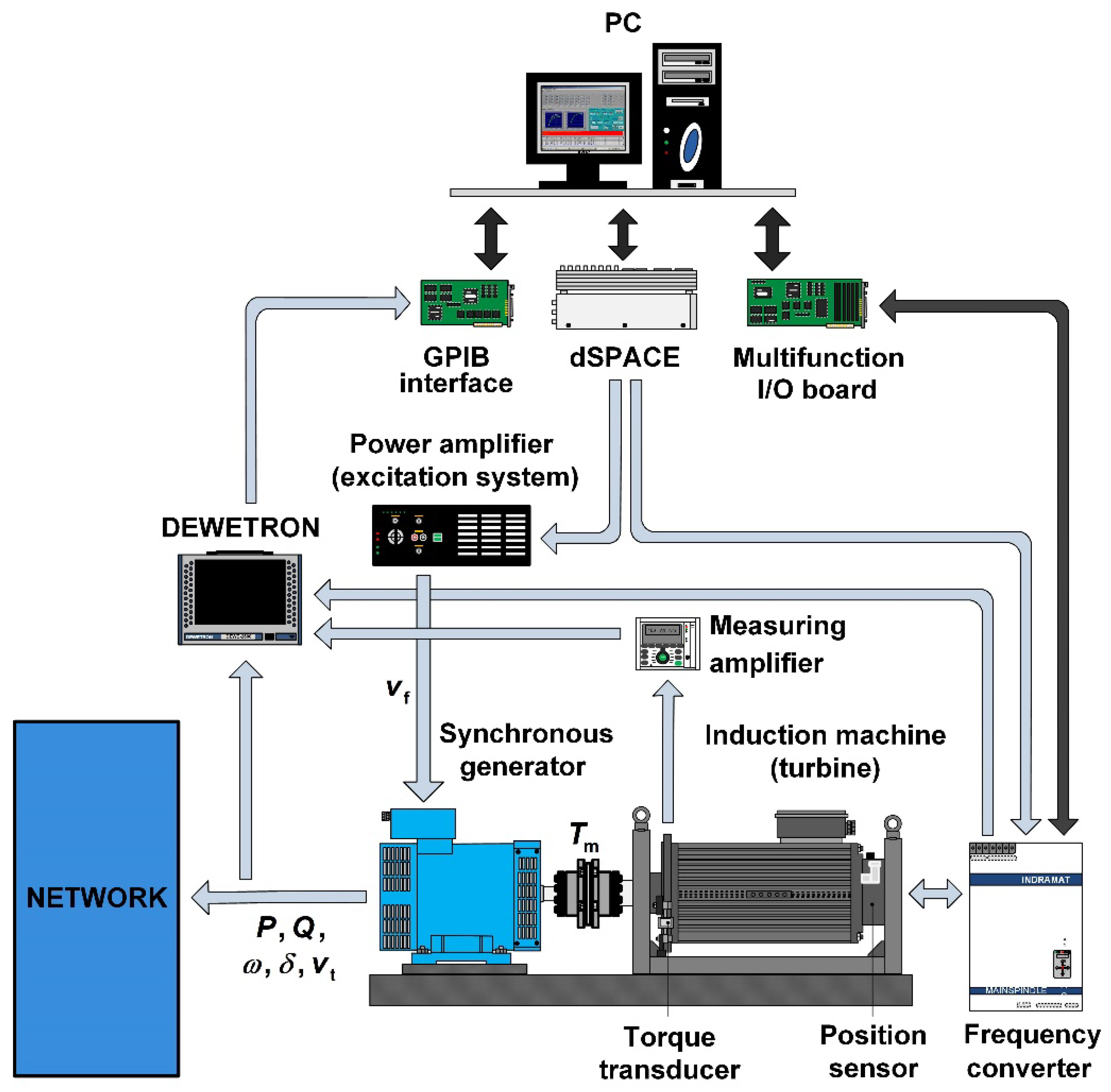
Figure 20.
Laboratory experimental system.
Figure 20.
Laboratory experimental system.
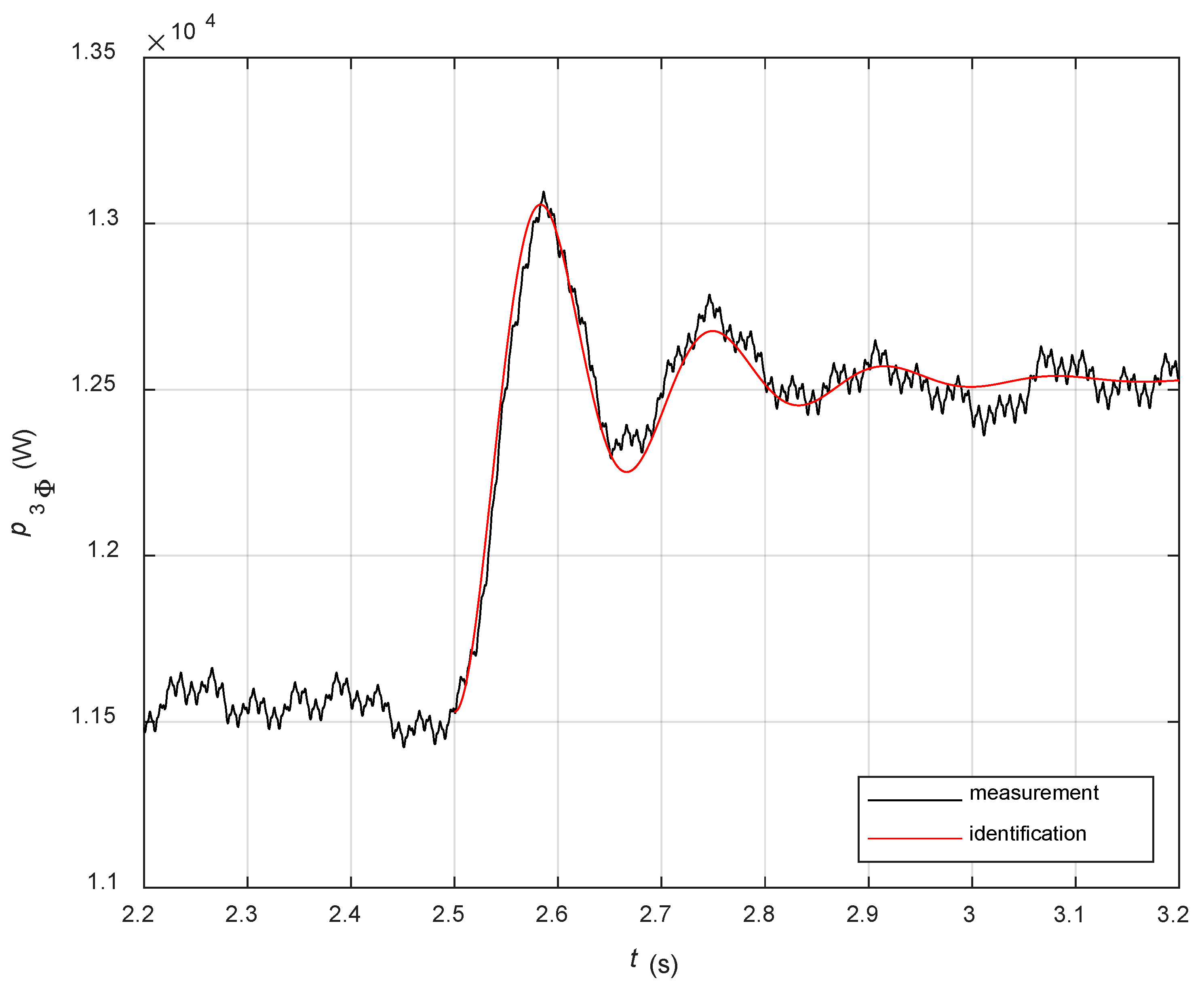
Figure 21.
Time response of the instantaneous three-phase power of the laboratory synchronous generator Sn = 12 kV in the vicinity of the operating point P = 12 kW, Q = 0 kVAr on the step change of mechanical torque corresponding to mechanical power change from 11.5 kW to 13.5 kW compared with the identified local oscillation.
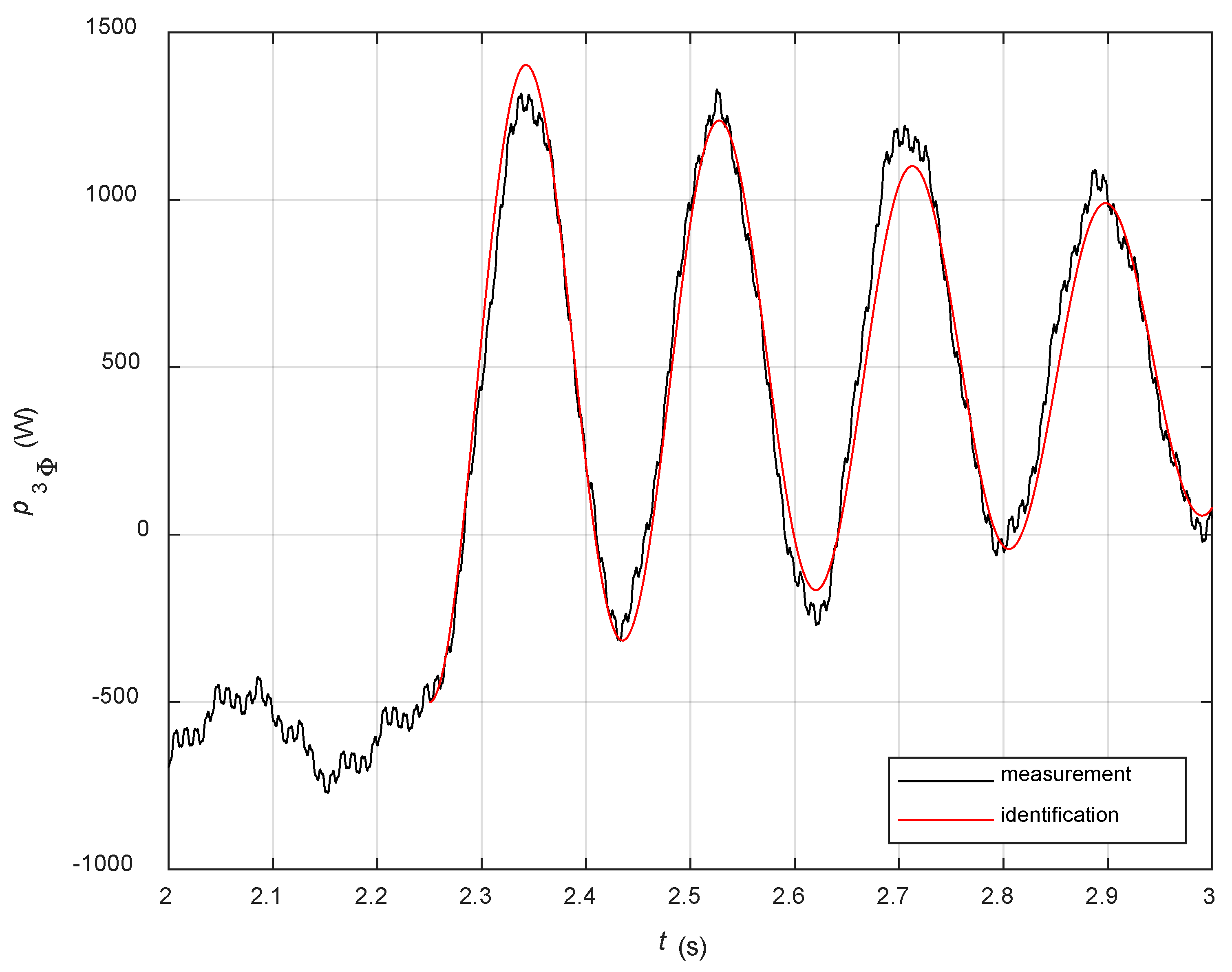
Figure 22.
Time response of the instantaneous three-phase power of the laboratory synchronous generator Sn = 12 kV in the vicinity of the operating point P = 0 kW, Q = 12.0 kVAr on the step change of mechanical torque corresponding to mechanical power change from −0.5 kW to 0.5 kW compared with the identified local oscillation.
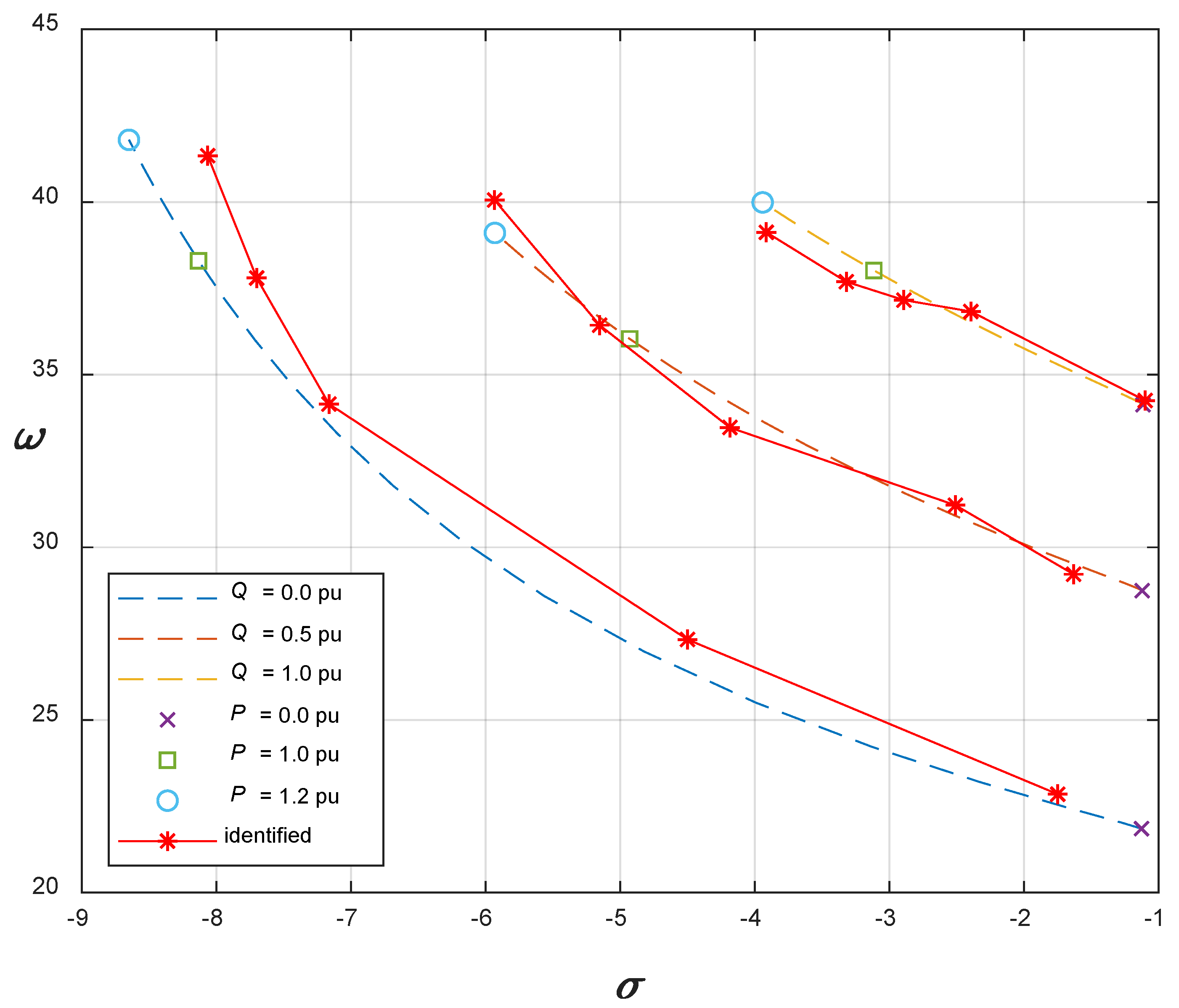
Figure 23.
Eigenvalue loci of the local mode of the laboratory synchronous generator Pn = 12 kW obtained with numerical analysis of an H–P model and with identification of the measured time responses of the oscillations conducted with step changes of the mechanical torque.
Figure 23.
Eigenvalue loci of the local mode of the laboratory synchronous generator Pn = 12 kW obtained with numerical analysis of an H–P model and with identification of the measured time responses of the oscillations conducted with step changes of the mechanical torque.
Table 1.
Data of synchronous generator and network for H–P model parameters calculation.
Table 1.
Data of synchronous generator and network for H–P model parameters calculation.
| Parameters of Synchronous Generator | Ld (H), Lq (H), Ld’ (H), H (s), Re (Ω), Le (H), D (pu), Td0′(s) |
|---|
Operating point
quantities | P (W), Q (Var), ωs (rad s−1), V∞ (V) |
Table 2.
Auxiliary operating point variables necessary for calculation of the parameters of the H–P model.
Table 2.
Auxiliary operating point variables necessary for calculation of the parameters of the H–P model.
Auxiliary operating point
variables | δop, Vd,op, Vq,op, Id,op, Iq,op, Eop, E′q,op, Eqa,op |
Table 3.
The boundaries of real and imaginary parts of local mode eigenvalues of hydro and turbo synchronous generators of different nominal powers in an operating range from P = 0.0 pu to P = 1.2 pu and from Q = 0.0 pu to Q = 1.2 pu.
Table 3.
The boundaries of real and imaginary parts of local mode eigenvalues of hydro and turbo synchronous generators of different nominal powers in an operating range from P = 0.0 pu to P = 1.2 pu and from Q = 0.0 pu to Q = 1.2 pu.
| | Σmin | σmax | ωmin (s−1) | ωmax (s−1) |
|---|
| hydro-generators | −0.4558 | −0.0399 | 2.8554 | 10.8259 |
| turbo-generators | −0.8871 | −0.0807 | 3.6418 | 10.5455 |
Table 4.
The boundaries of real and imaginary parts of local mode eigenvalues of hydro and turbo synchronous generators of different nominal powers in an operating range from P = 0.0 pu to P = 1.0 pu and from Q = 0.0 pu to Q = 1.0 pu.
Table 4.
The boundaries of real and imaginary parts of local mode eigenvalues of hydro and turbo synchronous generators of different nominal powers in an operating range from P = 0.0 pu to P = 1.0 pu and from Q = 0.0 pu to Q = 1.0 pu.
| | σmin | σmax | ωmin (s−1) | ωmax (s−1) |
|---|
| hydro-generators | −0.3193 | −0.0399 | 3.3636 | 9.1832 |
| turbo-generators | −0.6361 | −0.0807 | 3.6418 | 9.4520 |
Table 5.
The boundaries of real and imaginary parts of local mode eigenvalues of hydro and turbo synchronous generators with AVR systems of different nominal powers in the range P = 0.0 pu to P = 1.2 pu and from Q = 0.0 pu to Q = 1.2 pu.
Table 5.
The boundaries of real and imaginary parts of local mode eigenvalues of hydro and turbo synchronous generators with AVR systems of different nominal powers in the range P = 0.0 pu to P = 1.2 pu and from Q = 0.0 pu to Q = 1.2 pu.
| | σmin | σmax | ωmin (s−1) | ωmax (s−1) |
|---|
| hydro-generators | −0.2156 | 0.2804 | 2.9230 | 10.8261 |
| turbo-generators | −0.6421 | 0.3247 | 3.6418 | 10.5310 |
Table 6.
The boundaries of real and imaginary parts of local mode eigenvalues of hydro and turbo synchronous generators with AVR systems of different nominal powers in the range P = 0.0 pu to P = 1.0 pu and from Q = 0.0 pu to Q = 1.0 pu.
Table 6.
The boundaries of real and imaginary parts of local mode eigenvalues of hydro and turbo synchronous generators with AVR systems of different nominal powers in the range P = 0.0 pu to P = 1.0 pu and from Q = 0.0 pu to Q = 1.0 pu.
| | σmin | σmax | ωmin (s−1) | ωmax (s−1) |
|---|
| hydro-generators | −0.2156 | 0.0014 | 3.3636 | 9.1831 |
| turbo-generators | −0.6421 | −0.0809 | 3.6418 | 9.4307 |
Table 7.
Manufacturer’s data of the tested synchronous generator.
Table 7.
Manufacturer’s data of the tested synchronous generator.
| Pn = 12 [kW] | Un = 400 [V] | In = 21.7 [A] | cos φn = 0.8 |
| UFn = 400 [V] | IFn = 21.7 [A] | fn = 50 [Hz] | nn = 1500 [min−1] |
Table 8.
Synchronous generator’s data obtained with tests.
Table 8.
Synchronous generator’s data obtained with tests.
| Ld = 2.11 [pu] | Lq = 1.45 [pu] | Ld′ = 0.25 [pu] | Ld″ = 0.18 [pu] |
| ld = 0.15 [pu] | lq = 0.15 [pu] | Re = 0.003 [pu] | Le = 0.03 [pu] |
| Rs = 0.05 [pu] | RF = 0.015 [pu] | H = 0.19 [pu] | D = 1 [pu] |
| RD = 0.262 [pu] | RQ = 1.08 [pu] | T′d0 = 0.5 [s] | ωs = 2π50 [s−1] |
Table 9.
Linearization parameters of the H–P model for nominal operating point Sn = 15 kVA, cos φn = 0.8.
Table 9.
Linearization parameters of the H–P model for nominal operating point Sn = 15 kVA, cos φn = 0.8.
| Pn = 0.8 [pu] | K1 = 2.1555 | K2 = 2.0815 | K3 = 0.1285 |
| Qn = 0.6 [pu] | K4 = 3.5155 | K5 = 0.0228 | K6 = 0.0998 |
Table 10.
Real and imaginary parts of the eigenvalues, the undamped natural frequencies, and the damping ratios of the local oscillations of the laboratory synchronous generator at different operating points.
Table 10.
Real and imaginary parts of the eigenvalues, the undamped natural frequencies, and the damping ratios of the local oscillations of the laboratory synchronous generator at different operating points.
| | P = 0.0 pu | P = 0.4 pu | P = 0.8 pu | P = 1.0 pu | P = 1.2 pu |
|---|
| Q= 0.0 pu | σ = −1.75 | σ = −4.50 | σ = −7.16 | σ = −7.70 | σ = −8.06 |
| ω = 22.85 | ω = 27.33 | ω = 34.15 | ω = 37.80 | ω = 41.34 |
| ω0 = 22.92 | ω0 = 27.70 | ω0 = 34.89 | ω0 = 38.57 | ω0 = 42.12 |
| ζ = 0.0764 | ζ = 0.1625 | ζ = 0.2053 | ζ = 0.1996 | ζ = 0.1915 |
| Q= 0.5 pu | σ = −1.63 | σ = −2.51 | σ = −4.18 | σ = −5.15 | σ = −5.93 |
| ω = 29.22 | ω = 31.22 | ω = 33.47 | ω = 36.43 | ω = 40.06 |
| ω0 = 29.26 | ω0 = 31.32 | ω0 = 33.73 | ω0 = 36.79 | ω0 = 40.49 |
| ζ = 0.0558 | ζ = 0.0801 | ζ = 0.1241 | ζ = 0.1400 | ζ = 0.1465 |
| Q= 1.0 pu | σ = −1.10 | σ = −2.39 | σ = −2.89 | σ = −3.32 | σ = −3.91 |
| ω = 34.25 | ω = 36.83 | ω = 37.16 | ω = 37.69 | ω = 39.12 |
| ω0 = 34.27 | ω0 = 36.91 | ω0 = 37.27 | ω0 = 37.84 | ω0 = 39.32 |
| ζ = 0.0321 | ζ = 0.0649 | ζ = 0.0776 | ζ = 0.0877 | ζ = 0.0996 |


