Abstract
Past waste disposal practices have left large volumes of sulphidic material stockpiled in a Ramsar wetland site on the Atlantic coast of southwestern Spain, leading to severe land degradation. With the aim of addressing this legacy issue, soil core samples were collected along two transects extending from the abandoned stockpiles to the adjacent marshland and subjected to XRD, SEM-EDS, ICP-OES and ICP-MS analyses. Sulphide oxidation has been shown to be a major driver of acid generation and metal leaching into the environment. The marsh soil receiving acid discharges from the sulphide wastes contains elevated levels (in mg kg−1) of Pb (up to 9838), As (up to 1538), Zn (up to 1486), Cu (up to 705), Sb (up to 225) and Tl (up to 13), which are retained both in relatively insoluble secondary minerals (mainly metal sulphates and oxides) and in easily soluble hydrated salts that serve as a transitory pool of acidity and available metals. By using a number of enrichment calculation methods that relate the metal concentrations in soil and their baseline concentrations and regulatory thresholds, there is enough evidence to conclude that these pollutants may pose an unacceptable risk to human and ecological receptors.
1. Introduction
Acid generation and metal release from oxidative dissolution of sulphide minerals, primarily pyrite, is one of the most serious environmental concerns in many historic mining districts worldwide [1,2]. Contamination arising from acid mine drainage (AMD) not only adversely affects the water quality of downstream waterbodies [3,4,5], but also may cause soil degradation and hazards to human health and the environment around the mine sites [6,7,8,9]. This situation becomes more challenging and harder to manage when ecologically sensitive wetlands appear to be impacted by AMD effects related to improper disposal of hazardous mining waste. The weathering processes may be similar in terms of mineral oxidation and dissolution; however, the hydrologic regime, the rates of reaction, and the environmental consequences can be quite different [10,11,12]. Geochemical reactions and mineral transformations resulting from direct interaction of AMD with coastal wetlands highly vulnerable to contamination are not yet fully understood and require further research to address their environmental implications.
The estuary of Huelva, on the southwestern Spanish coast, provides the opportunity to assess land degradation processes driven by weathering of abandoned sulphide-rich wastes in a coastal wetland. Past mineral-processing operations have left a legacy of large amounts of pyrite concentrates stockpiled on the banks of the salt marsh (Figure 1). The ores extracted from the Tharsis and La Zarza mines in the Iberian Pyrite Belt (IPB) were transported by railway to the estuary to be shipped overseas. Prior to shipment, the ore was crushed, ground, and screened in processing plants located at the railway terminal of Corrales near the loading dock, facing the city of Huelva (Figure 2). The last mining operation closed at the end of December 2000 for economic reasons. Consequently, the pyrite concentrates stored in piles at the processing facilities were left without any remediation plan to mitigate the environmental impacts of the abandoned stockpiles on the adjacent wetland ecosystem. During the operational phase, and especially since the closure of the ore processing activity, the pollutants have been and still are being transferred from the sulphide heaps to nearby marsh soils, resulting in the deterioration of environmental quality [13]. It is particularly concerning that a considerable portion of the wasteland was converted for urban development.
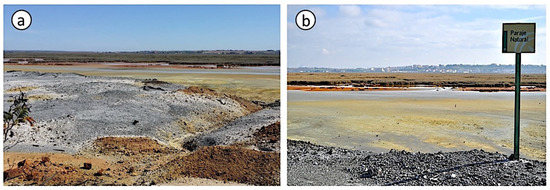
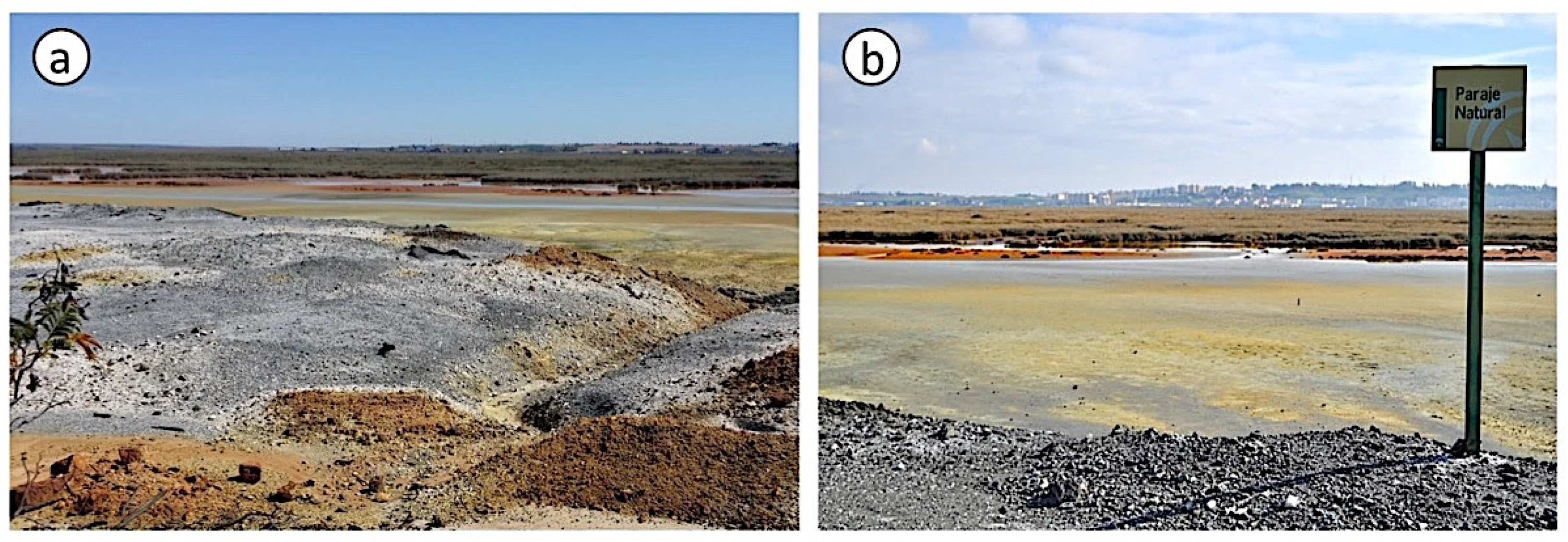
Figure 1.
Field pictures of the degraded land area showing the abandoned stockpiles of crushed pyrite ore (a) and the salt marsh soil affected by the acid drainage (b).
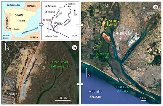
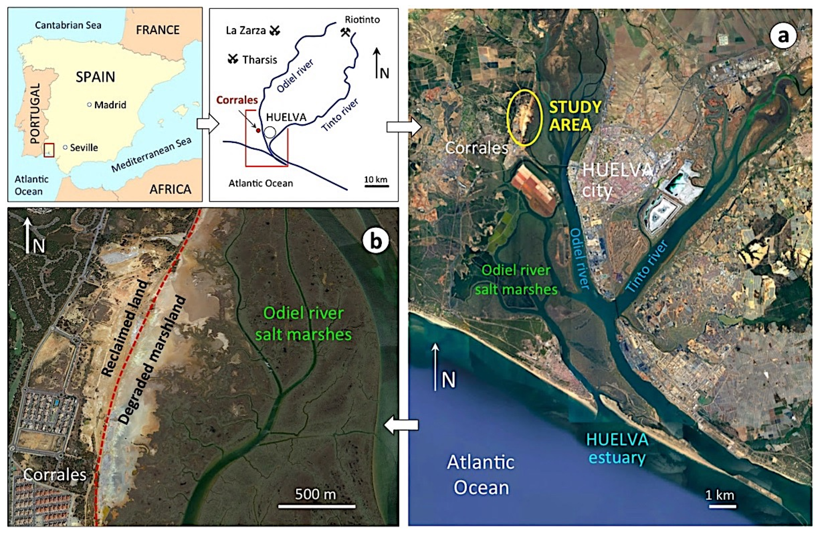
Figure 2.
Geographical setting of the Huelva estuary showing the location of the study area (a) and the salt marsh soil impacted by past mineral handling activities (b).
From the entry into force of the contaminated land regime in Spain [14], the parcels that had been re-classified for residential use were declared as polluted in 2007 because the site posed unacceptable risks to human health by exposure to potentially toxic trace elements (PTEs). In 2009, the sulphide wastes were removed from the private parcels and the underlying soil was lime-treated to neutralize acidity and sealed with compacted clay to prevent seepage and the release of pollutants. However, the stockpiles within the maritime–terrestrial public domain, occupying an area of about 15,000 m2, still remain unreclaimed and continue to pose a risk to human health and the environment [15].
Knowledge of the geochemical and mineralogical variability and the extent or degree of contamination is crucial in developing the remediation strategies that are currently being considered by the regional authorities, because AMD minerals usually carry varying amounts of PTEs and are responsible for the production of acid upon dissolution [16]. The aims of this paper are therefore to (1) determine the spatial distribution (laterally and vertically) of PTEs in the marsh soil acidified by AMD; (2) infer the chemical weathering reactions occurring in the sulphide heaps and the mineral transformations driven by acid generation and metal release; (3) ascertain the mineralogical controls on dispersal, storage and remobilization of PTEs; and (4) evaluate the contamination status of the site and the potential threats to human and ecosystem health.
2. Study Area
The former industrial site of Corrales lies on the west side of the upper estuary of Huelva, directly across from the salt marshes of the river Odiel (Figure 2). These marshes form part of a set of coastal wetlands with high ecological value, declared in 1983 to be a UNESCO Biosphere Reserve. The area is characterized by a Mediterranean climate moderated by the influence of the Atlantic Ocean, with mild, relatively rainy winters and hot, sunny summers. The average annual precipitation is 525 mm, and the mean temperature ranges from 11.0 °C (January) to 25.8 °C (July–August).
The estuarine marsh soils are Salic Fluvisols (soil classification according to World Reference Base for Soil Resources [17]) developed on fluvio-marine silty-clayey sediments. The soil profile is AC or ABC type, with a salic horizon within 50 cm from the surface and hydromorphic features in the lower horizons. In dry periods, the soil usually contains salt efflorescence at the surface, forming a coating layer. The wetland vegetation is dominated by salt-tolerant plant species [18], except in the vicinity of the sulphide waste piles where the salt marsh is entirely devoid of vegetation.
The marshland directly affected by AMD discharges has a surface area of about 50 ha, and shows a well-defined chromatic zonation. The abandoned sulphide stockpiles have a distinct grayish colour (Hue GLEY 1 in the Munsell colour chart). The yellow zone (2.5Y to 5Y) contains abundant secondary products of pyrite oxidation and yellow efflorescent sulphate salts. The soil of the white zone (10YR to 2.5Y) has more frequent interaction with the tidal dynamics and exhibits efflorescent salt deposits. The surface soil of the most distal zone is reddish-ochre in colour (5YR to 7.5YR), which denotes a high degree of oxidation of iron. The floodplain is excavated by tidal channels filled with fine-grained yellowish sediment (2.5Y to 5Y).
3. Materials and Methods
3.1. Sampling and Sample Preparation
To reduce selection bias and collect representative samples of the degraded marsh, the sampling area was subdivided into three tidal flat zones based on the dominant colour of the surface soil, namely the yellow zone, white zone, and ochre zone, which are aligned in a north–south direction nearly parallel to the sulphide stockpiles that lie directly on the soil adjacent to the marshland (Figure 3). The samples chosen are representative of the Salic Fluvisol adversely affected by continuous discharges of AMD.
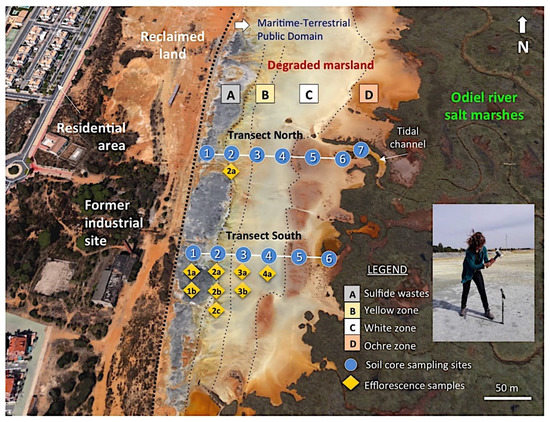
Figure 3.
Aerial view (Google Earth) of the degraded wetland showing the location of the soil cores collected along two linear transects spanning from the abandoned sulphide heaps to the salt marshes. Figure inset shows the soil core sampling method.
Forty samples were collected in cores along two linear transects of approximately 150 m in length spaced 120 m apart (Supplementary Figure S1), including the sulphide waste samples. Line transects were positioned perpendicular to the riverbank and randomly set up across the degraded marshland. Six undisturbed cores were taken at about 25 m intervals along each transect. The cores were extracted using a gouge auger (100 cm length and 30 mm diameter) with hammer, then divided transversely into several sections representative of different depth intervals within the soil profile based on field observations of soil colour and texture. An additional soil core was augered in the tidal channel near location 6 of the northern transect.
The soil samples were air-dried, gently disaggregated with a wooden roller, passed through a 10-mesh nylon sieve and blended to achieve a high degree of homogeneity. After homogenization, aliquots of sieved material (<2 mm) were ground in an agate mortar and pestle until a nearly uniform fine powder (<63 μm) was obtained for mineralogical and chemical analysis.
Additionally, in dry-weather conditions, eight efflorescent salts were collected with a stainless-steel spatula, placed in tightly sealed plastic containers to prevent dehydration, and immediately transported to the laboratory for analysis.
3.2. Analytical Methods
Soil active reaction (pHH2O) was potentiometrically determined in a soil to deionized water suspension of 1:2.5 (w/v) after shaking for 15 min followed by a 30 min equilibration period. Potential acidity (pHKCl) was determined by measuring soil pH in a 1.0 M KCl solution using the same protocol. The difference between pH(H2O) and pH(KCl) values gives a measurement of exchangeable acidity.
Mineralogical analysis was performed by X-ray diffraction (XRD) on a Bruker AXS D8-Advance diffractometer using CuKα radiation at 40 kV and 30 mA. Randomly oriented powders were scanned with a step size of 0.02° and a counting time of 0.6 s per step. The XRD patterns were processed using DIFFRAC plus software linked with a reference database, and relative mineral abundance was estimated by empirical intensity factors weighting the integrated peak areas of diagnostic reflections [19].
Selected soil samples and all the efflorescent salt samples were examined by environmental scanning electron microscopy (ESEM) using a FEI-Quanta 200 instrument operated at 20 kV and equipped with an energy-dispersive spectrometer (EDS), combining back-scattered electron (BSE) imaging with EDS microanalysis to assist in the mineral identification.
Total concentrations of major and trace elements were analysed by inductively coupled plasma optical spectroscopy (Agilent 5110 ICP-OES) and inductively coupled plasma mass spectrometry (Agilent 7900 ICP-MS), respectively, following multi-acid digestion (HClO4-HNO3-HCl-HF). Analytical quality control was monitored by the use of international certified reference materials (AGW-1 and SARM-4), blanks and duplicates to check the accuracy and precision of the data. The relative standard deviations of the analyses were typically below 5% for major elements and better than 10% for trace elements.
3.3. Data Analysis
A statistical evaluation of the analytical data including descriptive statistics and univariate and multivariate correlation analysis was performed using the STATISTICA 10.0 software package. The strength of the linear relationship between total concentrations of PTEs was quantified by the coefficient of determination (R2), and the influence of the interrelated variables was accomplished by principal component analysis (PCA). A normalized Varimax rotation was applied to the axes of the principal components in order to maximize the variance of the factors.
The soil contamination status was assessed by a number of enrichment calculation methods that relate the concentrations of PTEs in soil and their baseline concentrations [20,21,22]. To quantify the enrichment factor of each PTE [23], the measured concentration was normalized against the content of a conservative lithogenic trace element, as follows:
where EF is the enrichment factor, Cx is the concentration of the element of concern and Cref is the concentration of the reference element. In this study, zirconium (Zr) was chosen as the reference element for normalization.
The pollution load index (PLI) was used to calculate the degree of multielement soil contamination by deriving the nth root of the n factors [24]:
where CF is the contamination factor, i.e., the quotient between the PTE concentration in the sample and its background concentration [25], and n is the number of PTEs evaluated. PLI values above one would indicate progressive deterioration of estuarine marsh soil quality.
The geoaccumulation index (Igeo) is another numerical indicator used to evaluate the contamination levels for the recovered soil cores, as follows [26]:
where Cn is the measured concentration of PTE in the sample, Bn is its background value, and 1.5 is a matrix correction factor due to lithogenic effects.
Finally, the potential ecological risk index (ERI) of multi-metal(loid)s [25] was calculated using the contamination factors of the most relevant PTEs (As, Cd, Cu, Pb, and Zn) occurring in the topsoil:
where n is the number of elements involved (in this case, n = 5), Eri is the potential ecological factor for the given element (i), Tri is the toxic-response factor for the given element, and Ci is the contamination factor for the given element.
4. Results
4.1. Sulphide Wastes
The abandoned waste piles are composed essentially of fine-grained pyrite, and also contain quartz pebbles and a variety of artifacts and materials of anthropic origin, such as fragments of bricks, glass, wood, pottery, etc. The samples from these pyritic residues showed ultra-acid pH(H2O) values (Table 1) ranging from 1.10–1.25 (top core samples) to 1.60–1.73 (bottom samples), with an average of 1.3–1.5. The pH(KCl) values were somewhat lower, averaging 1.2–1.3; hence, active and potential soil reaction are nearly similar. The soil underlying the wastes was found to be severely acidified, with pH(H2O) values being 2.5 at the depth of 50–70 cm.

Table 1.
Soil pH values in water (actual acidity) and in KCl (potential acidity), and mineral composition of the soil core samples and efflorescent crusts. Mineral abbreviations as defined in Supplementary Table S1.
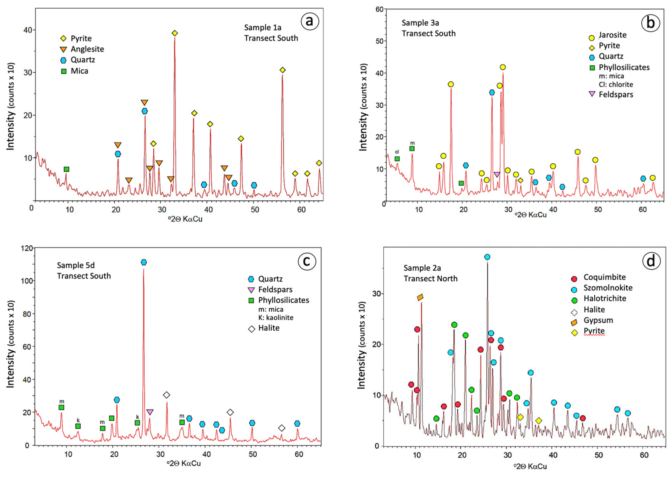
The results from the XRD analysis confirmed that pyrite is the dominant sulphide phase (Figure 4a), and SEM-EDS examination revealed the occurrence of epitaxial overgrowths of anglesite on barite (Figure 5a). The soil on which the sulphide wastes were stockpiled is composed mainly of quartz, mica and kaolinite, with minor feldspars and some pyrite transferred downward from the heaps.
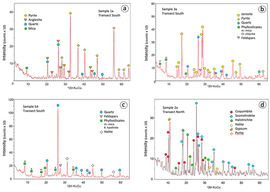
Figure 4.
Powder XRD diffractograms of representative samples of the sulphide wasteland (a), yellow zone (b), ochre zone (c), and sulphate crusts (d).
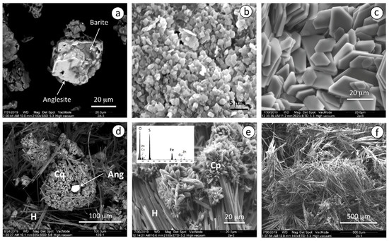
Figure 5.
SEM images showing: (a) epitaxial overgrowth of anglesite on barite; (b) micron-sized crystals of jarosite; (c) tabular crystals of copiapite with pseudo-orthorhombic symmetry; (d) efflorescent mixture of coquimbite (Cq) and halotrichite (H) with anglesite (Ang); (e) inset EDS spectrum of copiapite (Cp) grown on fibrous aggregates of halotrichite (H); and (f) bundled, fibrous crystals of halotrichite.
As expected, the sulphidic waste material is chemically characterized by elevated concentrations of iron and sulphur (Table 2 and Table 3). The maximum contents of Al2O3 (14.48%) and K2O (2.01%) were measured in the deepest sample, where the mineralogical influence of the substrate becomes more apparent. The sulphide wastes have extremely high levels of PTEs (in mg kg−1), particularly Pb (up to 34,754) and Zn (3665), as well as Cu (810) and some metalloids, As (828) and Sb (1563). The concentrations of Se (26.3), Tl (16.4) and Cd (10) found in some samples are also relevant.
Table 2.
Chemical composition of major and trace elements of the soil core samples collected along the north transect.
Table 3.
Chemical composition of major and trace elements of the soil core samples collected along the south transect.
4.2. Surface and Subsurface Soils
Soil active acidity varied greatly along the sampling sites, and even within the soil profile (Table 1). The lowest pH(H2O) values (1.68–1.84) were registered in the yellow zone adjacent to the sulphide piles. Soil core 6 (transect north) of the ochre zone showed a remarkable increase in pH(H2O) with depth, changing from 3.63 to 6.29 within 30 cm. In the ochre zone the pH(KCl) was by about 0.6 units lower than the pH(H2O), which is indicative of some salt-replaceable acidity. Another potential pool of soil acidity arises from the eventual oxidation of pyrite.
Pyrite occurs in most soil core samples of the yellow and white zones. It is relatively abundant in the topsoil of the yellow zone and in certain samples from the subsurface levels. In the ochre zone, pyrite is also present as a minor component. Under SEM examination, the crystals of pyrite usually exhibit dissolution pits on surfaces.
Jarosite was found in soil samples with pH values ranging between 1.6 and 4.3. It is the most abundant and widespread of the AMD minerals in the soil around the waste disposal area, and responsible for the distinctive yellow colour of this proximal zone. The tidal channels are filled with jarosite-rich (over 70%) mud. Jarosite also occurs as a subordinate mineral in the white zone, whereas it is lacking in the ochre one. In most samples, the XRD pattern (Figure 4b) fits well with the standard pattern of natrojarosite, which is another jarosite-group mineral with Na instead of K. The SEM-EDS analysis confirmed that they were indeed composed of up to 7% Na2O. Fine aggregates of natrojarosite seen under SEM exhibit pseudocubic crystals less than 1 μm in size (Figure 5b).
Quartz, mica, kaolinite, and feldspars were found in all samples in varying amounts. These silicates are dominant in the deeper core samples of the distal zones (Figure 4c), as they are primary components of the native soil. In addition, a variety of resistant accessory minerals such as amphibole, barite, monazite, and zircon were detected by SEM-EDS. Iron oxides, notably hematite, occur mainly in the most distal zone, giving rise to the reddish-ochre colour of the soil. Halite is present in the sampling sites closest to the salt marsh, that is, in the white and ochre zones, where the tidal influence is strongest.
Major and trace element concentrations in soil samples are listed in Table 2 and Table 3. The soil geochemistry is largely dominated by iron (up to 51.76% Fe2O3) and sulphur (up to 49.03% S), which is compatible with the mineral composition of the acid sulphate soils. There is a good positive correlation between Fe2O3 and total sulphur (R2 = 0.73) because of the presence of pyrite and/or jarosite in many samples, except in the soils of the ochre zone where Fe is mainly in the form of oxides. Alumina is a major constituent of the soil samples from the distal zone (up to 19.11% Al2O3), reflecting the abundance of clay minerals (mica and kaolinite); hence Al2O3 appears strongly inversely correlated with Fe2O3 (R2 = −0.83). All of the other major elements appear in lower concentrations. The highest K2O content (5.74–6.48%) is observed in the tidal channel, where jarosite is the dominant phase. In the ochre zone, K2O is well correlated (R2 = 0.78) with Al2O3 due to the occurrence of dioctahedral mica. The relatively high content of Na (up to 4.53% Na2O) found in the yellow zone is linked to natrojarosite, whereas in the white and ochre zones (up to 3.45% Na2O) it is mostly related to halite. While Mg is more abundant in the ochre zone (up to 2.16% MgO), Ca is present in all samples at concentrations less than 1% CaO, its distribution being controlled largely by gypsum.
In the transect south (Table 2), the highest concentrations of PTEs were measured in the surface soil adjacent to the sulphide heaps, reaching values (in mg kg−1) up to 9838 Pb, 1538 As, 1486 Zn, 705 Cu, 225 Sb, 83 Co, 13 Tl, and 4.6 Cd. The concentrations decreased toward the marshes, with values (in mg kg−1) as low as 79 Pb, 37 As, 139 Zn, 90 Cu, 3.8 Sb, 0.71 Tl, and 0.33 Cd. The distribution pattern in the northern transect (Table 3) is similar to that of the southern transect. The upper part of the soil adjoining the sulphide piles contains the highest concentrations (in mg kg−1) of Pb (9174), Zn (676), Sb (457), Co (189), Sn (44.7), Tl (19.2), Se (8.8), and Cd (2.29), whereas the most extreme values of As (4223) and Cu (1958) were measured in the jarosite-rich tidal channel infills. As noted in the south transect, the concentrations of all these PTEs decreased from the source of sulphide oxidation toward the salt marsh.
4.3. Efflorescent Minerals
In periods of dryness, as surface soil dries out the exposed surfaces of the sulphide piles and the area of the marsh degraded by the effects of acidification and metal contamination are covered with multicoloured efflorescences of readily water-soluble sulphate salts (Figure 6). The efflorescent blooms are temporary because of the high solubility of these salts [27] and their susceptibility to dissolution by rain or high tide flooding.

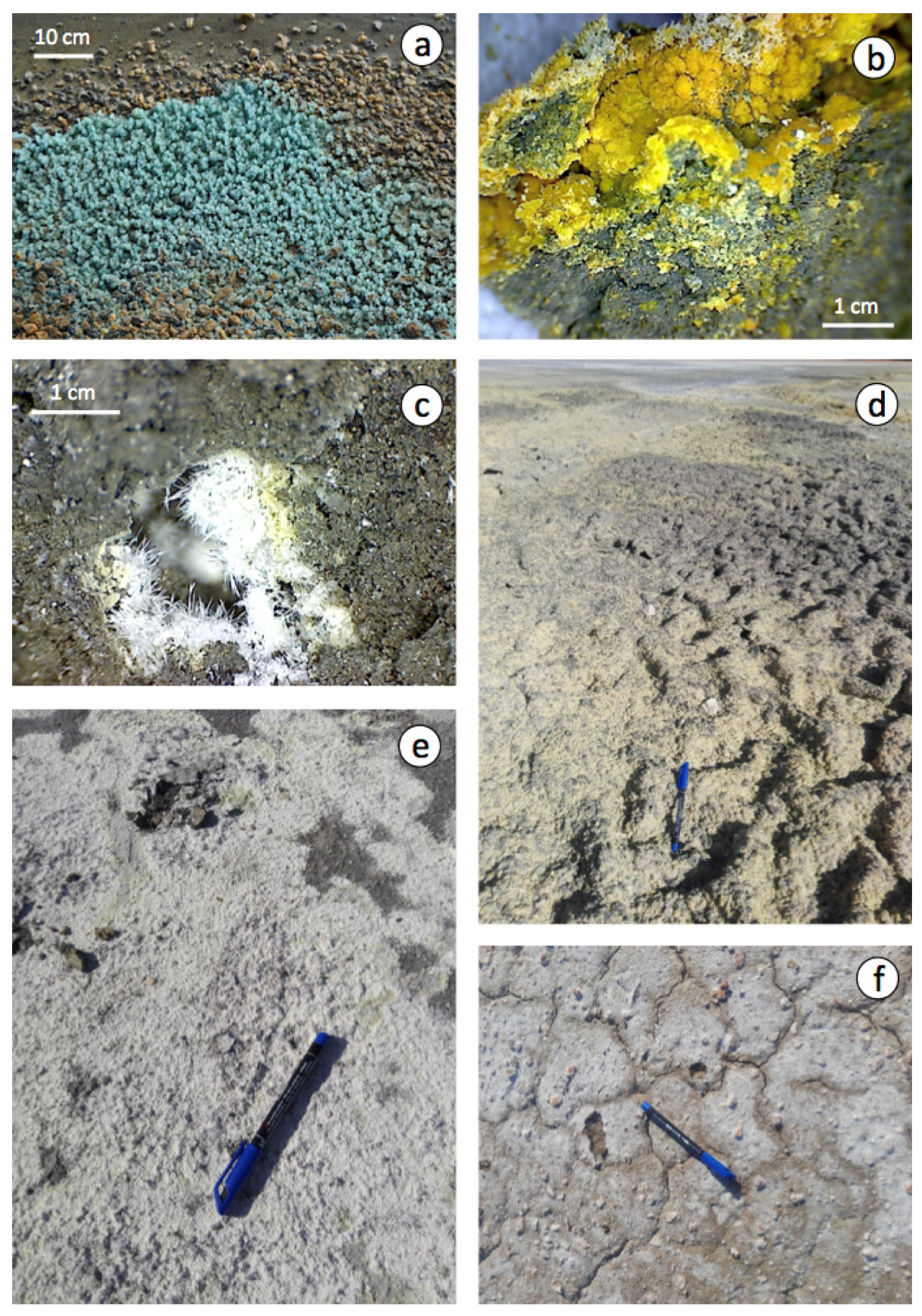
Figure 6.
Efflorescent blooms of sulphate minerals on the surface of the pyrite wastes: (a) greenish-blue crystals of melanterite; (b) fine-grained yellow crust of copiapite; (c) white hairy halotrichite; (d,e) yellow to white encrustations of mixtures of soluble sulphate salts covering the floodplain; and (f) crystallization of efflorescent halite on soil surface with desiccation cracks (distal zone).
A variety of evaporitic sulphate minerals with different hydration degrees was identified by combining XRD and SEM-EDS analyses (Table 1). Melanterite typically forms greenish-blue crust-like aggregates on pyrite, and the other Fe–sulphate minerals generally occur as encrustations or efflorescent mixtures, with copiapite, coquimbite, szomolnokite and halotrichite being the most common precipitates associated with sulphide oxidation (Figure 5c–f). Although the secondary sulphate minerals are typically Fe-dominant, Mg-dominant sulphates (epsomite and hexahydrite) and Al-bearing sulphates (halotrichite and alunogen) form abundantly as well. The efflorescent sulphate salts provide an important source of acidity (1–2 pHH2O units) upon dissolution.
Overall, the geochemistry of the major elements is consistent with the chemical composition of the mineral assemblages determined by XRD (Figure 4d), with iron and sulphur being the prevalent elements. The efflorescent samples differ mainly in their content of Na, K, Ca, and Al due to the occurrence of halite, jarosite, gypsum, and halotrichite, respectively. Regarding total concentrations of PTEs, the sulphate crusts are characterized by relative high contents of Cu, Zn and As. EDS microanalysis of selected crystals has detected appreciable amounts of Cu (2–3% CuO) and (6.6–8.6% ZnO) replacing Fe in the crystal lattice of copiapite.
5. Discussion
5.1. Acid Generation and Release
The sulphide wastes left in place are an important point source of ultra-acidic waters and dissolved PTEs. In this drainage system, the acid-producing process is driven by the oxidative dissolution of pyrite upon exposure to air and water through a complex series of chemical and bacterially-mediated reactions [10,28,29]:
FeS2 + 7/2O2 + H2O → Fe2+ + 2SO42− + 2H+
Fe2+ + 1/4O2 + H+ → Fe3+ + 1/2H2O
FeS2 + 14Fe3+ + 8H2O → 15Fe2+ + 2SO42− + 16H+
The large surface area of the crushed ore induces high rates of acid production that exceed the acid neutralization capacity of the soil minerals, thus declining the pH to ultra-acid values and enhancing the mobilization of PTEs. The pH of the leachates emanating from the sulphide heaps is in the range of 1.66–2.16 [30]. Accordingly, soil acidity is controlled by the amount of hydrogen ions derived from pyrite oxidation and subsequent Fe3+ hydrolysis. Exchangeable acidity is negligible in the waste environment due to the lack or scarcity of constituents with cation exchange capacity, such as clay minerals and organic matter. The potentially available pool of acid cations on the exchangeable sites of the reactive soil particles tends to increase with distance from the source of sulphide oxidation due to the progressive development of cation exchange reactions. This explains why the difference between the pH(H2O) and pH(KCl) values becomes more pronounced in the soil cores recovered in the distal zone.
In addition to hydrogen ions, high solute concentrations of Fe, sulphate, and PTEs are released into nearby surface waters and soil. Oxidative dissolution of minor base-metal sulphides present in the pyrite ore, such as chalcopyrite, sphalerite and galena, usually does not produce acid; however, if Fe3+ is the oxidant acid is formed through the reactions [31,32]:
CuFeS2 + 16Fe3+ + 8H2O → Cu2+ + 2SO42− + 17Fe2+ + 16H+
PbS + 8Fe3+ + 4H2O → Pb2+ + SO42− + 8Fe2+ + 8H+
ZnS + 8Fe3+ + 4H2O → Zn2+ + SO42− + 8Fe2+ + 8H+
In addition to Cu, Pb and Zn, environmentally hazardous concentrations of As, Cd, Sb, Co, Se, and Tl occurring as isomorphic substitutions in the sulphide lattices are mobilized, thus increasing the amount of PTEs available in the environment. Although water quality data are insufficient to make a reliable determination of metal fluxes in the area, Dávila et al. [30] have estimated the average concentrations of Cu, Zn and As to be 325.7, 185.0 and 34.9 mg L−1, respectively, which is comparable to values emerging from the adits, heap leach piles, waste rock dumps, and tailings of the IPB mine sites [33].
As another result of soil acidification, dissolution of carbonates and hydrolysis of silicates susceptible to chemical weathering provide a reservoir of cations (K+, Na+, Ca2+, Mg2+ and Al3+), which when combined with SO42− and Fe2+ ions lead to the formation of a variety of secondary sulphate minerals. The interaction of estuarine water with soil also contributes to the supply of seawater cations, especially Na+.
5.2. Formation and Evolution of Secundary Minerals
The soil mineralogy of the marshland impacted by AMD is consistent with a depleted carbonate buffering system, in which jarosite and hematite are the most stable phases under the prevailing geochemical conditions. The sulfurization process provides an acidic and oxidizing environment suitable for jarosite (or natrojarosite) formation, at pH less than 3.1 and ~5000 mg L−1 of dissolved sulphate concentration according to Hammarstrom et al. [34] through the reaction:
K+ (Na+) + 3Fe3+ + 2SO42− + 6H2O → K (Na) Fe33+ (SO4)2 (OH)6 + 6H+
Jarosite-group minerals can scavenge and act as sinks for PTEs in AMD-impacted areas [35]. The high contents of As, Sb, and Tl linked to jarosite-rich soil horizons suggest that these contaminants were sequestered by jarosite through structural incorporation or surface adsorption [36], thus enhancing the natural attenuation processes.
Gypsum is another sulphate relatively widespread as a newly-formed mineral, although its relative abundance in the soil is rather low. Its origin is conditioned by the prior dissolution of carbonates that provides the Ca2+ ions necessary to combine with the sulphate ions released into solution by sulphide oxidation, according to the reactions:
CaCO3 + 2H+ → Ca2+ + H2O + CO2
Ca2+ + SO42− + 2H2O → CaSO4·2H2O
The evolution from Fe-sulphate minerals to Fe oxyhydroxides occurs by a combination of dehydration, oxidation and neutralization reactions [16]. As the concentration of dissolved Fe3+ decreases with increasing pH, Fe3+ solubility is limited by the precipitation of ferric oxyhydroxides, such as goethite:
Fe3+ + 2H2O → FeOOH + 3H+
Other poorly-crystallized secondary products such as ferrihydrite and schwertmannite might have previously formed, depending on the geochemical conditions of the AMD system [37,38]; however, these precursors are thermodynamically metastable with respect to goethite [39]. Accordingly, goethite might have formed both by direct precipitation and by transformation of the metastable phases, and over time converted to hematite, which is the dominant Fe phase in the furthest reddish-ochre zone:
2FeOOH → Fe2O3 + H2O
Most of the Pb released by dissolution of galena (Equation (9)) has precipitated at low pH in the form of anglesite, and has thereby been immobilized at or near the source of contamination:
Pb2+ + SO42− → PbSO4
Our SEM observations revealed that anglesite has grown epitaxially on the surface of pre-existing barite crystals, with the latter acting as substrate for heterogeneous nucleation. The removal of Pb2+ ions from the aqueous solution and its persistent storage in anglesite seems to be an effective mechanism of natural attenuation.
During prolonged dry weather, efflorescent blooms of hydrated sulphate salts are formed as products of evaporation of the acidic sulphate-rich solutions derived from oxidizing pyrite. Although the neoformed sulphate minerals are ephemeral, they provide important clues about the precipitation reactions from which they arise and the subsequent mineral transformations occurring with increasing temperature and/or decreasing water activity [27,34,40]. The reactions that lead to secondary sulphate-mineral formation in the study area are schematized in Figure 7.
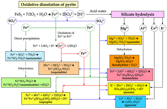
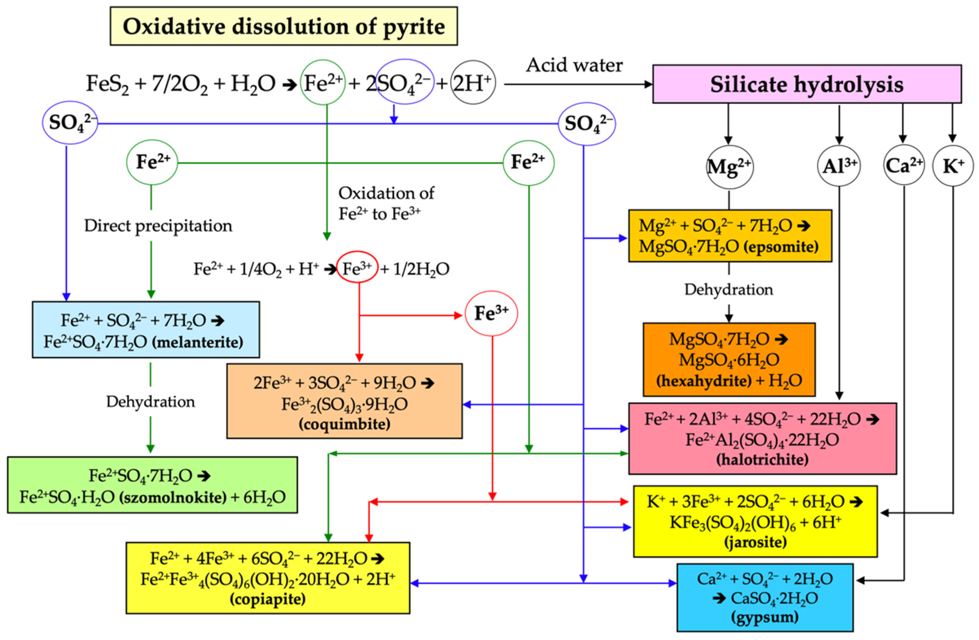
Figure 7.
General flow chart of the chemical reactions involved in the formation of the secondary sulphate minerals.
Melanterite was the first ferrous sulphate to precipitate from the Fe(II)-rich evaporating AMD solution draining directly from the pyrite stockpiles, and was subsequently converted by dehydration into szomolnokite. After oxidation of Fe(II) to Fe(III), copiapite and coquimbite were formed by direct precipitation from the AMD. The combination of sulphate ions with the cations released by silicate hydrolysis led to the formation of halotrichite, alunogen, and epsomite, which becomes hexahydrite by dehydration. These parageneses of soluble sulphate salts and their evolution with time are consistent to those reported in mine sites and AMD-impacted rivers [41,42].
The precipitating efflorescent sulphates incorporate and remove PTEs from the solution, mainly Cu and Zn, and therefore provide a transient storage mechanism for these easily mobile metals. Of particular concern is that the acidic metal–sulphate salts are flushed into receiving estuarine waters during rainfall and high-tide flooding events, causing dramatic pH declines and suddenly increasing the load of sulphates and dissolved metals available to plants in the wetland ecosystem.
5.3. Soil Contamination Assessment
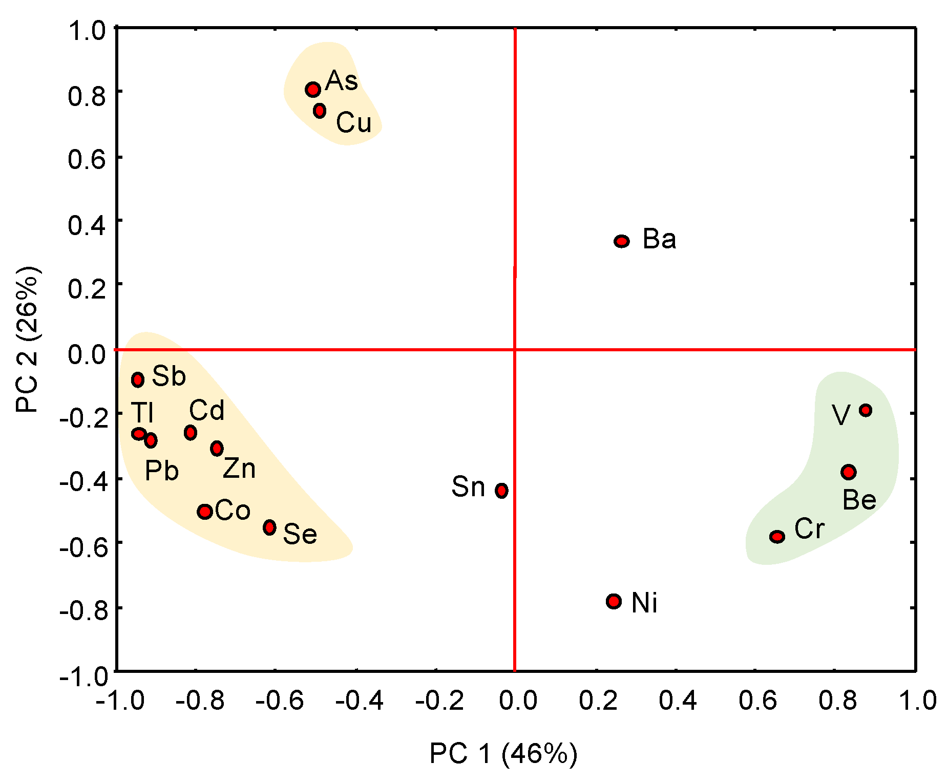
Multivariate statistical analysis showed a clear distinction between naturally occurring trace elements and PTEs transferred from the sulphidic waste piles to the adjacent marshland by both chemical and physical processes (leaching, runoff, atmospheric deposition of wind-blown dust). Several clusters are apparent on the projection of the scores on the first two principal components extracted from the PCA (Figure 8), which account for 72% of the total variance. The first principal component (PC1) is statistically dominant, showing two distinctive clusters characterized by strong and opposite scores: (1) As-Cu-Pb-Zn-Cd-Co-Tl-Sb-Se, and (2) Be-Cr-V. These geochemical associations are interpreted as formed by anthropogenic and geogenic trace elements, respectively, while Ni, Ba and Sn are probably derived from mixed sources.

Figure 8.
PCA diagram of the total concentration of trace elements. Several clusters are apparent on the projection of the scores on the first two principal components (PC1 and PC2), which explain 72% of total variance.
By far the most abundant of the PTEs present in the sulphide waste piles are As, Pb, Cu, Zn and Sb. Consistently, the total concentrations of such elements in most soil core samples are above the median value reported for topsoil of the salt marshes of the Huelva estuary [43] and greatly exceed the regional baseline concentrations [44]. However, a site-specific assessment of soil contamination requires knowledge of pre-industrial metal concentrations to act as a local background against which measured values can be compared [20,45]. In this study, the concentrations of PTEs measured in the least impacted level of soil (core sample 5d, transect south) served as a suitable background or baseline reference material, under the assumption that at this depth (45–60 cm) the cored soil would not be contaminated by anthropogenic inputs.
The EF appears to be an effective indicator to reveal the anthropogenic source of the PTEs of concern. The results from the EF calculation (Table 4) suggest extremely high enrichment levels of Pb (up to 1893) and Sb (1578) as well as Tl (494), As (380), Cd (225), Zn (158), and Cu (106) in the soil of the yellow zone. It is also noteworthy that the tidal channel infill showed high EF values for As (369) and Sb (133). By contrast, the EF values of Be, V, Cr, Ni, Sn, and Co generally ranged around one, as they are present in most samples at near-baseline concentrations.
Table 4.
Zr-normalized enrichment factor values for trace elements in the core soil samples. Values above 40 (in bold) are indicative of extremely high enrichment.
The wetland soil affected by AMD discharges shows extensive metal accumulation. The Igeo values registered in the core soil samples of the north transect were higher than those of the south transect for most PTEs (Table 5), being Sb (6.31), Pb (6.27), As (6.25) the contaminants with the largest Igeo values. On average, the Igeo values of the surface soil samples decreased in this order: Sb > As > Pb > Tl > Cu > Zn > Cd in the yellow zone, while the order was: As > Sb > Pb > Cu > Zn > Tl > Cd in the white zone, and As > Sb > Cu > Pb > Zn > Tl > Cd in the ochre zone.
Table 5.
Igeo values for trace elements in the core soil samples. Values in bold are indicative of heavily contaminated (3 < Igeo ≤ 4), heavily to extremely contaminated (4 < Igeo ≤ 5) and extremely contaminated (Igeo > 5) soils.
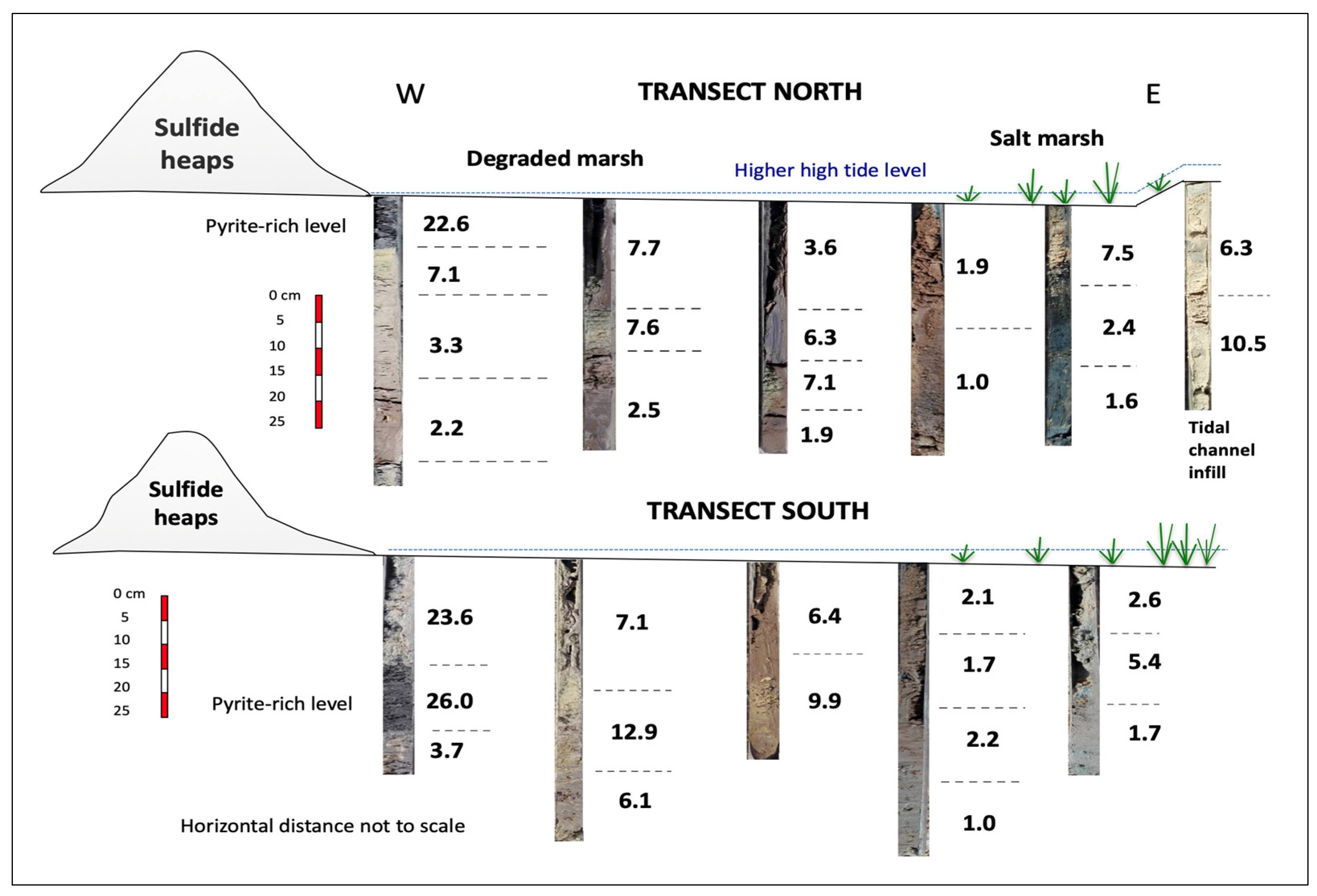
Given the polymetallic nature of the contamination, a quantitative evaluation of the multielement soil anomalies was made based on the pollution load index of Tomlinson et al. [24] by taking the seven highest enriched elements (As, Cd, Cu, Pb, Sb, Tl, and Zn) and deriving the seventh root of the seven contamination factors multiplied together (Equation (2)). The PLI values were highly variable both laterally and vertically over the investigated zones (Figure 9). In fact, the metal loading of the soil differed noticeably from one sampling site to another, and even within the same core. The highest metal loading was recorded at the yellow zone immediately adjacent to the sulphide heaps, not only in the topsoil (PLI = 23.6) but also in the subsoil (PLI = 26.0) due to the deposition of pyrite grains carried from the stockpiles by past runoff events. Jarosite seems to be responsible for the high PLI values observed in the furthest yellow zone. On the contrary, the PLI values recorded at the deepest sampling levels of the distal areas were close to unity, except for the jarosite-rich channel infill, where the PLI values were between 6.3 and 10.5.
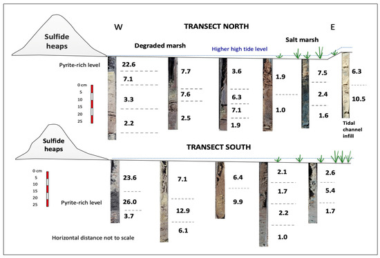
Figure 9.
Pollution load index (PLI) values of the soil core samples.
5.4. Potential Human Health and Ecological Risks
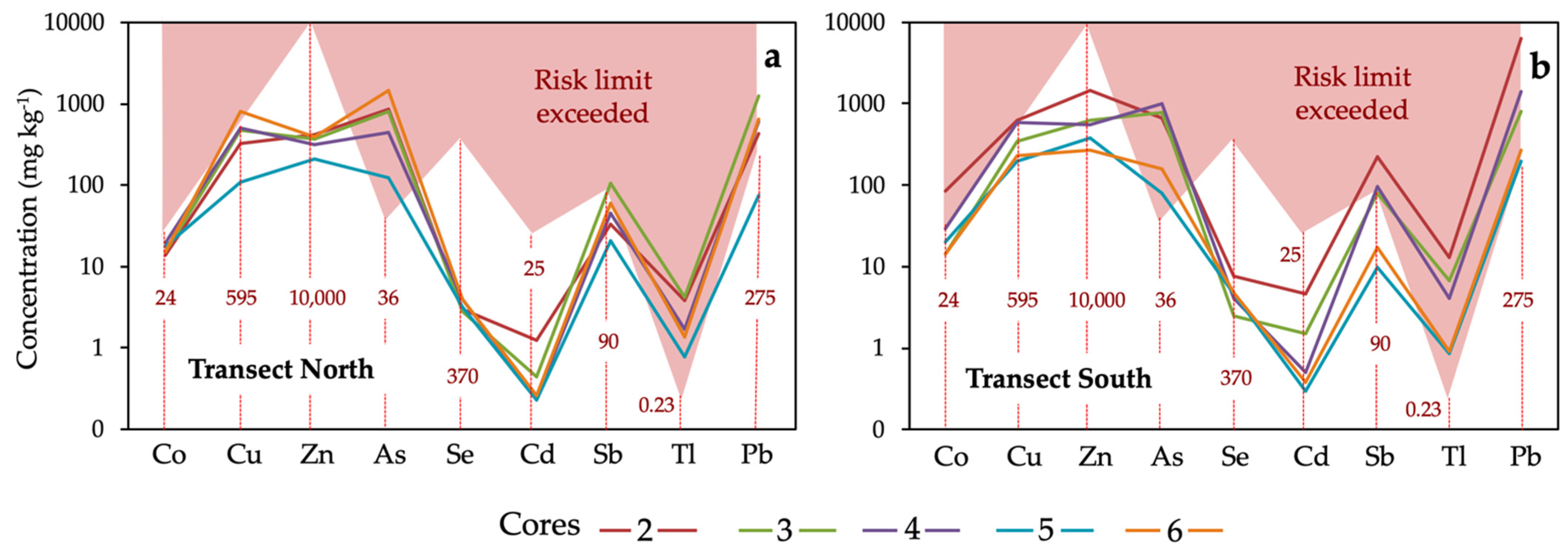
The presence of anthropogenic PTEs at concentrations above certain thresholds can pose an unacceptable risk to human health and surrounding ecosystems. For screening purposes, the median concentration of each PTE was compared to its generic reference level (Figure 10), which is statutorily defined as the concentration of a contaminant that does not result in a level of risk higher than the maximum acceptable limits for human health or ecosystems [14].
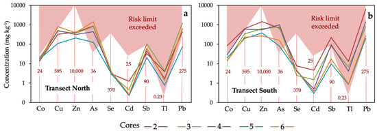
Figure 10.
Median concentrations of trace elements in the soil cores collected in each sampling site of the north transect (a) and south transect (b). The red dashed vertical lines indicate the regulatory guidance values for soils of southern Spain [46], above which adverse effects on human health may occur.
The results show that the concentrations of As, Tl, and Pb in soil throughout the transects are well above the regulatory levels established for wetland use, reaching values above which adverse health effects may potentially occur. The Tl content in the sample 2b from the southern transect exceeded 100 times the guidance value. Consequently, the soil should be declared as polluted according to the Spanish regulatory framework, which was implemented following the guideline of the European Directive 2008/98/EC. The maximum allowable concentrations of Cu, Sb and Co were also exceeded in some samples. By contrast, the level of risk associated with exposure to the other anthropogenic PTEs (Zn, Cd and Se) is expected to be acceptable because their concentrations fell within the regulatory threshold values in all sampling locations.
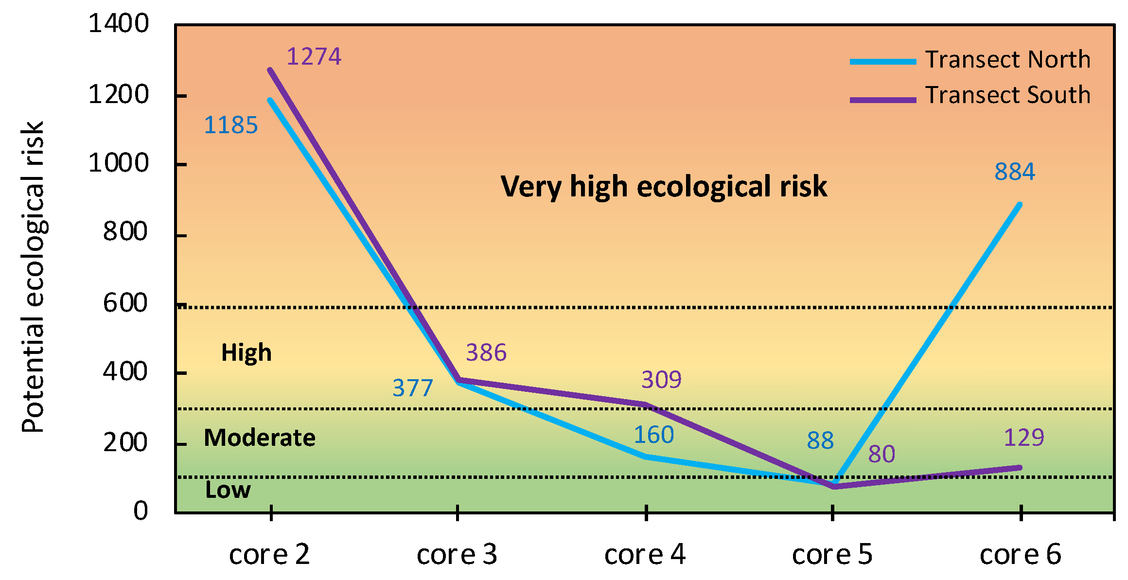
The ERI values were highly variable across the study area (Figure 11), ranging from 1185–1274 (very high ecological risk) in the vicinity of the sulphide heaps to 80–88 (low ecological risk) in the ochre zone. Interestingly, the surface soil collected in the sampling site 5a (ochre zone) of the transect north had an ERI value as high as 884, indicating very high ecological risk for the wetland, because the tidal channels drain the jarositic yellow zone and spread PTEs to distal areas.
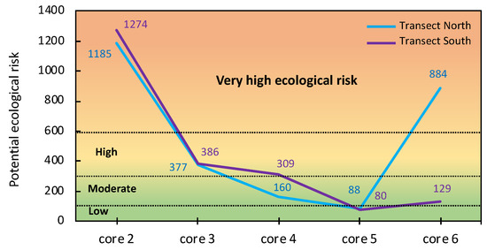
Figure 11.
Potential ecological risk values of As, Cd, Cu, Pb, and Zn in the surface samples of the soil cores collected in each transect.
Apart from the concerns arising from exposure to soil contaminants, the efflorescent minerals are vulnerable to wind erosion and may contaminate the environment and affect human health [47]. By dissolving in the humid environment of the respiratory system, the readily soluble salts may enter directly into the bloodstream and cause potential health problems to nearby residential receptors [48]. It is important to note, therefore, that the concentrations of PTEs, notably Cu and Zn, detected in the efflorescent sulphates make these transient minerals potentially toxic through airborne respirable particles.
6. Concluding Recommendations
This study has highlighted that the soil composition, properties and functions of the wetland area surrounding the mine wastes disposal site have been strongly disturbed by the detrimental long-term effects of uncontrolled sulphide oxidation. As a result of leachate generation and metal release, the receiving soil is ultra-acidic and extremely enriched in Pb, Sb, Tl, As, Cd, Zn, and Cu. In distal locations (>120 m away from the sulphide heaps) and with depth, the soil becomes moderately acidic and PTE concentrations fall within the local baseline, suggesting that metal attenuation processes are occurring by precipitation of secondary minerals (mainly iron sulphates and oxyhydroxides) related to neutralization, oxidation, and dehydration reactions.
However, based on the current status of soil contamination, the pollutants may pose an unacceptable risk to human and ecological receptors associated with potential exposure to soil minerals and wind-blown dust. In the light of this conclusion, urgent remedial work is needed to reclaim the contaminated land to a public health safety and sustainable environmental quality, and restore wetland ecosystem services. The reclamation plan should include extensive clean-up operations to remove sulphide waste, the degraded soil to a depth of about 50 cm, and the tidal channel infill. Additional soil remediation will be necessary in order to neutralize both active and exchangeable acidity and prevent mobilization and dispersal of residual metals.
Supplementary Materials
The following are available online at https://www.mdpi.com/article/10.3390/app12010249/s1, Figure S1: Schematic depiction of the soil sections from the extracted core samples; Table S1: Abbreviations and chemical formulae of minerals.
Author Contributions
The authors (M.M.G. and J.C.F.-C.) have contributed equally to the paper. All authors have read and agreed to the published version of the manuscript.
Funding
This work has been partially supported by the Andalusian Regional Government through the Research Group on Geology and Environmental Geochemistry (RNM-347).
Institutional Review Board Statement
Not applicable.
Informed Consent Statement
Not applicable.
Data Availability Statement
The authors confirm that the data supporting the findings of this study are available within the manuscript and its Supplementary Material.
Acknowledgments
We thank Jesús de la Rosa (University of Huelva) for his collaboration during fieldwork and for assistance with chemical analysis.
Conflicts of Interest
The authors declare no conflict of interest.
References
- Salomons, W. Environmental impact of metals derived from mining activities: Processes, predictions, prevention. J. Geochem. Explor. 1995, 52, 5–23. [Google Scholar] [CrossRef]
- Hudson-Edwards, K. Tackling mine wastes. Science 2016, 352, 288–290. [Google Scholar] [CrossRef]
- Olías, M.; Nieto, J.M.; Sarmiento, A.M.; Cerón, J.; Canovas, C.R. Seasonal water quality variations in a river affected by acid mine drainage: The Odiel River (South West Spain). Sci. Total Environ. 2004, 333, 267–281. [Google Scholar] [CrossRef]
- Sánchez-España, J.; Pamo, E.L.; Pastor, E.S.; Andrés, J.R.; Rubí, J.A.M. The Impact of Acid Mine Drainage on the Water Quality of the Odiel River (Huelva, Spain): Evolution of Precipitate Mineralogy and Aqueous Geochemistry along the Concepción-Tintillo Segment. Water Air Soil Pollut. 2006, 173, 121–149. [Google Scholar] [CrossRef]
- Blowes, D.W.; Ptacek, C.J.; Jambor, J.L.; Weisener, C.G. The geochemistry of acid mine drainage. In Treatise on Geochemistry; Elsevier: Amsterdam, The Netherlands, 2003; pp. 149–204. ISBN 978-0-08-043751-4. [Google Scholar]
- Plumlee, G.S.; Morman, S.A. Mine Wastes and Human Health. Elements 2011, 7, 399–404. [Google Scholar] [CrossRef]
- Candeias, C.; Da Silva, E.F.; Salgueiro, A.R.; Pereira, H.G.; Reis, A.P.; Patinha, C.; Matos, J.X.; Ávila, P.H. Assessment of soil contamination by potentially toxic elements in the aljustrel mining area in order to implement soil reclamation strategies. Land Degrad. Dev. 2010, 22, 565–585. [Google Scholar] [CrossRef] [Green Version]
- Fernández-Caliani, J.C.; Barba-Brioso, C.; González, I.; Galán, E. Heavy Metal Pollution in Soils Around the Abandoned Mine Sites of the Iberian Pyrite Belt (Southwest Spain). Water Air Soil Pollut. 2008, 200, 211–226. [Google Scholar] [CrossRef]
- Fernández-Caliani, J.C.; Giráldez, M.I.; Barba-Brioso, C. Oral bioaccessibility and human health risk assessment of trace elements in agricultural soils impacted by acid mine drainage. Chemosphere 2019, 237, 124441. [Google Scholar] [CrossRef] [PubMed]
- Nordstrom, D.K.; Alpers, C.N. Geochemistry of acid mine waters. In The Environmental Geochemistry of Mineral. Deposits. Part A: Processes, Techniques, and Health Issues; Plumlee, G.S., Logsdon, M.J., Eds.; Society of Economic Geologists: Littleton, CO, USA, 1997; pp. 133–160. [Google Scholar] [CrossRef]
- Somma, R.; Ebrahimi, P.; Troise, C.; De Natale, G.; Guarino, A.; Cicchella, D.; Albanese, S. The first application of compositional data analysis (CoDA) in a multivariate perspective for detection of pollution source in sea sediments: The Pozzuoli Bay (Italy) case study. Chemosphere 2021, 274, 129955. [Google Scholar] [CrossRef]
- Buccino, M.; Daliri, M.; Calabrese, M.; Somma, R. A numerical study of arsenic contamination at the Bagnoli bay seabed by a semi-anthropogenic source. Analysis of current regime. Sci. Total Environ. 2021, 782, 146811. [Google Scholar] [CrossRef]
- Fernández-Caliani, J.C.; Grantcharova, M.M. Enrichment and Fractionation of Rare Earth Elements in an Estuarine Marsh Soil Receiving Acid Discharges from Legacy Sulfide Mine Wastes. Soil Syst. 2021, 5, 66. [Google Scholar] [CrossRef]
- Tarazona, J.V.; Fernández, M.D.; Vega, M.M. Regulation of Contaminated Soils in Spain—A New Legal Instrument (4 pp). J. Soils Sediments 2005, 5, 121–124. [Google Scholar] [CrossRef]
- Fernández-Caliani, J.C. Risk-based assessment of multimetallic soil pollution in the industrialized peri-urban area of Huelva, Spain. Environ. Geochem. Health 2011, 34, 123–139. [Google Scholar] [CrossRef]
- Jerz, J.K.; Rimstidt, J.D. Efflorescent iron sulfate minerals: Paragenesis, relative stability, and environmental impact. Am. Miner. 2003, 88, 1919–1932. [Google Scholar] [CrossRef]
- World Reference Base for Soil Resources 2014; World Soil Resources Reports 106; FAO: Rome, Italy, 2015; Available online: www.fao.org/3/i3794en/I3794en.pdf (accessed on 1 December 2021).
- Finkl, C.W.; Makowski, C. (Eds.) Coastal Wetlands: Alteration and Remediation; Springer: Cham, Switzerland, 2017; Volume 2. [Google Scholar] [CrossRef] [Green Version]
- Zhou, X.; Liu, D.; Bu, H.; Deng, L.; Liu, H.; Yuan, P.; Du, P.; Song, H. XRD-based quantitative analysis of clay minerals using reference intensity ratios, mineral intensity factors, Rietveld, and full pattern summation methods: A critical review. Solid Earth Sci. 2018, 3, 16–29. [Google Scholar] [CrossRef]
- Barbieri, M. The Importance of Enrichment Factor (EF) and Geoaccumulation Index (Igeo) to Evaluate the Soil Contamination. J. Geol. Geophys. 2016, 5, 1–4. [Google Scholar] [CrossRef]
- Kowalska, J.B.; Mazurek, R.; Gąsiorek, M.; Zaleski, T. Pollution indices as useful tools for the comprehensive evaluation of the degree of soil contamination–A review. Environ. Geochem. Health 2018, 40, 2395–2420. [Google Scholar] [CrossRef] [Green Version]
- Varol, M.; Sünbül, M.R.; Aytop, H.; Yılmaz, C.H. Environmental, ecological and health risks of trace elements, and their sources in soils of Harran Plain, Turkey. Chemosphere 2019, 245, 125592. [Google Scholar] [CrossRef]
- Salomons, W.; Förstner, U. Metals in the Hydrocycle; Springer: Berlin/Heidelberg, Germany, 1984. [Google Scholar] [CrossRef]
- Tomlinson, D.L.; Wilson, J.G.; Harris, C.R.; Jeffrey, D.W. Problems in the assessment of heavy-metal levels in estuaries and the formation of a pollution index. Helgoländer Meeresunters. 1980, 33, 566–575. [Google Scholar] [CrossRef] [Green Version]
- Håkanson, L. An ecological risk index for aquatic pollution control: A sedimentological approach. Water Res. 1980, 14, 975–1001. [Google Scholar] [CrossRef]
- Müller, G. Index of geoaccumulation in sediments of the Rhine River. J. Geol. 1969, 2, 108–118. [Google Scholar]
- Jambor, J.L.; Nordstrom, D.K.; Alpers, C.N. Metal-sulfate salts from sulfide mineral oxidation. Rev. Mineral. Geochem. 2000, 40, 303–350. [Google Scholar] [CrossRef]
- Singer, P.C.; Stumm, W. Acidic Mine Drainage: The Rate-Determining Step. Science 1970, 167, 1121–1123. [Google Scholar] [CrossRef]
- Rimstidt, J.; Vaughan, D.J. Pyrite oxidation: A state-of-the-art assessment of the reaction mechanism. Geochim. Cosmochim. Acta 2003, 67, 873–880. [Google Scholar] [CrossRef]
- Davila, J.M.; Sarmiento, A.M.; Santisteban, M.; Luís, A.; Fortes, J.C.; Diaz-Curiel, J.; Valbuena, C.; Grande, J.A. The UNESCO national biosphere reserve (Marismas del Odiel, SW Spain): An area of 18,875 ha affected by mining waste. Environ. Sci. Pollut. Res. 2019, 26, 33594–33606. [Google Scholar] [CrossRef]
- Rimstidt, J.D.; Chermak, J.A.; Gagen, P.M. Rates of Reaction of Galena, Sphalerite, Chalcopyrite, and Arsenopyrite with Fe(III) in Acidic Solutions; ACS Symposium Series. In Environmental Geochemistry of Sulfide Oxidation; Alpers, C.N., Blowes, D.W., Eds.; American Chemical Society: Washington, DC, USA, 1994; Volume 1, pp. 2–13. [Google Scholar] [CrossRef] [Green Version]
- Abbassi, R.; Khan, F.; Hawboldt, K. Prediction of Minerals Producing Acid Mine Drainage Using a Computer-Assisted Thermodynamic Chemical Equilibrium Model. Mine Water Environ. 2009, 28, 74–78. [Google Scholar] [CrossRef]
- España, J.S.; Pamo, E.L.; Santofimia, E.; Aduvire, O.; Reyes-Andrés, J.; Barettino, D. Acid mine drainage in the Iberian Pyrite Belt (Odiel river watershed, Huelva, SW Spain): Geochemistry, mineralogy and environmental implications. Appl. Geochem. 2005, 20, 1320–1356. [Google Scholar] [CrossRef]
- Hammarstrom, J.; Seal, R.; Meier, A.; Kornfeld, J. Secondary sulfate minerals associated with acid drainage in the eastern US: Recycling of metals and acidity in surficial environments. Chem. Geol. 2005, 215, 407–431. [Google Scholar] [CrossRef] [Green Version]
- Asta, M.P.; Cama, J.; Martinez, M.; Giménez, J. Arsenic removal by goethite and jarosite in acidic conditions and its environmental implications. J. Hazard. Mater. 2009, 171, 965–972. [Google Scholar] [CrossRef]
- Aguilar-Carrillo, J.; Herrera-García, L.; Reyes-Domínguez, I.A.; Gutiérrez, E.J. Thallium(I) sequestration by jarosite and birnessite: Structural incorporation vs. surface adsorption. Environ. Pollut. 2019, 257, 113492. [Google Scholar] [CrossRef]
- Bigham, J.M.; Nordstrom, D.K. Iron and Aluminum Hydroxysulfates from Acid Sulfate Waters. Rev. Miner. Geochem. 2000, 40, 351–403. [Google Scholar] [CrossRef]
- Bigham, J.; Schwertmann, U.; Traina, S.; Winland, R.; Wolf, M. Schwertmannite and the chemical modeling of iron in acid sulfate waters. Geochim. Cosmochim. Acta 1996, 60, 2111–2121. [Google Scholar] [CrossRef]
- Schwertmann, U.; Carlson, L. The pH-dependent transformation of schwertmannite to goethite at 25°C. Clay Miner. 2005, 40, 63–66. [Google Scholar] [CrossRef]
- Alpers, C.N.; Blowes, D.W.; Nordstrom, D.K.; Jambor, J.L. Secondary minerals and acid mine-water chemistry. In Environmental Geochemistry of Sulfide Mine-Wastes; Blowes, D.W., Jambor, J.L., Eds.; Mineralogical Association of Canada, Short Course Handbook: Quebec, QC, Canada, 1994; Volume 22, pp. 247–270. [Google Scholar]
- Buckby, T.; Black, S.; Coleman, M.; Hodson, M. Fesulphate-rich evaporative mineral precipitates from the Río Tinto, southwest Spain. Miner. Mag. 2003, 67, 263–278. [Google Scholar] [CrossRef]
- Romero-Baena, A.J.; González, I.; Galan, E. The Role of Efflorescent Sulfates in The Storage of Trace Elements in Stream Waters Polluted by Acid Mine-Drainage: The Case of Pena Del Hierro, Southwestern Spain. Can. Miner. 2006, 44, 1431–1446. [Google Scholar] [CrossRef]
- Iriarte, A.; Iriarte, P.I.; Bouza, P.J.; Martín, F. Los Suelos del Entorno de la Ría de Huelva; Consejería de Medio Ambiente de la Junta de Andalucía: Seville, Spain; Consejo Superior de Investigaciones Científicas: Madrid, Spain, 2007. [Google Scholar]
- Galán, E.; Fernandez-Caliani, J.C.; González, I.; Aparicio, P.; Romero, A. Influence of geological setting on geochemical baselines of trace elements in soils. Application to soils of South–West Spain. J. Geochem. Explor. 2008, 98, 89–106. [Google Scholar] [CrossRef]
- Abrahim, G.M.S.; Parker, R.J. Assessment of heavy metal enrichment factors and the degree of contamination in marine sediments from Tamaki Estuary, Auckland, New Zealand. Environ. Monit. Assess. 2007, 136, 227–238. [Google Scholar] [CrossRef] [PubMed]
- de Andalucía, J. Decreto 18/2015, de 27 de enero, por el que se aprueba el reglamento que regula el régimen aplicable a los suelos contaminados. Boletín Oficial de la Junta de Andalucía 2015, 38, 28–64. [Google Scholar]
- Meza-Figueroa, D.; Maier, R.; de la O-Villanueva, M.; Gómez-Alvarez, A.; Moreno-Zazueta, A.; Rivera, J.; Campillo, A.; Grandlic, C.J.; Anaya, R.; Palafox-Reyes, J. The impact of unconfined mine tailings in residential areas from a mining town in a semi-arid environment: Nacozari, Sonora, Mexico. Chemosphere 2009, 77, 140–147. [Google Scholar] [CrossRef] [PubMed] [Green Version]
- Loredo-Jasso, A.U.; Villalobos, M.; Ponce-Pérez, D.B.; Pi-Puig, T.; Meza-Figueroa, D.; del Rio-Salas, R.; Ochoa-Landín, L. Characterization and pH neutralization products of efflorescent salts from mine tailings of (semi-)arid zones. Chem. Geol. 2021, 580, 120370. [Google Scholar] [CrossRef]


Publisher’s Note: MDPI stays neutral with regard to jurisdictional claims in published maps and institutional affiliations. |
© 2021 by the authors. Licensee MDPI, Basel, Switzerland. This article is an open access article distributed under the terms and conditions of the Creative Commons Attribution (CC BY) license (https://creativecommons.org/licenses/by/4.0/).