
Dynamics Investigation on Axial-Groove Gas Bearing-Rotor System with Rod-Fastened Structure


1
School of Mechanical and Precision Instrument Engineering, Xi’an University of Technology, Xi’an 710048, China
2
State Key Laboratory for Manufacturing Systems Engineering, Xi’an Jiaotong University, Xi’an 710049, China
3
Faculty of Printing, Packaging Engineering and Digital Media Technology, Xi’an University of Technology, Xi’an 710054, China
4
School of Railway Power, Shaanxi Railway Institute, Weinan 714000, China
*
Author to whom correspondence should be addressed.
Appl. Sci. 2022, 12(1), 250; https://doi.org/10.3390/app12010250
Submission received: 30 November 2021
/
Revised: 20 December 2021
/
Accepted: 21 December 2021
/
Published: 28 December 2021
(This article belongs to the Special Issue Nonlinear Analysis of Static and Dynamic Problems in Mechanical Engineering)
Abstract
:This research report discusses the dynamic behaviors of an axial-groove gas bearings-rotor system with rod-fastened structure. The time-based dependency-compressible Reynolds equation in the gas bearing nonlinear system is solved by the differential transformation method, and the continuous gas film forces of a three-axial-groove gas bearing are obtained. A dynamic mathematical model of the rotor system with rod-fastened structure supported in two- and three-axial-groove gas bearings with eight degrees of freedom is established. The dynamic motion equation of the rod-fastened rotor system is solved by the modified Newmark-β method based on disturbance compensation, which can reduce the computing error and improve computing stability. The dynamic characteristics of the rod-fastened rotor-gas bearing system are analyzed efficiently by the diversiform unbalance responses. The influence of the position angle of the pad on the nonlinear characteristics of the rod-fastened rotor system is also studied.
1. Introduction
Oil-free lubrication provides many unique characteristics for gas bearings, such as low friction, high positioning precision and low pollutant emission. As a result, the rotor system supported in a gas bearing is frequently employed within the high-speed rotating machinery, whether in civilian, agriculture, or military aerospace fields. The characteristic of rotor dynamics is one key factor for the stable operation of high-speed rotating machinery. It is necessary to carry out more research about the stability analysis and dynamic performance of the gas bearing-rotor system [1,2,3,4].
Li et al. [5] studied the effects of the circumferential and axial surface waviness on the nonlinear dynamic characteristics of a gas-lubricated bearing-rotor system; the dynamic stability of the bearing-rotor system can be improved with the increase of amplitude of circumferential waviness. Based on the finite difference method, perturbation method, and mixing method, Wang et al. [6] investigated the nonlinear dynamic performance of the flexible rotor system with opposed high-speed gas bearing support; by changing the parameters of the bearing, chaos phenomena and the system loss produced by the irregular vibration can be reduced. Yang et al. [7] analyzed numerically the unbalance response and dynamic stability of the rotor system supported on a micro gas bearing with a gas rarefaction effect; the influence of mass eccentricities of rotor on the stability of rotor system supported on the micro gas bearing was discussed. Wang et al. [8] analyzed the nonlinear dynamic behavior of a hybrid active aerostatic and aerodynamic bearing-rotor system by using a mixed numerical method, and the complex dynamic phenomena under different parameters and conditions were obtained. These gas bearings are cylindrical bearings, which have a simple structure and high-load-carrying capacity, but the rotor system supported by the cylindrical gas bearing is prone to instability under higher speed. The application of grooved gas bearings ensures the stable operation and improves the work performance of high-speed machinery; many research results were obtained on the lubrication performance of the grooved bearings. Feng et al. [9] focused on gas bearings with a micro spherical spiral groove, and the thermohydrodynamic performance of the bearings was analyzed by considering the surface roughness and air rarefaction, the effects of surface roughness and slip flow were obtained by using the Weierstrass–Mandelbrot function and Wu’s slip model. Zhang et al. [10] studied the contact characteristics of a gas-lubricated thrust micro-bearing with a spiral-groove by considering the gas rarefaction, and the effects of the standard deviation of asperity height and the groove depth on the surface contact forces of the gas-lubricated bearing were discussed. Jia et al. [11,12] built a mathematical model of spherical spiral-groove hybrid-gas bearings rotor system coupled with the analysis of nonlinear dynamic lubrication. The critical speed of the rotor-bearing system was calculated and the stability of the hybrid gas bearings was predicted; they then forced the dynamic variation rule of the gas film damping and stiffness under different states of motion, and the vortex motion and oscillation phenomenon of the gas film was analyzed. Liu et al. [13] studied the nonlinear dynamic characteristics of a rigid rotor system with herringbone-grooved-journal gas bearings support, the onset speed and the whirl frequency ratio of subsynchronous vibration in the gas bearings-rotor system were estimated and analyzed. Du et al. [14] investigated the whirl motion of a rigid rotor system with spiral-grooved opposed-hemisphere gas bearing support; the complicated rotor responses under the initial disturbance were analyzed, and the synchronous and nonsynchronous excitations were obtained. Based on time delays and feedback control gains, the dynamic behavior of the rotor supported by the self-acting three-axial-grooved gas-lubricated bearings were investigated by us [15], and a mathematical method used to obtain the dynamic characteristics of the nonlinear gas bearing-rotor system is presented. The unbalanced responses of a rigid rotor system supported by two-axial-groove gas bearings were analyzed by us [16]; a numerical model was established and utilized to acquire the rich nonlinear phenomena.
Continuous rotor models have been investigated thoroughly in rotor-gas bearing systems [5,6,7,8,11,12,13,14,15,16]. Li et al. [17] analyzed the rotor vibration characteristics of a gas bearing-rotor system, jointed by bolted-disk, by considering dynamic parameters of bolted-disk joints. Using the changes of the bending stiffness and tangential stiffness of the bolted-disk joints, the dynamic vibration characteristics of the rotor system were analyzed. An improved integrated modal technique with a free interface for reducing the number of degrees of freedom of a continuous flexible rotor system was presented by us [18]. The nonlinear dynamic behavior of a continuous rotor with multi-span bearing support was investigated by our proposed method. Chasalevris and Papadopoulos [19] proposed a new semi-analytical method for simulating the dynamic response of multi-segment continuous rotor bearing systems. Yang et al. [20] numerically suppressed the unbalance responses of the continuous flexible rotor systems supported on the tilting-pad gas bearings by using the proportional-derivative control model. Compared with the continuous rotors, the rod-fastened rotors are widely used to adapt the actual working conditions in the aircraft engine and gas turbines. Because of the effects of contacts among the components, the dynamic characteristics of the rod-fastened rotor have been studied increasingly. Liu et al. [21] proposed a method for investigating the dynamic stability and bifurcation behaviors of the rod fastening rotor and complete bearing system. The comparison results of the periodic motions and stability conditions in the rod fastening and continuous rotor-bearings system indicated that their bifurcation characteristics have a general resemblance. Wu et al. [22] built a mechanical model of a rod fastening rotor-bearing system by considering the contact effect between the disks. To characterize the contact interface, a nonlinear stiffness matrix containing stiffness coefficients was presented. Li et al. [23] studied the dynamic characteristics of an air bearing-rod fastening rotor system, which considered the heterogeneous bending stiffness of the contact interface; the linear and nonlinear dynamics behaviors were obtained. Wang et al. [24] analyzed the effects of the internal damping of a rod-fastened rotor-bearing nonlinear system on the dynamic responses and rotor stability. With the effect of internal damping, the amplitudes of dynamic response were decreased to some extent at lower speed and amplified significantly at higher speed. The dynamic responses and bifurcation phenomenon of a rod-fastened rotor supported by a fixed-tilting pad gas bearing were investigated by us [25]. The periodic orbits, pendulum angles, and Poincaré map with the different pad pivot ratios and preloads for the symmetrical and asymmetrical rotor-bearing system were analyzed. Our results showed that the rod-fastened rigid rotor system has better stability than the continuous integral rotor system. Hu et al. [26,27] investigated dynamic characteristics of the rod-fastened rotor bearing system, considering the rub-impact effect and influence of rotating velocities and radial stiffnesses of stator. Based on the D’Alembert principle, a nonlinear dynamic hybrid model of the rod-fastened rotor was built by considering different rub-impact and initial permanent deflection; the effects of rotating speed and the length of initial permanent deflection on the dynamic behaviors of the journal bearing rod-fastened rotor system were analyzed.
A dynamic mathematical model of a rotor system with a rod-fastened structure supported on three-axial-groove gas bearings is formulated in this report. The time-based dependency-compressible Reynolds equation in the gas bearing lubrication nonlinear system is solved by using the differential transformation method, and the nonlinear gas film forces of a three-axial-groove gas bearing are obtained. The eight degrees of freedom dynamic motion equation of the rod-fastened rotor-gas bearing system is solved by the modified Newmark-β method, which considers the disturbance compensation. The dynamic behaviors of the rod-fastened rotor-bearing nonlinear system are analyzed efficiently, and the dynamic unbalance responses of the rod-fastened rotor and continuous integral rotor, three-axial-grooved and two-axial-grooved gas bearings are compared. Furthermore, the effects of the position angle of the pad on the nonlinear dynamic behavior are also investigated.
2. Kinematic Model and Mathematical Method of Three-Axial-Groove Gas Bearing
2.1. Kinematic Model
The axial-groove gas bearing and the coordinate system are shown in Figure 1. Axial grooves are distributed uniformly in the circumferential direction. xOby denotes the bearing coordinate system; Ob denotes the bearing center of the axial-groove gas bearing; Oj denotes the journal center; ϕ denotes the angle which is from the negative y direction to the gas film position along the rotating direction; e denotes the eccentricity of the gas bearing; ω denotes the rotation angular speed; Rb denotes the gas bearing radius; c denotes the radial clearance; α denotes the angle of groove width; α0 denotes the angle from leading edge of the pad to the negative y direction; β denotes the arc bushing angle of the single pad; and Fx and Fy denote the gas film forces of the coordinate system xOby in the x and y directions.
In order to obtain the gas film forces Fx, Fy of the axial-groove gas bearing, the gas pressure p needs to be calculated by solving the compressible Reynolds equation. Reynolds equation is the theoretical basis of fluid lubricated bearing research, which depicts the relationship between the gas pressure and gas thickness. Considering a gas journal bearing, the compressible lubrication Reynolds equation is:
where p denotes the gas film pressure in the coordinate system; h denotes the gas film thickness, for the ith pad, hi = 1 + eicos(ϕ − θi); z denotes the coordinate in the axial direction; x denotes the angle from the line of centers Oj and Ob to the gas film current position in the circumferential direction; μ denotes the average velocity of the gas; and U denotes the component of velocity in the x direction.
The dimensionless procedure is applied to Equation (1) by using the following transformational relations: p = P × Pa, h = H × c, z = λ × Rb, x = φ × Rb, τ = t × ω, U = ω × R. A unified equation can be then obtained as follows:
where Λ = 6μωR2/(Pac2) and denotes the bearing number of the gas bearing.
For Equation (2), the boundary conditions are:
- The gas film pressures at the both ends of bearing: P (φ, Bb/2Rb) = P (φ, −Bb/2Rb) = 1;
- The gas film pressures at the leading edge (φi1) and trailing edge (φi2) of single pad in the axial direction: P (φ1, λ) = P (φ2, λ) = 1.
By using the differential transformation method, the dimensionless Reynolds equation is solved efficiently.
2.2. Mathematical Method of Nonlinear Gas Film Force
The differential transformation method [28,29] has significant merits; rapid convergence can be achieved and the computational error can be reduced. The time is discretized in the nonlinear Reynolds equation by the differential transformation method. The gas film pressure P is a time-dependent function in the time domain, and the differential transform of the kth derivative of the gas film pressure P(t) can be expressed as:
where Pt(k) denotes the transform function in the transform domain. The differential inverse transform Pt(k) can be written as:
where T denotes the time gap. While the value P(0) (k = 0) is known, Pt (0) can be obtained by Equation (4), and then the other discrete value P(k) can be obtained in the time interval T.
By using the differential transformation method, the compressible Reynolds equation of the axial-groove gas bearing can be solved, and the transform with respect to the time domain τ is made.
Introducing , , and , S(k) denotes the differential transform of P2. I(k) and J(k) denote the differential transforms of H2 and H3. The differential transformation of Equation (2) can be written as:
where denotes the convolution operator.
Equation (5) is discretized in the circumferential and axial directions by the central difference method. The discretized equation can be obtained:
where Δφ and Δλ denote the steps in the circumferential and axial directions; Δτ denotes the time step; k, m and n denote the differential transformation orders (k ≥ m ≥ n); and i and j denote the coordinates of the nodal position in the φ and λ directions.
Because the centerline of the journal is parallel to the centerline of the gas bearing, the gas film thickness is constant in the λ direction, i.e., ∂λHi,j = 0. When k = m = n = 0, Equation (6) can be transformed as:
Si,j(0), Ii,j (0), and Ji,j (0) are expressed as:
where Hi(0) denotes the gas film thickness in the last moment and Pi,j(0) denotes the gas film pressure in the last moment.
By substituting Equation (8) into Equation (7), Equation (9) follows:
where Hi(1) and Pi,j(1) denote the relevant variables of the thickness and pressure of the gas film in the time interval τ.
When k = 1, then m = n = 0 and Equation (6) can be written as:
Si,j(1), Ii,j (1), and Ji,j (1) can be expressed as:
By substituting Equations (8) and (11) into Equation (10), one can obtain:
By substituting Hi(0), Pi,j(0), and Hi(1) into Equations (9) and (12), Pi,j (1) can be calculated from Equation (9) and Pi,j (2) can be calculated from Equation (12). Pi,j is calculated in the following form:
The calculation flow chart of the differential transform method is shown in Figure 2.
3. Dynamic Model and Method of the Rod-Fastened Rotor-Gas Bearing System
3.1. Dynamic Motion of the Rod-Fastened Rotor-Gas Bearing System
The rod-fastened rotor-gas bearing system is depicted in Figure 3. The rod-fastened rotor consists of shafts, disks, and gas bearings. Two rigid disks are bolted by rods, which are circumferentially distributed on the disk. The mass and damping of the rod are ignored when it is equivalent to a nonlinear stiffness spring structure. The rod-fastened rotor is supported by two- and three-axial-groove gas bearings, and the mass of the axial-groove gas bearing is not considered. In Figure 3a, O1 and O2 denote the journal centers at the left- and right-bearing stations, respectively; m1 and m2 denote the lumped masses of the left and right segments, respectively; l1 and l2 denote the lengths of the left and right segments, respectively; Od1 and Od2 denote the centers of the rigid disks, respectively; and md1 and md2 denote the masses of two rigid disks, respectively. Figure 3b shows the circumferential distribution of the rods; Rd denotes the radius of rigid disks.
The dynamic motion model of the rod-fastened rotor system with two- and three-axial-groove gas bearings support follows:
where u = [x1, y1, x2, y2, xd1, yd1, xd2, yd2]T; M denotes the mass matrix of the dynamic motion; K denotes the stiffness matrix; and P denotes the dynamic resultant force matrix.
where fx and fy denote the gas film forces of the axial-groove gas bearing, respectively; ed1 and ed1 are the mass eccentricities of the rigid disks, respectively; xd1 and yd1 denote the displacements of disk 1 in the x and y directions, respectively; xd2 and yd2 denote the displacements of disk 2 in the x and y directions, respectively; k1 and k2 denote the bending stiffnesses of the left and right segments, respectively; kb denotes the bending stiffness of the bolted rod; frx1 and fry1 denote the restoring forces of the disk 1, respectively; frx2 and fry2 denote the restoring forces of the disk 2, respectively; and kr denotes the restoring stiffness.
where xr1, yr1, xr1, and yr1 denote the motion displacements of disk centers in the x and y directions in the last moment.
The dynamic motion model of the rod-fastened rotor system can be solved by using the Newmark-β method; however, calculation errors may occur while a disturbance is produced by an increment of acceleration.
3.2. Newmark-β Method Based on Disturbance Compensation
For solving the dynamic motion model of the rod-fastened rotor-gas bearing system efficiently, the modified Newmark-β method is employed by considering the disturbance compensation. The Newmark-β method is based on the average constant acceleration theory; that is, the acceleration is assumed to be a constant between and . The integration constants of Newmark-β method are given in Table 1.
For the equation of motion, the dynamic response equation at time step t = iτ is expressed as follows:
where and denote the acceleration and displacement at time step iτ. By the average constant acceleration theory, the average constant acceleration can be obtained as , which is between previous time step (i − 1)τ and time step iτ, denotes the acceleration at previous time step (i − 1)τ. denotes the acceleration at time iτ; and can be written as:
where and are the velocity and displacement at the previous time step (i − 1)τ. According to Equation (20), can be written as:
By substituting Equations (21) and (22) into Equation (19), the equivalent motion Equation (23) can be obtained:
where denotes the equivalent stiffness matrix, which does not change with time; denotes the equivalent dynamic resultant force matrix which is relevant to time.
The displacement at time iτ can be obtained by solving Equation (23).
According to the constrained condition of motion, the , , and are obtained by the Newmark-β method, but according to the dynamic motion equation, the actual acceleration is obtained by substituting and into Equation (19).
It can be seen that an increment of acceleration at time step iτ is produced as Equation (28), which produces a disturbance error at each time step. By substituting into Equation (27), Equation (29) can be obtained; the increment of acceleration gives rise to an increment of dynamic resultant force , which is the disturbance increment produced by the increment of acceleration .
For acquiring the displacements, velocities, and accelerations at time step t = iτ, which satisfy the constraint condition of motion and dynamic motion equation simultaneously, the increment of dynamic resultant force needs to be eliminated by the following process. According to the motion equation, an increment motion equation is established; , , and are the displacement increment, velocity increment and acceleration increment caused by , respectively, which can be obtained by Equation (30):
The displacement, velocity, and acceleration can be obtained by adding Equations (29) and (30), which are considering the incremental compensation.
The displacement , velocity and acceleration are the accurate solution of the motion equation, which take the incremental compensation into consideration in Newmark-β method. The solutions conform to the dynamic motion equation, meanwhile, satisfy the motion constraint condition of the Newmark-β method.
4. Results and Discussions
The dynamics model of the rod-fastened rotor-gas bearing system is established in Section 3.1. The geometric construction of the rod-fastened rotor system is shown in Figure 3a. The dynamic responses of the rod-fastened rotor-gas bearing system are obtained using the modified Newmark-β method, illustrated in Section 3.2. In the following, the unbalance responses of the rod-fastened rotor system with two- and three-axial-groove gas bearings support are calculated and analyzed by orbit diagrams, Poincaré maps, and spectrograms. The parameter values selected for the rod-fastened rotor and the three-axial-groove gas bearing are listed in Table 2.
4.1. Comparison of the Rod-Fastened Rotor and Continuous Integral Rotor
The orbits of the rod-fastened rotor and continuous integral rotor are compared by using the same parameter values. When ω = 1500 rad/s, Figure 4a shows the orbits comparison of the rod-fastened rotor and continuous integral rotor at the left bearing station, and Figure 4b shows the spectra of the continuous integral rotor. The dynamic response is period-doubling motion in the continuous integral rotor system, whereas, the orbit of the rod-fastened rotor is periodic motion. For the model of the gas bearing-rotor system in this report, when ω = 1500 rad/s, the unbalance responses of the rod-fastened rotor are more stable than the continuous integral rotor.
4.2. Bifurcation Characteristics
The bifurcation diagram depicts the projections of orbit of the journal center in the y direction, i.e., the y1 of the vector u = [x1, y1, x2, y2, xd1, yd1, xd2, yd2]T in Equation (14). When the rotating speed is at ω = 900~2500 rad/s, the bifurcation behavior of the rod-fastened rotor at the left bearing station are shown in Figure 5. The rod-fastened rotor system experiences quasiperiodic motion at ω = 900~1050 rad/s, and inversely bifurcates to periodic motion at ω = 1100 rad/s, and then maintains the stable motion state until ω = 1750 rad/s. When the rotating speed increases to 1775 rad/s, the response of the rod-fastened rotor-gas bearing system bifurcates to quasiperiodic motion again, and the amplitude of quasiperiodic motion increases with the amplification of the rotating speed. From the bifurcation diagram, the rod-fastened rotor-gas bearing system maintains a relatively stable operation at ω = 1100~1750 rad/s.
4.3. Unbalance Responses Versus Rotating Speed ω
At different rotating speeds, the journal center of the rod-fastened rotor experiences different motion states. The parameters of the rod-fastened rotor and gas bearing are the same as those given in Table 2. In Figure 6, when ω = 1000 rad/s, the dynamic motion of the rod-fastened rotor comes out of quasiperiodic motion. Figure 6a depicts the orbit and Poincaré map of the journal center at the left bearing station, and Figure 6b depicts the orbit and Poincaré map of journal center at the left disk station. The spectrograms of the rod-fastened at the left bearing and left disk stations are described in Figure 6c. Figure 6d shows the comparison of the time series diagram at the left bearing and left disk stations. It can be seen that the amplitude at the left disk station is greater than the left bearing station, as shown in Figure 6c,d. When ω = 1500 rad/s, the periodic motion of the rod-fastened rotor-gas bearing system is described in Figure 7. Figure 7a,b shows the orbit and Poincaré map at the left bearing and left disk stations; the orbit is a single circle, and the synchronous behavior is inferred from the single projection point in the Poincaré map. Figure 7c,d shows the comparison of the spectrogram and time series diagram at the left bearing and left disk stations; the amplitude at the left disk station is greater but similar to the quasiperiodic motion.
When ω = 2000 rad/s, the quasiperiodic motion of the rod-fastened rotor-gas bearing system is shown in Figure 8a–d. It can be seen in Figure 8a,b, the orbits of the journal center at the left bearing and left disk stations are periodic multirings, but not the standard circle; the Poincaré map presents a closed loop on the projection plane, the quasiperiodic motion is more unstable than at ω = 1000 rad/s. The spectrogram and time series diagram at the left bearing and left disk stations are described in Figure 8c,d; the amplitude of the left bearing is slightly greater than the one at the left disk station. In Figure 9, the rotating speed is 2500 rad/s, and the unbalance response of the rod-fastened rotor-gas bearing system is still quasiperiodic motion. Figure 9a,b shows the orbit diagrams and Poincaré map at the left bearing and left disk stations, Figure 9c,d shows the spectrogram and time series diagram at the left bearing and left disk stations. The amplitudes of the journal center of the rod-fastened rotor gas bearing system are much greater, and the dynamic stability of the rod-fastened rotor-gas bearing system is obviously reduced.
4.4. Effects of the Position Angle of Pad α0
The change of the position angle of pad α0 influences the load-carry duty, and then effects the unbalance responses of the rod-fastened rotor-gas bearing system. When the position angle of pad α0 = 10°, the load carrying is on pad 1 (indicated in Figure 1a), when the position angle of pad α0 = 62.5°, load carrying is between the pad 1 and pad 2. For ω = 1500 rad/s, the comparisons of the orbits of the rod-fastened rotor at the left bearing and disk stations at α0 = 10° and 62.5° are shown in Figure 10a,b; the dynamic motions are both periodic motions. The amplitudes of the orbits at the left bearing and disk stations are both smaller at α0 = 62.5° than α0 = 10°; the nonlinear dynamic motion of the rod-fastened rotor-gas bearing system is slightly stable when the load carrying is between the pads. When ω = 2000 rad/s, the unbalance responses of the rod-fastened rotor-gas bearing system are quasiperiodic motion and periodic motion at α0 = 10° and 62.5°, respectively. In Figure 11, the comparisons of the orbits of the rod-fastened rotor at the left bearing and disk stations at α0 = 10° and 62.5° show that the motion is more stable at α0 = 62.5°. When ω is 2500 rad/s, the dynamic motion of the rod-fastened rotor-gas bearing system becomes quasiperiodic at α0 = 62.5°, as indicated in Figure 12, but the vibration amplitudes are slightly smaller than the one at α0 = 10°.
4.5. Comparison of Three-Axial-Grooved and Two-Axial-Grooved Gas Bearings
Figure 13 and Figure 14 show the orbit comparisons of the rod-fastened rotor-gas bearing system with three-axial-groove and two-axial-groove gas bearings at ω = 1500 and 2000 rad/s. When ω is 1500 rad/s, the comparison of the orbits of the rod-fastened rotor at the left bearing and disk stations is shown in Figure 13a,b; the orbits of journal center under the two conditions are both periodic motions, but the orbit amplitudes of the rod-fastened rotor system with two-axial-groove gas bearings are much smaller than the orbit amplitudes of the rod-fastened rotor system with three-axial-groove gas bearings. Figure 14a,b shows the comparisons of the orbits of the rod-fastened rotor at the left bearing and left disk stations at ω = 2000 rad/s, and the dynamic motion of the rod-fastened rotor system with three-axial-groove gas bearings is quasiperiodic motion, and the dynamic motion of the rod-fastened rotor system with two-axial-groove gas bearings is periodic motion.
5. Conclusions
Different from the cylindrical bearing and continuous integral rotor structure, in this report, a rod-fastened rotor and two- and three-axial-groove gas bearings are applied in the bearing-rotor system. The continuous gas film forces of the three-axial-groove gas bearing are obtained from the time-based dependency compressible Reynolds equation in the gas bearing lubrication nonlinear system, which is solved by the differential transformation method. The Newmark-β method is used and modified to compensate the calculation error by considering the disturbance compensation. The modified Newmark-β method conforms to the dynamic motion equation of the rod-fastened rotor-gas bearing system, while satisfying the motion constraint condition of the Newmark-β method.
A dynamic mathematical method of a rod-fastened rotor system with two- and three-axial-groove gas bearings support is established. The dynamic characteristics of the rod-fastened rotor-gas bearing system under different rotating speeds are analyzed by the orbits, Poincaré maps, and spectrograms. The orbits and Poincaré maps of the rod-fastened rotor and continuous integral rotor, three-axial-grooved and two-axial-grooved gas bearings are obtained and compared. In this report, the comparison shows that the rod-fastened rotor has better stability than the continuous integral rotor at ω = 1500 rad/s, and that the rotor system with the two-axial-grooved gas bearing has better stability. The bifurcation characteristics of the rod-fastened rotor-gas bearing system are investigated; the bifurcation behavior shows that there are different periodic movements, including periodic and quasiperiodic motion. The effects of the position angle of the pad on the orbits and Poincaré map of the journal center of rod-fastened system are studied. The vibration amplitude can be decreased when the position angle of the pad is α0 = 62.5° versus α0 = 10°.
Author Contributions
Conceptualization, S.L. and Y.L.; methodology, S.L. and Y.L.; software, S.L.; validation, S.L. and Y.Z.; formal analysis, Y.Z.; investigation, S.L.; resources, D.H.; data curation, S.L.; writing—original draft preparation, S.L. and X.Z.; writing—review and editing, S.L.; visualization, S.L.; supervision, Y.L.; project administration, Y.L.; funding acquisition, Y.Z. and Y.L. All authors have read and agreed to the published version of the manuscript.
Funding
This work was funded by the National Natural Science Foundation of China, grant numbers 52075438, 51505375; the Key Research and Development Program of Shaanxi Province of China, grant number 2020GY-106; the Open Project of State Key Laboratory for Manufacturing Systems Engineering, grant number sklms2020010.
Institutional Review Board Statement
Not applicable.
Informed Consent Statement
Not applicable.
Data Availability Statement
Not applicable.
Conflicts of Interest
The authors declare no conflict of interest.
References
- Li, Y.T.; Li, R.R.; Ye, Y.L.; Li, X.L.; Chen, Y. Numerical analysis on the performance characteristics of a new gas journal bearing by using finite difference method. Adv. Mech. Eng. 2021, 13, 16878140211028056. [Google Scholar] [CrossRef]
- Hao, L.; Han, D.J.; Zhao, W.; Zhao, Q.J.; Yang, J.F. Numerical and experimental investigation on axial rub impact dynamic characteristics of flexible rotor supported by hybrid gas bearings. J. Low Freq. Noise Vib. Act. Control. 2021, 40, 1252–1270. [Google Scholar] [CrossRef]
- Shi, M.H.; Liu, X.J.; Feng, K.; Zhang, K.; Huang, M. Running performance of a squeeze film air bearing with flexure pivot tilting pad. Tribol. T. 2020, 63, 704–717. [Google Scholar] [CrossRef]
- Gharanjik, A.; Mohammadi, A.K. Effect of temperature on the nonlinear dynamic behavior of two-lobe non-circular gas-lubricated micro-bearings. Proc. Inst. Mech. Eng. Part J J. Eng. Tribol. 2021, 235, 2316–2334. [Google Scholar] [CrossRef]
- Li, J.; Yang, S.Q.; Li, X.M.; Li, Q. Effects of surface waviness on the nonlinear vibration of gas lubricated bearing-rotor system. Shock Vib. 2018, 2018, 8269384. [Google Scholar] [CrossRef]
- Wang, C.C.; Lee, R.M.; Lin, C.J.; Huang, C.Y.; Lee, S.E. Research on the nonlinear dynamic characteristics of opposed high-speed gas bearing systems. J. Low Freq. Noise Vib. Act. Control. 2019, 39, 502–522. [Google Scholar] [CrossRef] [Green Version]
- Yang, Q.; Liu, Y.L.; Zhang, H.J. Unbalance response of micro gas bearing-rotor system considering rarefaction effect. Proc. Inst. Mech. Eng. Part J J. Eng. Tribol. 2015, 230, 281–288. [Google Scholar] [CrossRef]
- Wang, C.C.; Lee, R.M.; Yau, H.T.; Lee, T.E. Nonlinear analysis and simulation of active hybrid aerodynamic and aerostatic bearing system. J. Low Freq. Noise Vib. Act. Control. 2018, 38, 1404–1421. [Google Scholar] [CrossRef] [Green Version]
- Feng, K.; Li, W.J.; Wu, S.B.; Liu, W.H. Thermohydrodynamic analysis of micro spherical spiral groove gas bearings under slip flow and surface roughness coupling effect. Microsyst. Technol. 2017, 23, 1779–1792. [Google Scholar] [CrossRef]
- Zhang, C.W.; Gu, L.; Wang, J.Y. Effect of air rarefaction on the contact behaviors of air lubricated spiral-groove thrust micro-bearings. Tribol. Int. 2017, 111, 167–175. [Google Scholar] [CrossRef]
- Jia, C.H.; Pang, H.J.; Ma, W.S.; Qiu, M. Dynamic Stability Prediction of Spherical Spiral Groove Hybrid Gas Bearings Rotor System. ASME J. Tribol. 2017, 139, 021701. [Google Scholar] [CrossRef]
- Jia, C.H.; Zhang, H.J.; Guo, S.J.; Qiu, M.; Ma, W.S.; Zhang, Z.Y. Study on dynamic characteristics of gas films of spherical spiral groove hybrid gas bearings. Proc. Inst. Mech. Eng. Part J J. Eng. Tribol. 2019, 233, 1169–1181. [Google Scholar] [CrossRef] [Green Version]
- Liu, W.H.; Bättig, P.; Wagner, P.H.; Schiffmann, J. Nonlinear study on a rigid rotor supported by herringbone grooved gas bearings: Theory and validation. Mech. Syst. Signal. 2021, 146, 106983. [Google Scholar] [CrossRef]
- Du, J.J.; Yang, G.W.; Ge, W.P.; Liu, T. Nonlinear dynamic analysis of a rigid rotor supported by a spiral-grooved opposed-hemisphere gas bearing. STLE Tribol. Trans. 2016, 59, 781–800. [Google Scholar] [CrossRef]
- Zhang, Y.F.; Zhang, S.; Liu, F.X.; Zhou, C.; Lu, Y.J.; Müller, N. Motion analysis of a rotor supported by self-acting axial groove gas bearing system with double time delays. Proc. Inst. Mech. Eng. C J. Mech. Eng. Sci. 2014, 228, 2888–2899. [Google Scholar] [CrossRef]
- Zhang, Y.F.; Hei, D.; Lu, Y.J.; Wang, Q.D.; Müller, N. Bifurcation and chaos analysis of nonlinear rotor system with axial-grooved gas-lubricated journal bearing support. Chin. J. Mech. Eng. 2014, 27, 58–368. [Google Scholar] [CrossRef]
- Li, Y.Q.; Luo, Z.; Liu, J.X.; Ma, H. Dynamic modeling and stability analysis of a rotor-bearing system with bolted-disk joint. Mech. Syst. Signal. 2021, 158, 107778. [Google Scholar] [CrossRef]
- Lu, Y.J.; Zhang, Y.F.; Dai, R.; Liu, H.; Yu, L.; Hei, D.; Wang, Y. Non-linear analysis of a flexible rotor system with multi-span bearing supports. Proc. Inst. Mech. Eng. J. Heir. Eng. Tribol. 2008, 222, 87–95. [Google Scholar] [CrossRef]
- Chasalevris, A.C.; Papadopoulos, C.A. A novel semi-analytical method for the dynamics of nonlinear rotor-bearing systems. Mech. Mach. Theory 2014, 72, 39–59. [Google Scholar] [CrossRef]
- Yang, L.H.; Sun, Y.H.; Yu, L. Active control of unbalance response of rotor systems supported by tilting-pad gas bearings. Proc. Inst. Mech. Eng. Part J J. Eng. Tribol. 2012, 226, 87–98. [Google Scholar]
- Liu, Y.; Liu, H.; Yi, J.; Jing, M.Q. Investigation on the stability and bifurcation of a rod-fastening rotor bearing system. J. Vib. Control 2015, 21, 2866–2880. [Google Scholar] [CrossRef]
- Wu, X.L.; Jiao, Y.H.; Chen, Z.B.; Ma, W.S. Establishment of a contact stiffness matrix and its effect on the dynamic behavior of rod-fastening rotor bearing system. Arch. Appl. Mech. 2021, 91, 3247–3271. [Google Scholar] [CrossRef]
- Li, J.Q.; Li, Y.; Zhang, F.; Feng, Y.L. Nonlinear Analysis of Rod Fastened Rotor under Nonuniform Contact Stiffness. Shock Vib. 2020, 2020, 8851996. [Google Scholar] [CrossRef]
- Wang, L.K.; Wang, A.L.; Jin, M.; Yin, Y.J.; Heng, X.; Ma, P.W. Nonlinear dynamic response and stability of a rod fastening rotor with internal damping effect. Arch. Appl. Mech. 2021, 91, 3851–3867. [Google Scholar] [CrossRef]
- Hei, D.; Lu, Y.J.; Zhang, Y.F.; Lu, Z.Y.; Gupta, P.; Müller, N. Nonlinear dynamic behaviors of a rod fastening rotor supported by fixed–tilting pad journal bearings. Chaos Solitons Fractals 2014, 69, 129–150. [Google Scholar] [CrossRef]
- Hu, L.; Liu, Y.B.; Teng, W.; Zhou, C. Nonlinear Coupled Dynamics of a Rod Fastening Rotor under Rub-Impact and Initial Permanent Deflection. Energies 2016, 9, 883. [Google Scholar] [CrossRef] [Green Version]
- Hu, L.; Liu, Y.B.; Zhao, L.; Zhou, C. Nonlinear dynamic response of a rub-impact rod fastening rotor considering nonlinear contact characteristic. Arch. Appl. Mech. 2016, 86, 1869–1886. [Google Scholar] [CrossRef]
- Rezaiee-Pajand, M.; Hashemian, M. Modified differential transformation method for solving nonlinear dynamic problems. Appl. Math. Model. 2017, 47, 76–95. [Google Scholar] [CrossRef]
- Zhao, J.K. Differential Transformation and Its Applications for Electrical Circuits; Huazhong University Press: Wuhan, China, 1986. (In Chinese) [Google Scholar]
Figure 1.
Schematic drawing of axial-groove gas bearing: (a) 3-axial grooved; (b) 2-axial grooved.

Figure 2.
The calculation flow chart of the differential transform method.
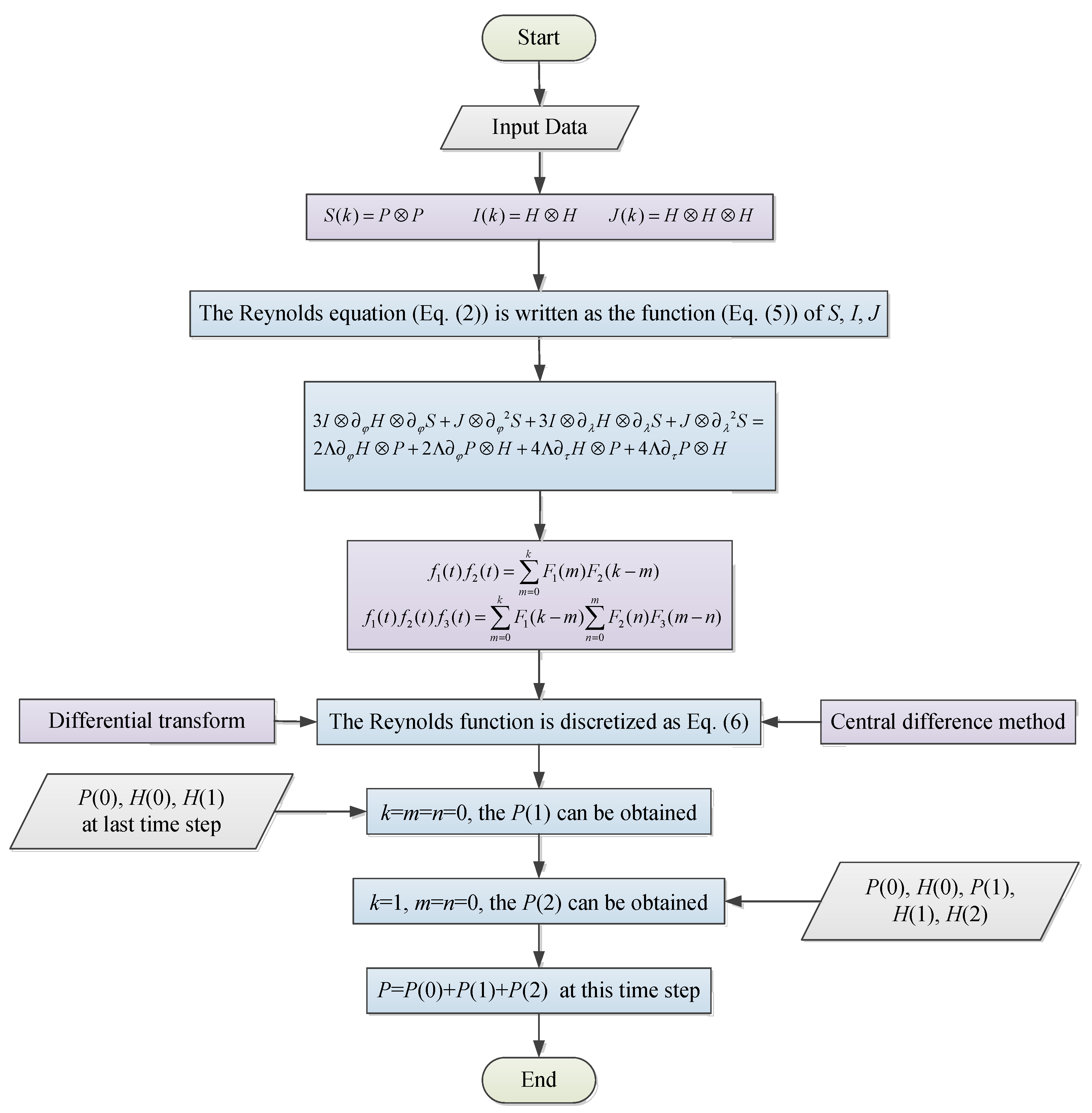
Figure 3.
The schematic drawing of the rod-fastened rotor system supported by two- and three-axial-groove gas bearings: (a) schematic drawing of the rod-fastened rotor; (b) the circumferential distribution of rods.
Figure 3.
The schematic drawing of the rod-fastened rotor system supported by two- and three-axial-groove gas bearings: (a) schematic drawing of the rod-fastened rotor; (b) the circumferential distribution of rods.

Figure 4.
Orbits comparison of the rod–fastened rotor and continuous integral rotor at ω = 1500 rad/s: (a) comparison of the orbits at ω = 1500 rad/s; (b) spectrogram of the continuous integral rotor at ω = 1500 rad/s.
Figure 4.
Orbits comparison of the rod–fastened rotor and continuous integral rotor at ω = 1500 rad/s: (a) comparison of the orbits at ω = 1500 rad/s; (b) spectrogram of the continuous integral rotor at ω = 1500 rad/s.

Figure 5.
Bifurcation diagram of the rod–fastened rotor at ω = 900~2500 rad/s.

Figure 6.
Quasiperiodic motion of the rod–fastened rotor at ω = 1000 rad/s: (a) orbit and Poincaré map at the left bearing station; (b) orbit and Poincaré map at the left disk station; (c) comparison of spectrogram at the left disk and left bearing stations; (d) comparison of the time series diagram at the left disk and left bearing stations.
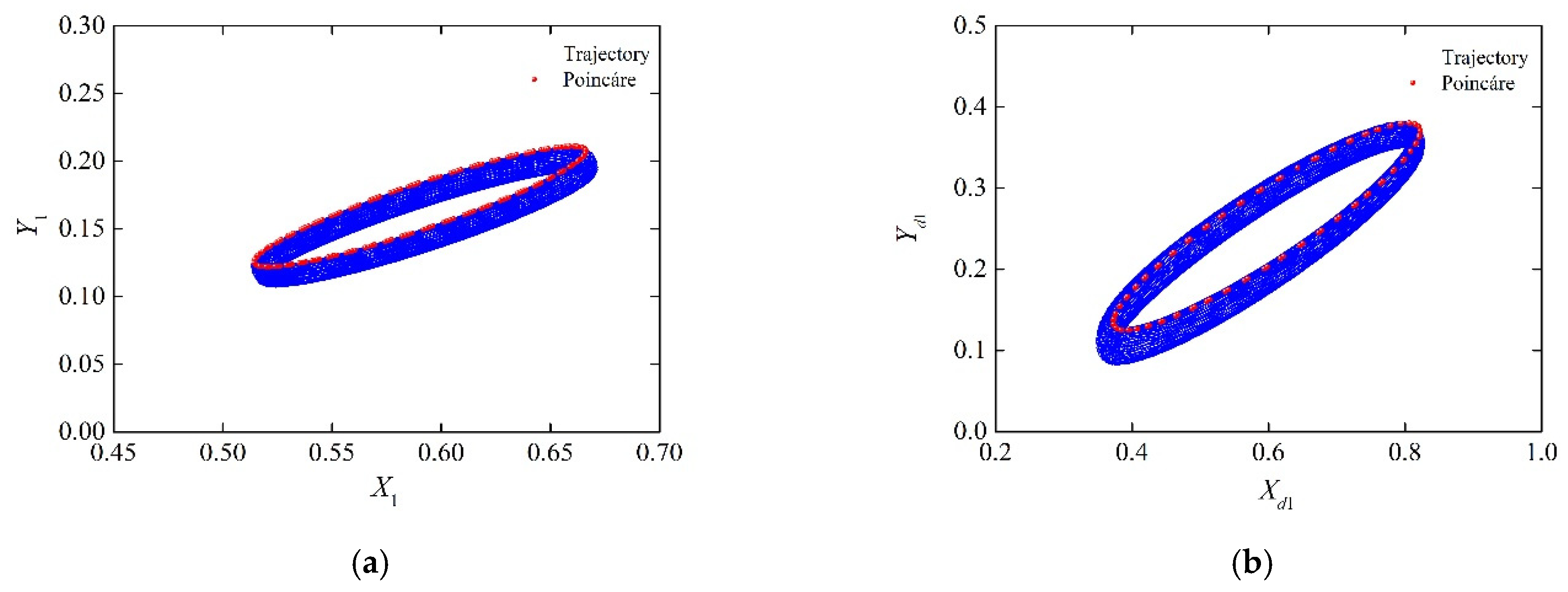

Figure 7.
Periodic motion of the rod–fastened rotor at ω = 1500 rad/s: (a) orbit and Poincaré map at the left bearing station; (b) orbit and Poincaré map at the left disk station; (c) comparison of spectrogram at the left disk and left bearing stations; (d) comparison of the time series diagram at the left disk and left bearing stations.
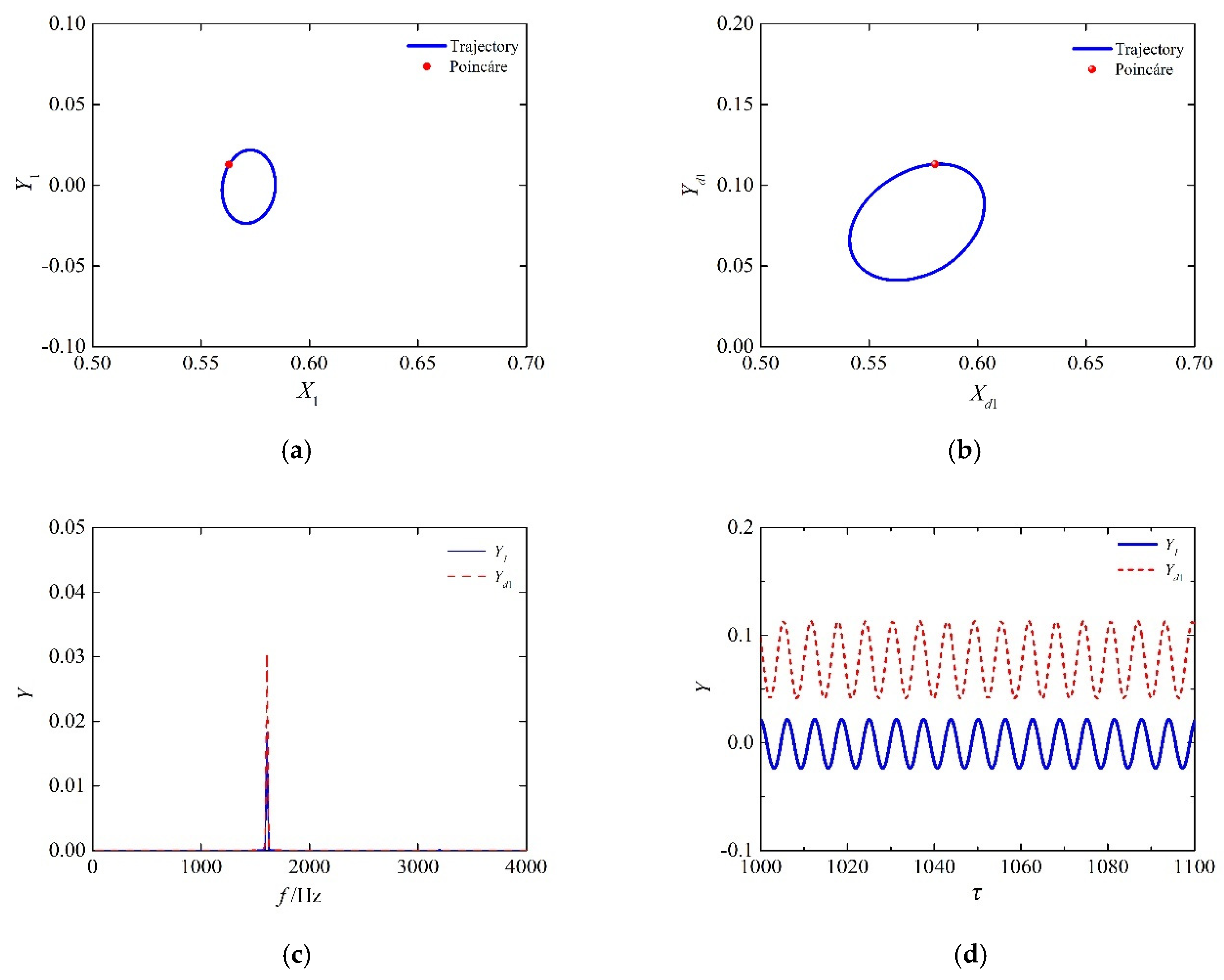
Figure 8.
Quasiperiodic motion of rod–fastened rotor at ω = 2000 rad/s: (a) orbit and Poincaré map at the left bearing station; (b) orbit and Poincaré map at the left disk station; (c) comparison of spectrogram at the left disk and left bearing stations; (d) comparison of the time series diagram at the left disk and left bearing stations.

Figure 9.
Quasiperiodic motion of the rod–fastened rotor at ω = 2500 rad/s: (a) orbit and Poincaré map at the left bearing station; (b) orbit and Poincaré map at the left disk station; (c) comparison of spectrogram at the left disk and left bearing stations; (d) comparison of the time series diagram at the left disk and left bearing stations.
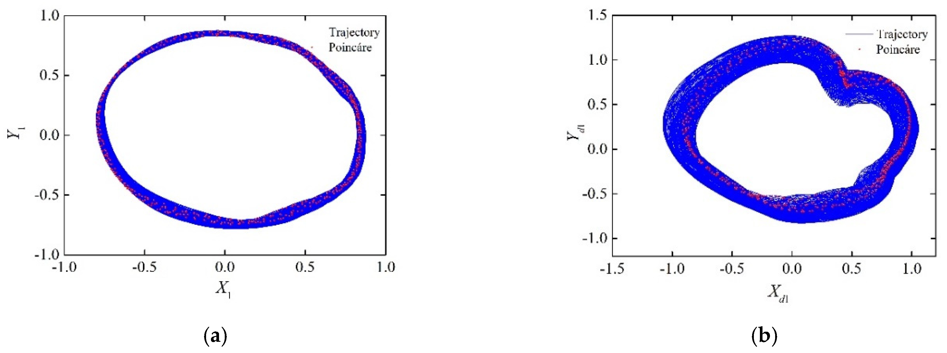

Figure 10.
When ω = 1500 rad/s, comparison of the rod–fastened rotor at α0 = 10° and 62.5°: (a) comparison of the orbits at the left bearing station; (b) comparison of the orbits at the left disk station.
Figure 10.
When ω = 1500 rad/s, comparison of the rod–fastened rotor at α0 = 10° and 62.5°: (a) comparison of the orbits at the left bearing station; (b) comparison of the orbits at the left disk station.

Figure 11.
When ω = 2000 rad/s, comparison of the rod–fastened rotor at α0 = 10° and 62.5°: (a) comparison of the orbits at the left bearing station; (b) comparison of the orbits at the left disk station.
Figure 11.
When ω = 2000 rad/s, comparison of the rod–fastened rotor at α0 = 10° and 62.5°: (a) comparison of the orbits at the left bearing station; (b) comparison of the orbits at the left disk station.
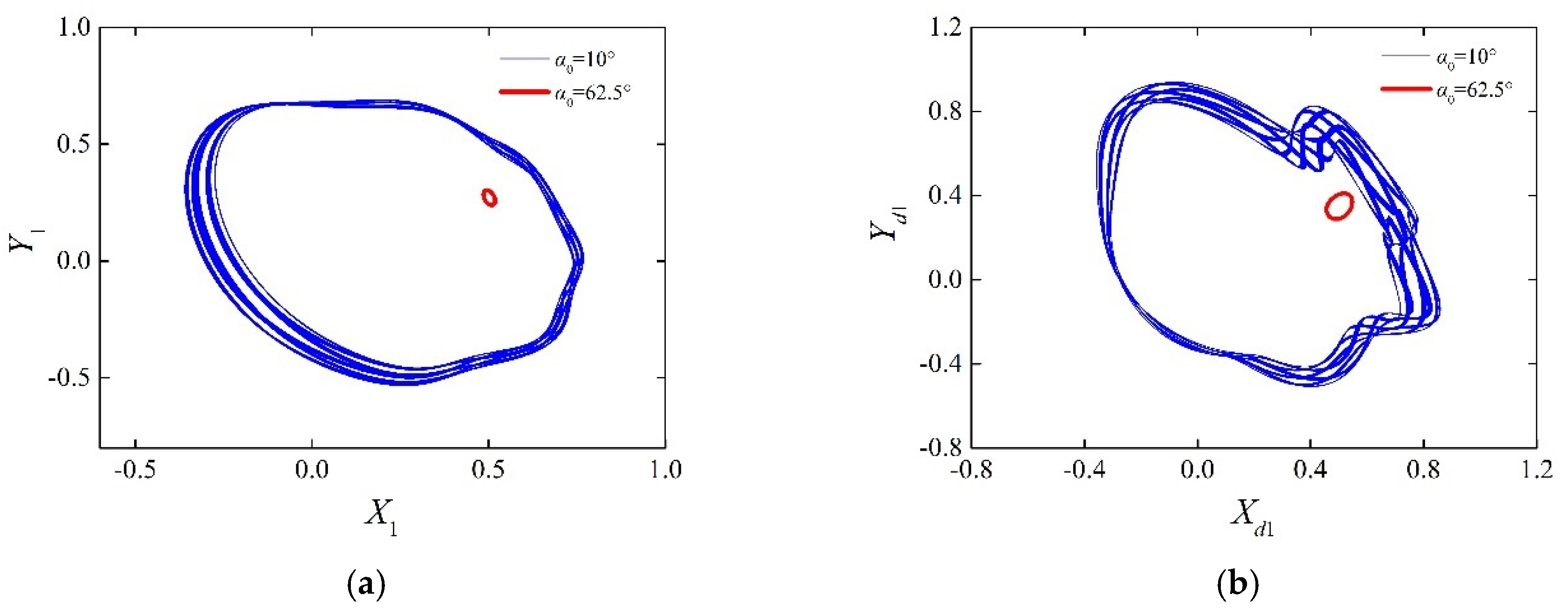
Figure 12.
When ω = 2500 rad/s, comparison of the rod–fastened rotor at α0 = 10°, 62.5°: (a) comparison of the orbits at the left bearing station; (b) comparison of the orbits at the left disk station.
Figure 12.
When ω = 2500 rad/s, comparison of the rod–fastened rotor at α0 = 10°, 62.5°: (a) comparison of the orbits at the left bearing station; (b) comparison of the orbits at the left disk station.

Figure 13.
When ω = 1500 rad/s, comparison of the rod–fastened rotors with 3-axial grooved and 2-axial grooved gas bearings: (a) comparison of the orbits at the left bearing station; (b) comparison of the orbits at the left disk station.
Figure 13.
When ω = 1500 rad/s, comparison of the rod–fastened rotors with 3-axial grooved and 2-axial grooved gas bearings: (a) comparison of the orbits at the left bearing station; (b) comparison of the orbits at the left disk station.

Figure 14.
When ω = 2000 rad/s, comparison of the rod–fastened rotors with 3-axial grooved and 2-axial grooved gas bearings, (a) comparison of the orbits at the left bearing station; (b) comparison of the orbits at the left disk station.
Figure 14.
When ω = 2000 rad/s, comparison of the rod–fastened rotors with 3-axial grooved and 2-axial grooved gas bearings, (a) comparison of the orbits at the left bearing station; (b) comparison of the orbits at the left disk station.


Table 1.
Integration constant parameters of Newmark-β method.
| Parameters | Value or Formula |
|---|---|
| α | 0.25 |
| δ, δ = 2α | 0.5 |
| a0 | 1/ατ2 |
| a1 | δ/ατ2 |
| a2 | 1/ατ |
| a3 | 1/2α − 1 |
| a4 | δ/α − 1 |
| a5 | (1/2α − 1) |
| a6 | (1 − δ)τ |
| a7 | δτ |
Table 2.
Structure parameter values of the rod-fastened rotor-gas bearing system.
| Parameter | Value | Unit |
|---|---|---|
| Structure parameters parameter values of the three-axial-groove gas bearing | ||
| Radius of bearing, Rb | 0.005 | m |
| Bearing width, Bb | 0.01 | m |
| Width-to-diameter ratio, Bb/2Rb | 1 | |
| Radial clearance, c | 5 × 10⁻⁶ | m |
| Position angle of pad, α0 | 10 | deg |
| Groove width angle, α | 5 | deg |
| Arc bushing angle, β | 115 | deg |
| Structure parameters parameter values of the rod-fastened rotor | ||
| Radius of shaft, R | 0.005 | m |
| Length of the left and right segments, l1 = l2 | 0.2 | m |
| Radius of disk, Rd | 0.01 | m |
| Width of disk, Bd | 0.02 | m |
| Mass eccentricities of the disk, ed1 = ed2 | 1 × 10⁻⁶ | m |
Publisher’s Note: MDPI stays neutral with regard to jurisdictional claims in published maps and institutional affiliations. |
© 2021 by the authors. Licensee MDPI, Basel, Switzerland. This article is an open access article distributed under the terms and conditions of the Creative Commons Attribution (CC BY) license (https://creativecommons.org/licenses/by/4.0/).
Share and Cite
MDPI and ACS Style
Li, S.; Lu, Y.; Zhang, Y.; Hei, D.; Zhao, X. Dynamics Investigation on Axial-Groove Gas Bearing-Rotor System with Rod-Fastened Structure. Appl. Sci. 2022, 12, 250. https://doi.org/10.3390/app12010250
AMA Style
Li S, Lu Y, Zhang Y, Hei D, Zhao X. Dynamics Investigation on Axial-Groove Gas Bearing-Rotor System with Rod-Fastened Structure. Applied Sciences. 2022; 12(1):250. https://doi.org/10.3390/app12010250
Chicago/Turabian StyleLi, Sha, Yanjun Lu, Yongfang Zhang, Di Hei, and Xiaowei Zhao. 2022. "Dynamics Investigation on Axial-Groove Gas Bearing-Rotor System with Rod-Fastened Structure" Applied Sciences 12, no. 1: 250. https://doi.org/10.3390/app12010250
Note that from the first issue of 2016, this journal uses article numbers instead of page numbers. See further details here.