
Energy Efficient, Highly Precise Cascade Dryness Control for Fibrous Tape by Induction-Based Surface Heating of a Rotating Steel Cylinder with Moving Inductors


Abstract
:1. Introduction
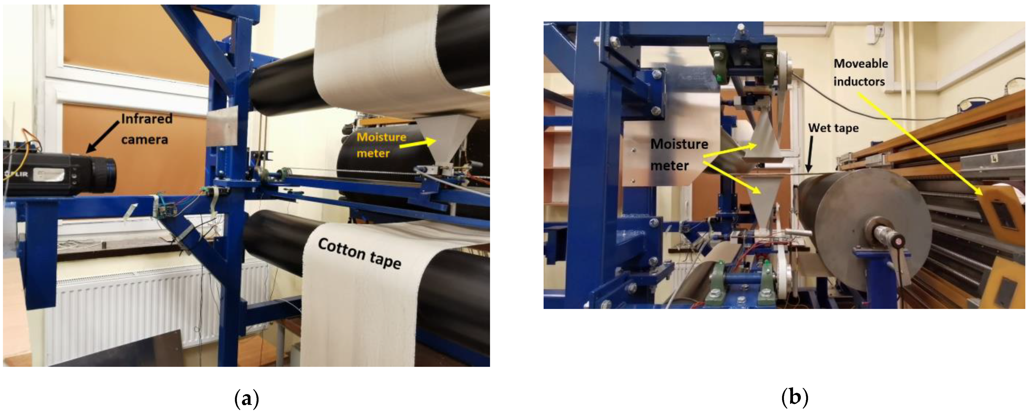
2. Experimental, Semi-Industrial Setup
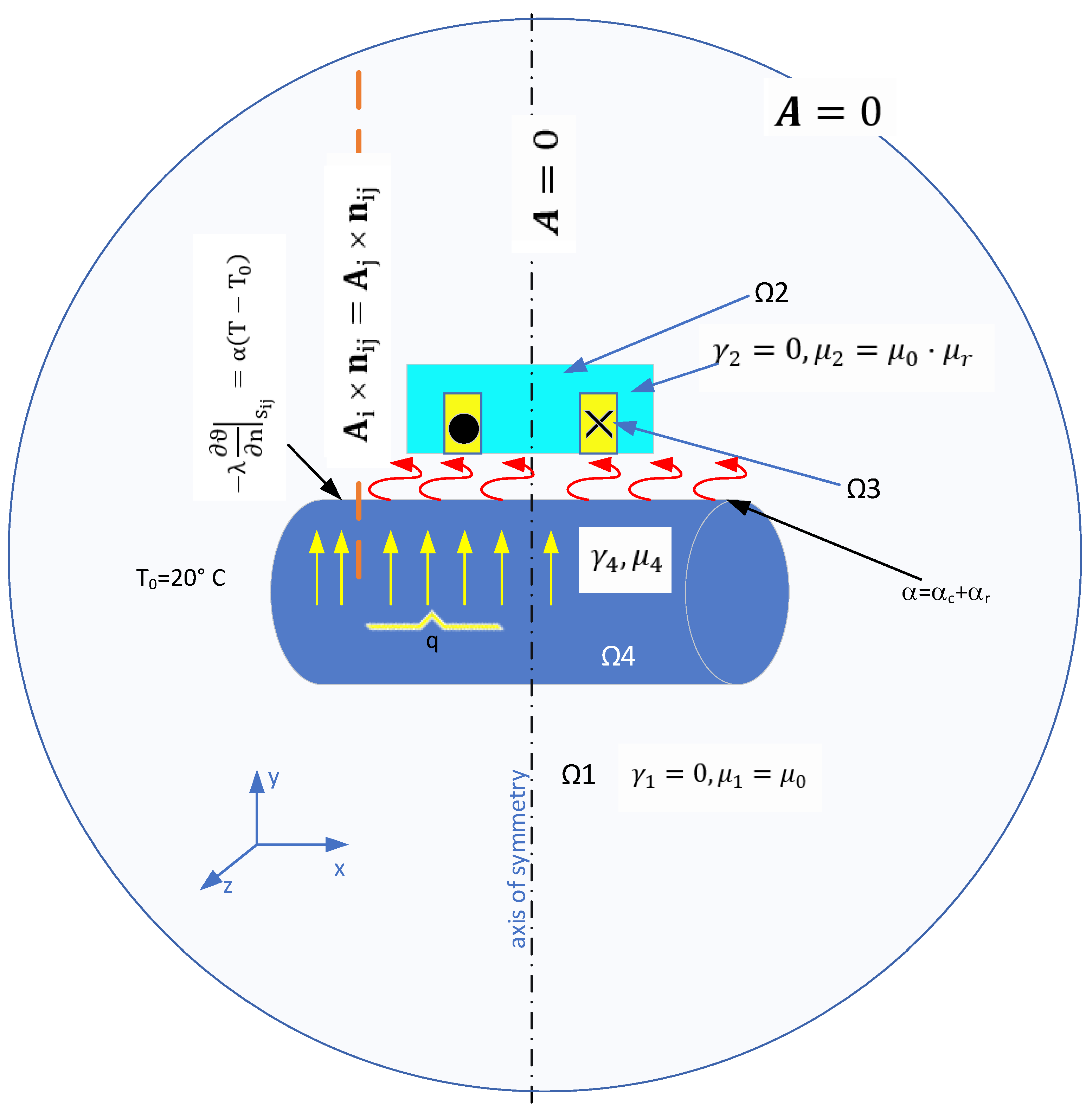
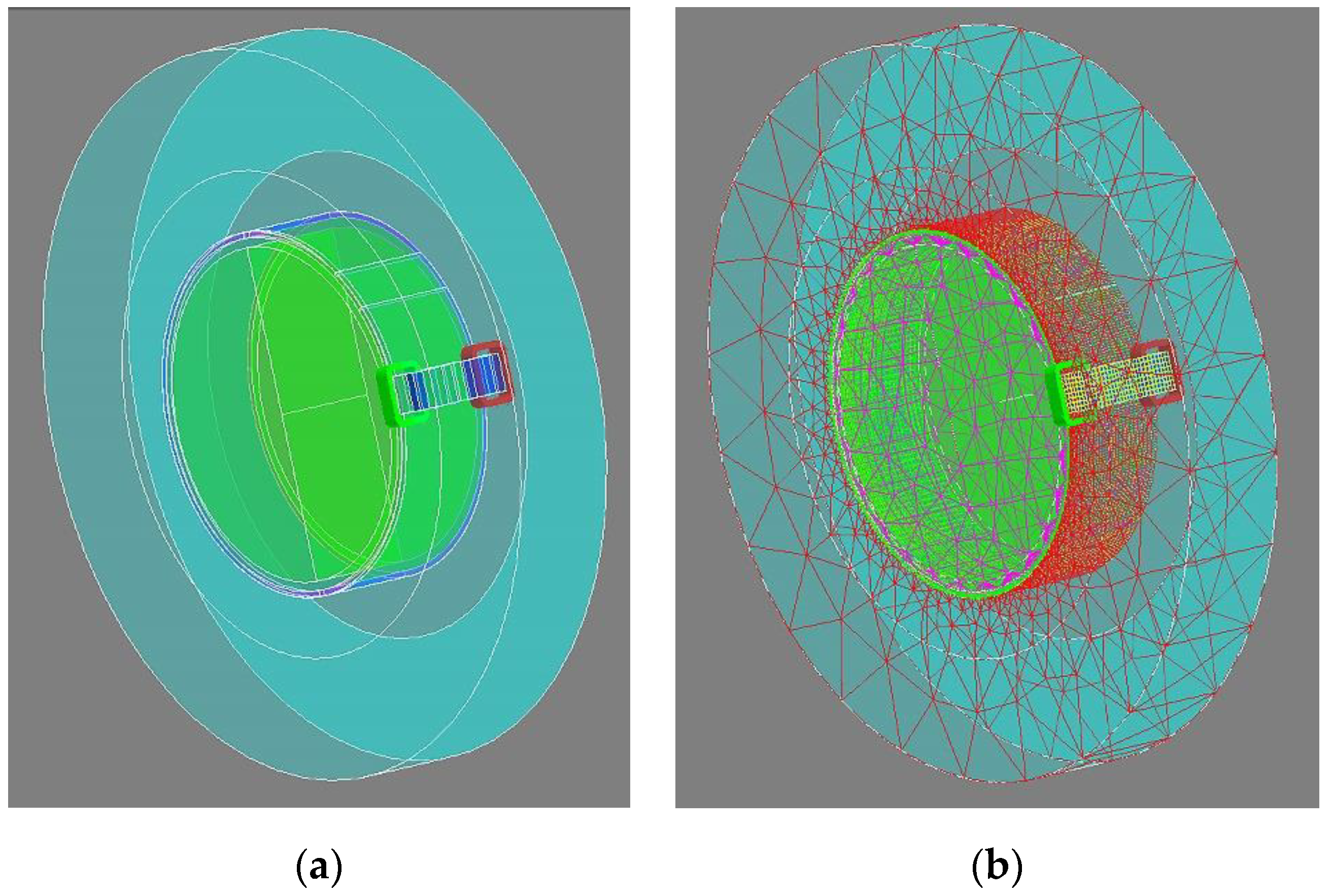
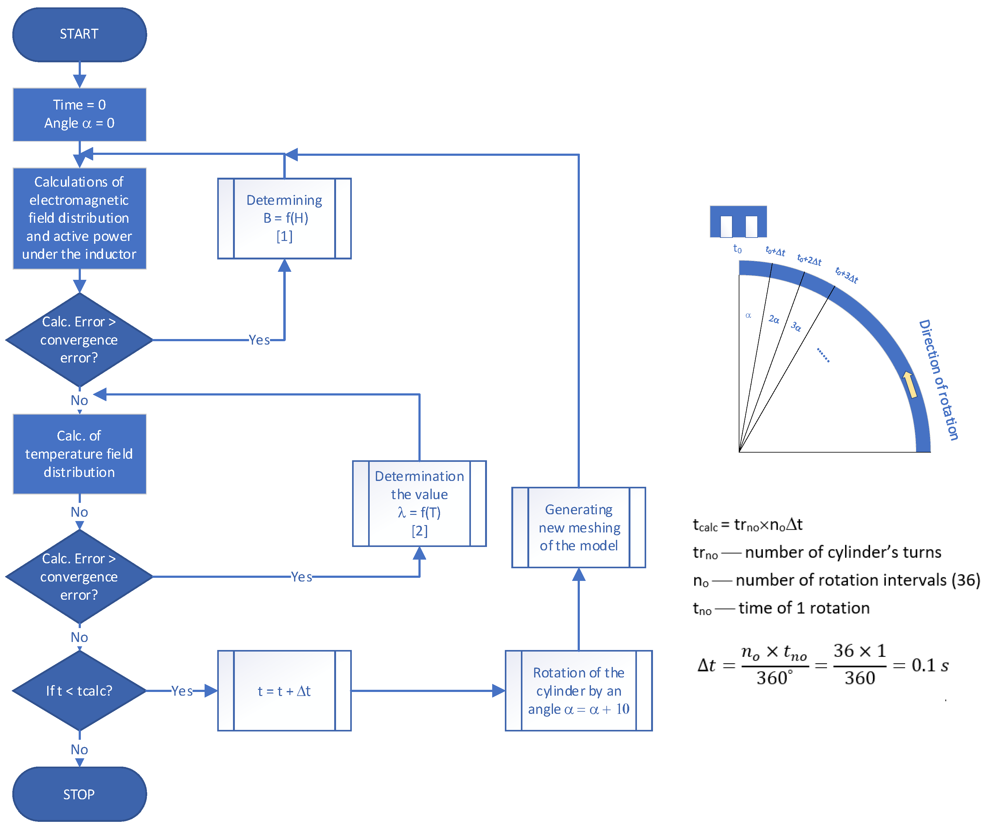
3. Numerical Model of Induction Heating a Rotating Steel Cylinder
- The anisotropy of the material properties of the cylinder area Ω4 was omitted. It was assumed that during calculation of the power P generated in the cylinder the cylinder does not move.
- In the winding area Ω3, a harmonic current of 17A flows in the entire volume of the winding (this is the so-called Litz wire). In this area, no active power is released.
- Zero conductivity of the ferromagnetic core Ω2 is assumed, and the anisotropy of the material properties of this area is omitted.
- For the area of the air gap and the environment of the heating system Ω1, a compromise is assumed between the size of the division into finite elements and the accuracy of the disappearance of the magnetic field at the edge of the area.
- In the induction heated rotating steel cylinder, the conduction current is much greater than the displacement current—i.e., γ ≫ ωε0εr.
- The induction of eddy currents in the cylinder due to its rotational speed is omitted.
- For the cylinder area Ω4:
- For magnetic shunt areas Ω2 and free space Ω1:
- For the inductor area Ω3:where Jw—the forced current density in the inductor winding; ω = 2πf—supply current pulsation (f—frequency); μ = μ0 μr—magnetic permeability of the medium (μ0 = 4μ∙10−7 H⁄m, μr—relative magnetic permeability of the medium); γ—conductivity of the medium; Jw—force current.
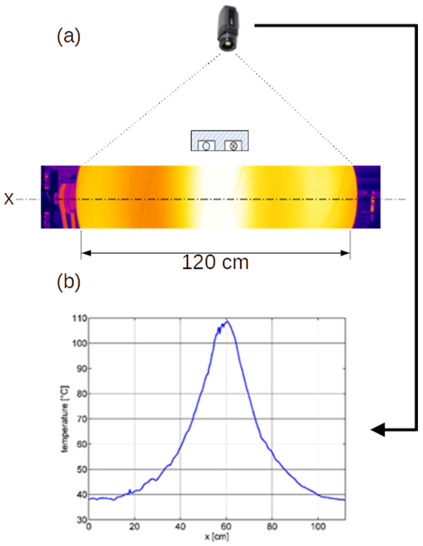
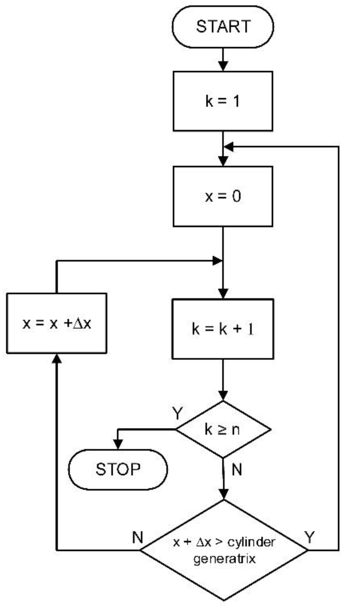
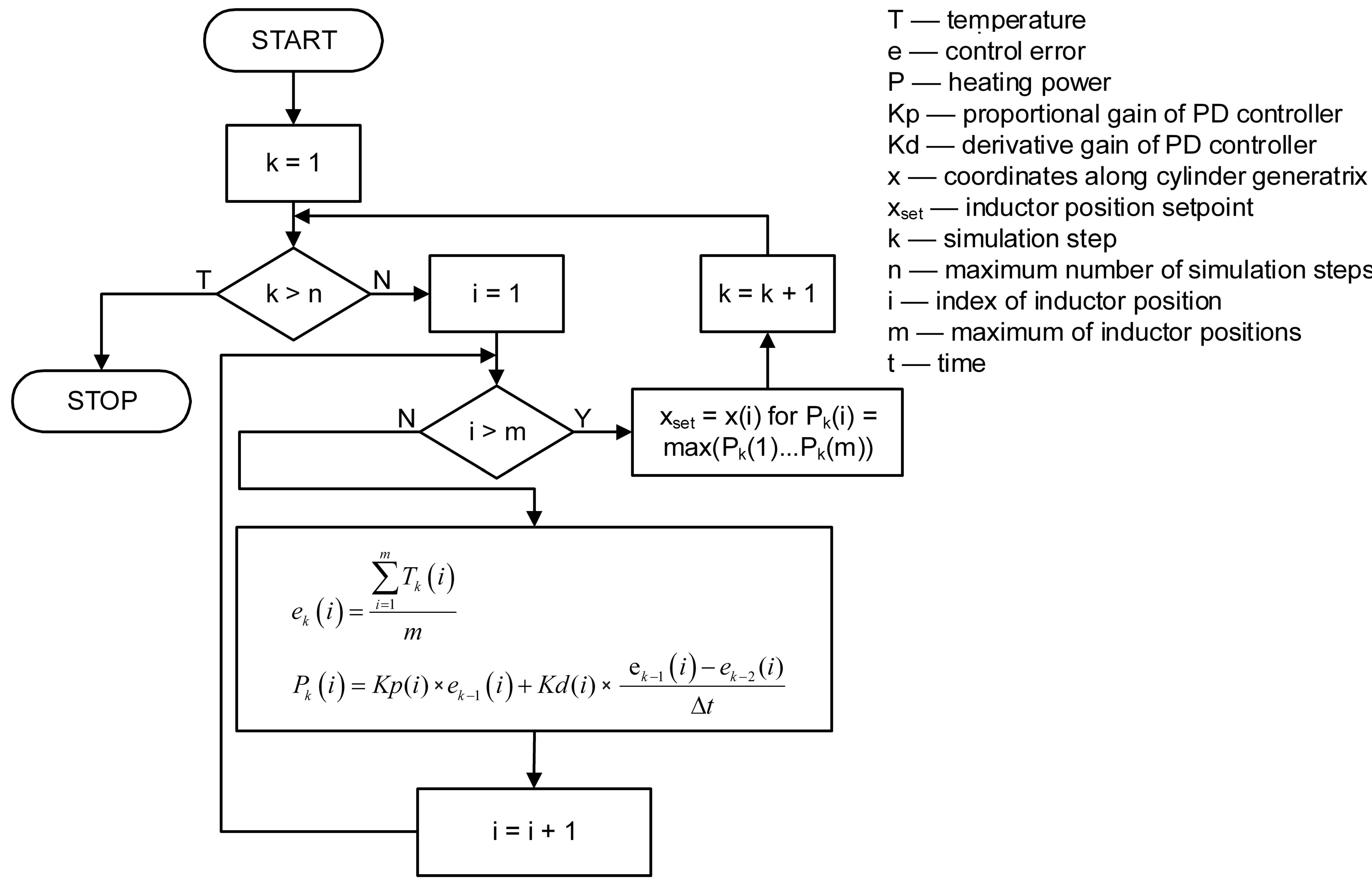
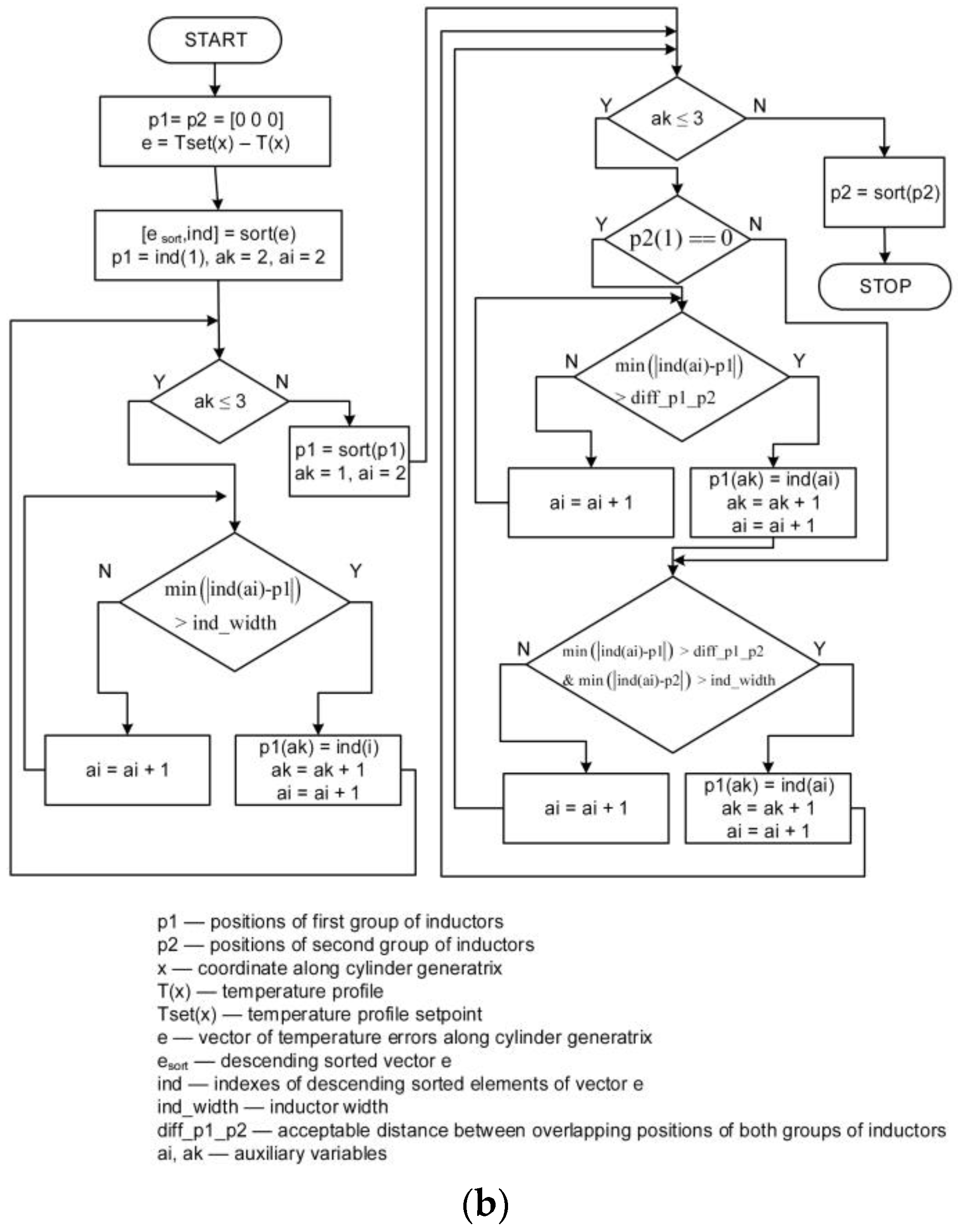
4. Temperature Profile Control
5. Dryness Control
6. Conclusions
Author Contributions
Funding
Institutional Review Board Statement
Informed Consent Statement
Data Availability Statement
Conflicts of Interest
References
- Chen, X.; Zheng, Q.; Dong, Y. Theoretical Estimation of Evaporation Heat in Paper Drying Process Based on Drying Curve. Processes 2021, 9, 1117. [Google Scholar] [CrossRef]
- Pavlík, Z.; Mihulka, J.; Fiala, L.; Černý, R. Application of Time-Domain Reflectometry for Measurement of Moisture Profiles in a Drying Experiment. Int. J. Thermophys. 2012, 33, 1661–1673. [Google Scholar] [CrossRef]
- Slätteke, O.; Åström, K.J. Modeling of a Steam Heated Rotating Cylinder—A Grey-Box Approach. In Proceedings of the American Control Conference, Portland, OR, USA, 8–10 June 2005; pp. 1449–1454. [Google Scholar]
- Ren, D.; Yao, J.; Wang, Y. Dryer Surface Temperature Control System Based on Improved Self-Adaptive Fuzzy Smith Prediction Controller; IEEE/IET Electronic Library (IEL): Piscataway, NJ, USA, 2005; pp. 1274–1279. [Google Scholar]
- Jang, J.-Y.; Chiu, Y.-W. Numerical and experimental thermal analysis for a metallic hollow cylinder subjected to step-wise electro-magnetic induction heating. Appl. Therm. Eng. 2007, 27, 1883–1894. [Google Scholar] [CrossRef]
- Demir, H. Experimental and numerical studies of natural convection from horizontal concreto cylinder heated with a cylindrical heat source. Int. Commun. Heat Mass Transf. 2010, 37, 422–429. [Google Scholar] [CrossRef]
- Kranjc, M.; Zupanic, A.; Miklavcic, D.; Jarm, T. Numerical analysis and thermographic investigation of induction heating. Int. J. Heat Mass Transf. 2010, 53, 3585–3591. [Google Scholar] [CrossRef]
- Clemens, M.; Gjonaj, E.; Pinder, P.; Weiland, T. Numerical Simulation of Coupled Transient Thermal and Electromagnetic Fields with the Finite Integration Method. IEEE Trans. Magn. 2000, 36, 1448–1452. [Google Scholar]
- Tsai, J.R.; Özisik, M.N. Transient, combined conduction and radiation in an absorbing, emitting, and isotropically scattering solid cylinder. J. Appl. Phys. 1988, 64, 3820–3824. [Google Scholar] [CrossRef]
- Barglik, J.; Smagór, A.; Smalcerz, A.; Desisa, D.G. Induction Heating of Gear Wheels in Consecutive Contour Hardening Process. Energies 2021, 14, 3885. [Google Scholar] [CrossRef]
- Zgraja, J. Simplified simulation technique of rotating, induction heated, calender rolls for study of temperature field control. Open Phys. 2018, 16, 326–331. [Google Scholar] [CrossRef] [Green Version]
- Rodriguez, G.; Vasseur, J.; Courtois, F. Design and Control of Drum Dryers for the Food Industry. Part 1. Set-Up of a Moisture Sensor and an Inductive Heater. J. Food Eng. 1996, 28, 271–282. [Google Scholar] [CrossRef]
- Kochan, O.; Kochan, R.; Bojko, O.; Chyrka, M. Temperature Measurement System Based on Thermocouple with Controlled Temperature Field. In Proceedings of the IEEE International Workshop on Intelligent Data Acquisition and Advanced Computing Systems: Technology and Applications, Dortmund, Germany, 6–8 September 2007; pp. 47–50. [Google Scholar]
- Li, F.; Ning, J.; Liang, S.Y. Analytical Modeling of the Temperature Using Uniform Moving Heat Source in Planar Induction Heating Process. Appl. Sci. 2019, 9, 1445. [Google Scholar] [CrossRef] [Green Version]
- Xie, Y.; Wang, Y. 3D temperature fi eld analysis of the induction motors with brokenbar fault. Appl. Therm. Eng. 2014, 66, 25–34. [Google Scholar] [CrossRef]
- Silver, D.; Salmon, R.; Barbieri, E.; Drakunov, S. Towards an Integrated Welding Testbed: Temperature Field Control. In Proceedings of the American Control Conference, Philadelphia, PA, USA, 24–26 June 1998; pp. 1023–1027. [Google Scholar]
- Chy, M.I.; Boulet, B. A New Method for Estimation and Control of Temperature Profile over a Sheet in Thermoforming Process. In Proceedings of the IEEE Industry Applications Society Annual Meeting, Houston, TX, USA, 3–7 October 2010; pp. 1–8. [Google Scholar]
- Girault, M.; Videcoq, E. Temperature regulation and tracking in a MIMO system with a mobile heat source by LQG control with a low order model. Control Eng. Pract. 2013, 21, 333–349. [Google Scholar] [CrossRef]
- Bougriou, C.; Bessaih, R.; Le Gall, R.; Solecki, J.C. Measurement of the temperature distribution on a circular plane fin by infrared thermography technique. Appl. Therm. Eng. 2004, 24, 813–825. [Google Scholar] [CrossRef]
- Guen, L.L.; Huchet, F.; Dumoulin, J.; Baudru, Y.; Tamagny, P. Convective heat transfer analysis in aggregates rotary drum reactor. Appl. Therm. Eng. 2013, 54, 131–139. [Google Scholar] [CrossRef]
- Datcu, S.; Ibos, L.; Candau, Y.; Mattei, S. Improvement of building wall surface temperature measurements by infrared thermography. Infrared Phys. Technol. 2005, 46, 451–467. [Google Scholar] [CrossRef]
- Cardone, G.; Ianiro, A.; dello Ioio, G.; Passaro, A. Temperature maps measurements on 3D surfaces with infrared thermography. Exp. Fluids 2012, 52, 375–385. [Google Scholar] [CrossRef]
- Johnson, M.A.; Moradi, M.H. PID Control. New Identification and Design Methods; Springer: London, UK, 2005; pp. 52–88. [Google Scholar]
- Wang, L. PID Control System Design and Automatic Tuning Using MATLAB/Simulink; Wiley-IEEE Press: Hoboken, NJ, USA, 2020; pp. 31–67. [Google Scholar]
- Matamoros, M.; Carlos, J.; Álvaro, G.B.; Sánchez, J.; Mancha, E.; Marcos, A.C.; Carrasco-Amador, J.P.; Pagador, J.B. Temperature and Humidity PID Controller for a Bioprinter Atmospheric Enclosure System. Micromachines 2020, 11, 999. [Google Scholar] [CrossRef]
- Xiong, S.; Wu, Z.; Li, W.; Li, D.; Zhang, T.; Lan, Y.; Zhang, X.; Ye, S.; Peng, S.; Han, Z.; et al. Improvement of Temperature and Humidity Control of Proton Exchange Membrane Fuel Cells. Sustainability 2021, 13, 10578. [Google Scholar] [CrossRef]
- Kochan, O.; Sapojnyk, H.; Kochan, R. Temperature Field Control Method Based on Neural Network. In Proceedings of the 7th IEEE International Conference on Intelligent Data Acquisition and Advanced Computing Systems: Technology and Applications, Berlin, Germany, 12–14 September 2013; pp. 21–24. [Google Scholar]
- Vasylkiv, N.; Kochan, O.; Kochan, R.; Chyrka, M. The Control System of the Profile of Temperature Field. In Proceedings of the IEEE International Workshop on Intelligent Data Acquisition and Advanced Computing Systems: Technology and Applications, Rende, Italy, 21–23 September 2009; pp. 201–206. [Google Scholar]
- Fraczyk, A.; Kucharski, J. Surface temperature control of a rotating cylinder heated by moving inductors. Appl. Therm. Eng. 2017, 125, 767–779. [Google Scholar] [CrossRef]
- Rodriguez, G.; Vasseur, J.; Courtois, F. Design and control of drum dryers for the food industry. Part 2. Automatic control. J. Food Eng. 1996, 30, 171–183. [Google Scholar] [CrossRef]
- Bai, X.; Zhang, H.; Wang, G. Modeling of the Moving Induction Heating Used as Secondary Heat Source in Weld-Based Additive Manufacturing; Springer: London, UK, 2014; pp. 717–727. [Google Scholar]
- Perez, S.; Thkrien, N.; Broadbent, A.D. Modelling the Continuous Drying of a Thin Sheet of Fibres on a Cylinder Heated by Electric Induction. Can. J. Chem. Eng. 2001, 79, 977–989. [Google Scholar] [CrossRef]
- Jianliang, S.; Shuo, L.; Chouwu, Q.; Yan, P. Numerical and experimental investigation of induction heating process of heavy cylinder. Appl. Therm. Eng. 2018, 134, 341–352. [Google Scholar]
- Shokouhmand, H.; Ghaffari, S. Thermal analysis of moving induction heating of a hollow cylinder with subsequent spray cooling: Effect of velocity, initial position of coil, and geometry. Appl. Math. Model. 2012, 36, 4304–4323. [Google Scholar] [CrossRef]
- Bermúdez, A.; Gómez, D.; Muñiz, M.C.; Salgado, P.; Vázquez, R. Numerical simulation of a thermo-electromagneto-hydrodynamic problem in an induction heating furnace. Appl. Numer. Math. 2009, 59, 2082–2104. [Google Scholar] [CrossRef]
- Rudnev, V. Unique Computer Modeling Approaches for Simulation of Induction Heating and Heat-Treating Processes. J. Mater. Eng. Perform. 2013, 22, 1899–1906. [Google Scholar] [CrossRef]
- Meyer, W.; Schilz, W.M. Feasibility Study of Density-Independent Moisture Measurement with Microwaves. IEEE Trans. Microw. Theory Tech. 1981, 29, 732–739. [Google Scholar] [CrossRef]
- Mikleš, J.; Fikar, M. Process Modelling, Identification, and Control; Springer: Berlin/Heidelberg, Germany, 2007; pp. 221–259. [Google Scholar]


| Symbol of Calculations Area | µr (−) | γ (S) | λ (W/m K) | ρc (J/m3 K) |
|---|---|---|---|---|
| Ω1 | 1 | 0 | - | - |
| Ω2 | 1000 | 0 | - | - |
| Ω3 | 1 | ∝ | - | - |
| Ω4 | According to B = f(H) charcteristics built in Flux software database (FLU_STEEL_1010_XC10) by Cedrat | 2.94 × 10⁶ | 47 | 4.5 × 10⁶ |
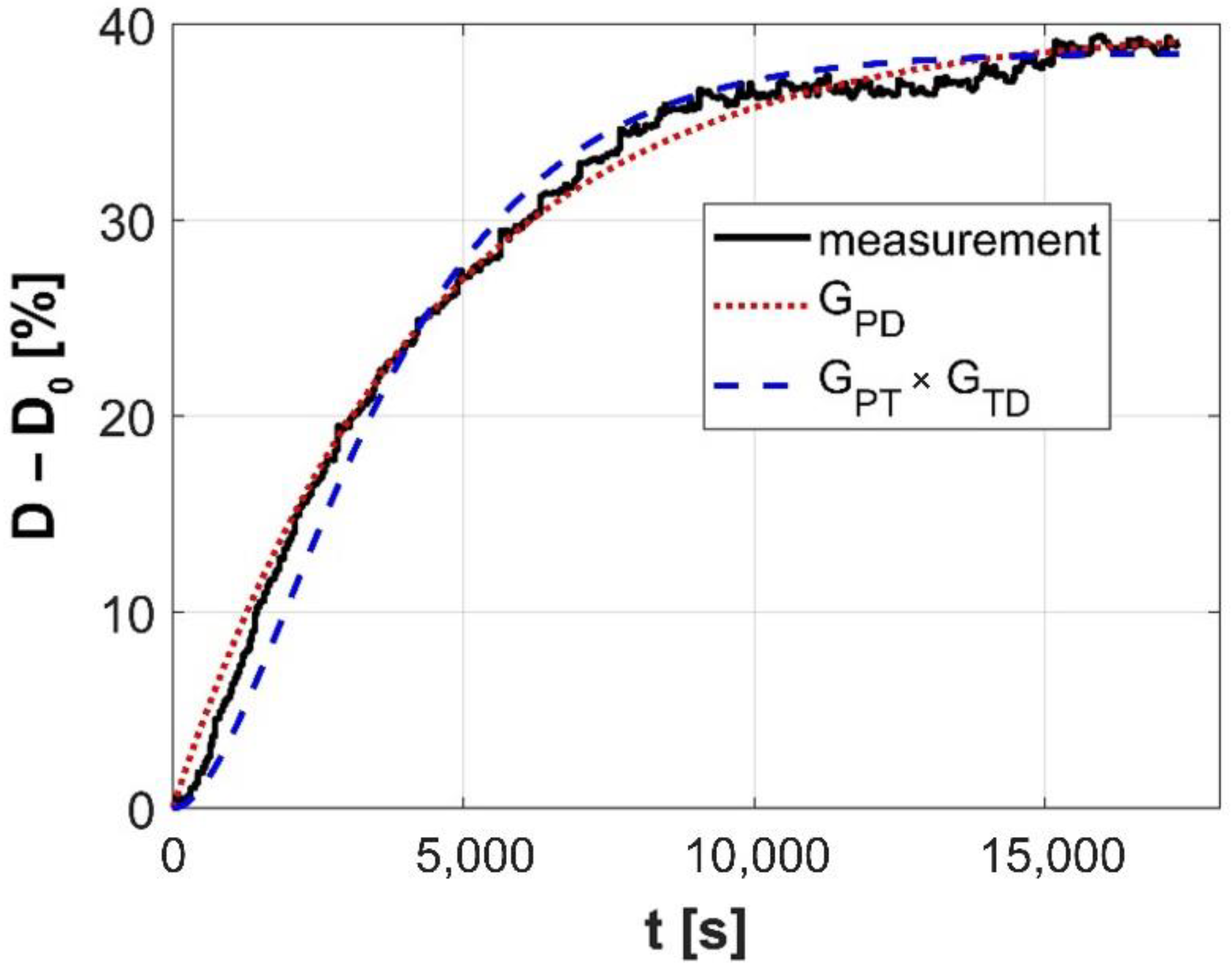
| GPD | GPT | GTD | |
|---|---|---|---|
| K | 3.99 × 10⁻² %/W | 1.48 × 10⁻² K/W | 2.61%/K |
| N | 4.42 × 10³ s | 2.05 × 10³ s | 1.87 × 10³ s |
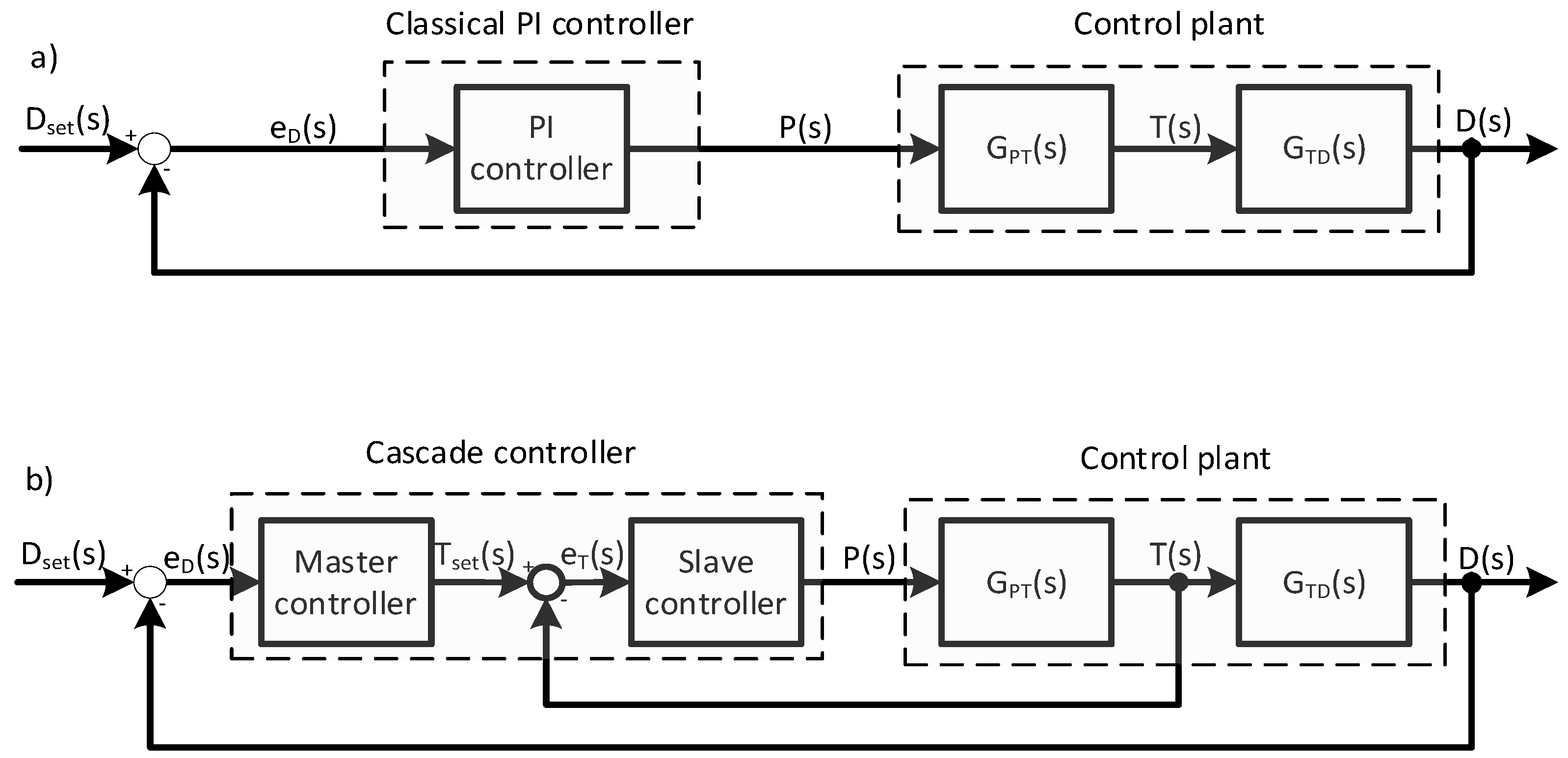
| PI Controller | Master Controller | Slave Controller | |
|---|---|---|---|
| Kp | 34.6 (W/%) | 0.75 (K/%) | 1064 (W/K) |
| Ki | 0.01 (W/%/s) | 4.2 × 10⁻⁴ (K/%/s) | 2.2 (W/K/s) |
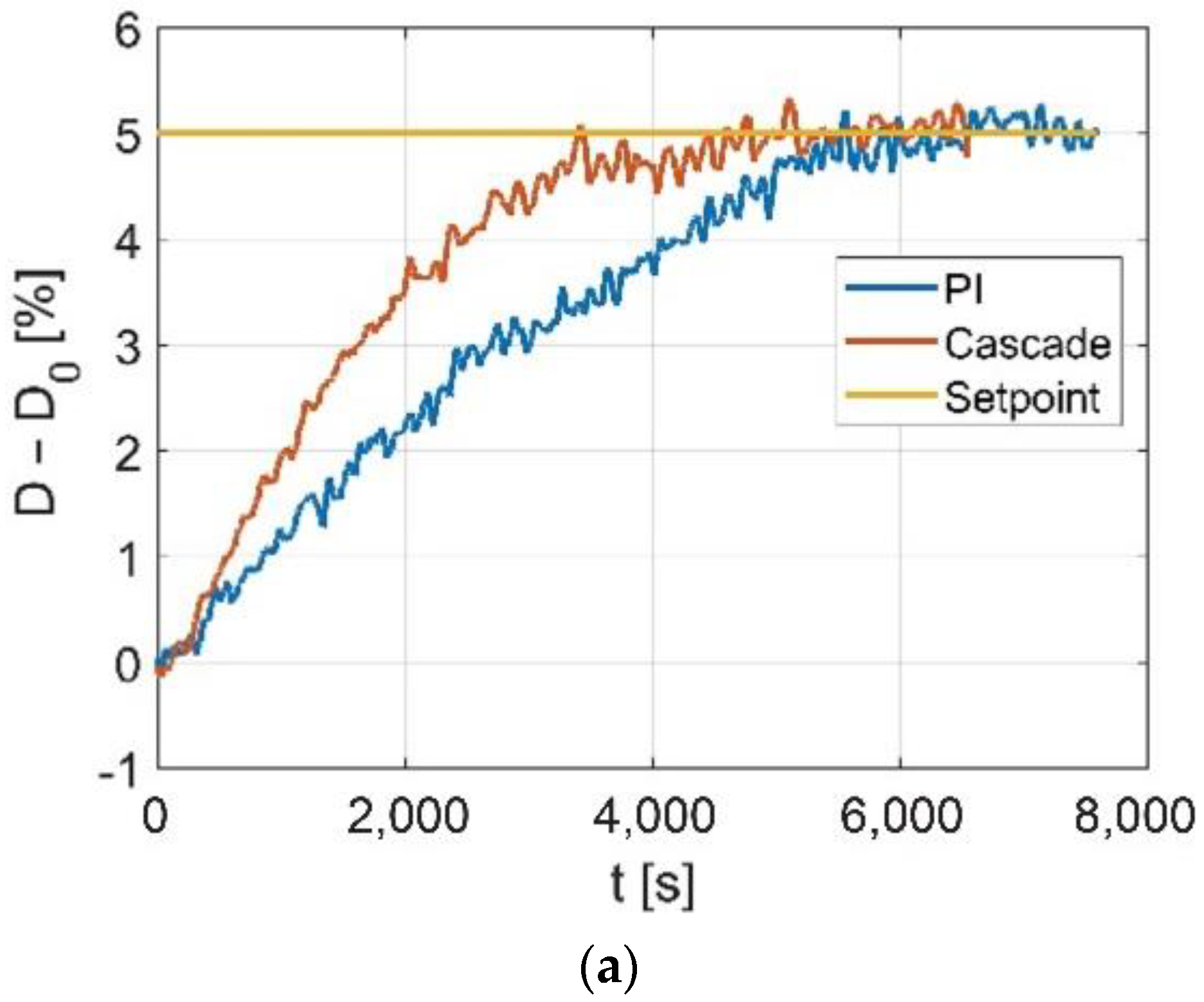
| Ts (s) | ITAE (% s) | |
|---|---|---|
| PI | 4972 | 2.24 × 10⁷ |
| Cascade | 3189 | 9.74 × 10⁶ |
Publisher’s Note: MDPI stays neutral with regard to jurisdictional claims in published maps and institutional affiliations. |
© 2021 by the authors. Licensee MDPI, Basel, Switzerland. This article is an open access article distributed under the terms and conditions of the Creative Commons Attribution (CC BY) license (https://creativecommons.org/licenses/by/4.0/).
Share and Cite
Kucharski, J.; Fraczyk, A.; Urbanek, P. Energy Efficient, Highly Precise Cascade Dryness Control for Fibrous Tape by Induction-Based Surface Heating of a Rotating Steel Cylinder with Moving Inductors. Appl. Sci. 2022, 12, 261. https://doi.org/10.3390/app12010261
Kucharski J, Fraczyk A, Urbanek P. Energy Efficient, Highly Precise Cascade Dryness Control for Fibrous Tape by Induction-Based Surface Heating of a Rotating Steel Cylinder with Moving Inductors. Applied Sciences. 2022; 12(1):261. https://doi.org/10.3390/app12010261
Chicago/Turabian StyleKucharski, Jacek, Andrzej Fraczyk, and Piotr Urbanek. 2022. "Energy Efficient, Highly Precise Cascade Dryness Control for Fibrous Tape by Induction-Based Surface Heating of a Rotating Steel Cylinder with Moving Inductors" Applied Sciences 12, no. 1: 261. https://doi.org/10.3390/app12010261