Abstract
This paper deals with the concept of multi-robot task allocation, referring to the assignment of multiple robots to tasks such that an objective function is maximized. The performance of existing meta-heuristic methods worsens as the number of robots or tasks increases. To tackle this problem, a novel Markov decision process formulation for multi-robot task allocation is presented for reinforcement learning. The proposed formulation sequentially allocates robots to tasks to minimize the total time taken to complete them. Additionally, we propose a deep reinforcement learning method to find the best allocation schedule for each problem. Our method adopts the cross-attention mechanism to compute the preference of robots to tasks. The experimental results show that the proposed method finds better solutions than meta-heuristic methods, especially when solving large-scale allocation problems.
1. Introduction
With the development of robot technology, the use of robots has increased in various fields such as automated factories, military weapons, autonomous vehicles, and drones. A robot can be controlled by an expert manually, but it is difficult to control a large number of robots simultaneously. If there are many robots, the job of an expert is then to determine the overall behavior of the robots, rather than controlling them individually. In such a case, the allocation of each robot can be done using an algorithms An example is illustrated by a situation involving ten rooms of different sizes in a building with five robot vacuum cleaners ready at the battery-charging machine. In this case, we want to allocate robots to rooms such that all rooms are cleaned and the total elapsed time is minimized. If we consider all possible allocations, there are possibilities that we have to consider for robots and permutations for ten rooms. This problem is an NP-hard problem, and finding an optimal solution takes a long time. This problem is termed the multi-robot task allocation (MRTA) problem, involving the assignment of tasks to multiple robots to achieve a given goal [1,2,3]. It is essential to assign tasks to robots efficiently for various applications of multi-robot systems, including reconnaissance [4,5], search and rescue [6,7], and transportation [8,9].
MRTA can be formulated as a problem of finding the optimal combination of a task schedule. Numerous approaches, including integer-linear programming (ILP) methods [6,10,11], auction-based approaches [12,13], and graph-based methods [14,15], have been suggested to solve such combinatorial optimization problems related to MRTA. However, they usually are not scalable to large-scale systems given that the number of possible combinations increases exponentially as the number of robots or tasks increases. In addition, they are not generalizable to complex problems without carefully handcrafted heuristics.
Recent advances in deep learning have led to a breakthrough in various fields of real-life applications including MRTA, aquaculture, thermal processes, energy system, mobile network, and vehicles [16,17,18,19,20,21,22]. The deep learning is applicable to various fields because of the high-dimensional representation that can encode complex knowledge in the real world. Vinyals et al. [21] and McClellan et al. [23] propose a deep-learning-based method for geometric problems applicable to the travelling salesman problem (TSP). The advantage of deep learning is that the features are learned end-to-end instead of using handcrafted features. Additionally, recent deep-learning-based methods outperform heuristic-based methods in various tasks. However, methods based on deep learning require a large amount of labeled data, and is hardly generalizable to out-of-distribution instances. Recently, Kool et al. [22] suggest a method based on reinforcement learning (RL) for combinatorial optimization problems including the TSP and vehicle routing problem (VRP). Unlike deep learning, RL-based methods interact with an environment to make decisions instead of learning from labeled data. For most of the real-world applications, acquiring the enough amount of labeled data is very expensive. Although existing deep-learning-based methods have shown promising results, they are limited to relatively simple problems, such as the TSP and VRP, which do not consider multi-task robots or multi-robot tasks.
Therefore, we propose an RL based MRTA method that can handle multi-robot tasks. Specifically, we focus on the allocation problems with single-task robots, multi-robot tasks, and time-extended assignments (ST-MR-TA). First, we formulate the problem as a Markov Decision Process (MDP) to adopt RL algorithms. Next, we suggest a hierarchical RL environment for MRTA, including an input representation and a reward function. Then, we propose an RL based MRTA method including a model structure and an optimization scheme. The dot-product cross-attention mechanism [24] is used in the model to guide the interactions between robots. Additionally, it provides the model with the interpretability in a sense that the attention weights indicate the importance of tasks to robots. The model is optimized with the policy gradient with greedy baseline [22], where the baseline is used to approximate the difficulty of each instance.
Our proposed method is evaluated in terms of the total time taken to complete the given tasks. We test our method in various settings with a different number of tasks. The results show that our method consistently outperforms the meta-heuristic baselines in different settings. Our method is not only superior in performance but also sample-efficient.
Our contributions are as follows: (1) an allocation algorithm in MDP formulation for complex scenarios that deal with multi-robot tasks, and (2) a deep RL based method for MRTA, including the model structure and the optimization scheme.
2. Background
2.1. Multi-Robot Task Allocation
MRTA is the problem of assigning robots to tasks while maximizing the given utility. This problem can be defined in various ways according to the environmental settings [2]. (1) the number of tasks that a robot can handle at one time, (2) the number of robots required for the task, and (3) the consideration of future planning. The first axis involves single-task robots (ST) and multi-task robots (MT). The second axis relates to single-robot tasks (SR) and multi-robot tasks (MR) and the last axis refers to instantaneous assignments (IA) and time-extended assignments (TA). The simplest combination is (ST-SR-IA) and the most complex combination is (MT-MR-TA). For multiple robots, the number of possible combinations increases exponentially as the number of robots increases. In addition, if the problem contains time-related assignments, it can be viewed as a decision process. In such a case, the problem is an -hard problem [1]. Although we can find a meta-heuristic algorithm to solve this type of problem, we must process the information of the environment to apply an algorithm in a simple manner, and loss of information will occur. For example, finding the shortest path algorithm in a village with the Dijkstra algorithm [25] requires a graph structure of the points, and it is difficult to consider the features of the streets. On the other hand, a neural network enables end-to-end training, and there is no loss of information when constructing the algorithm.
2.2. Reinforcement Learning
Recent advances in hardware have made deep learning possible, and an artificial neural network trained on massive amounts of data shows high performance in many fields, including vision and natural language processing. Reinforcement Learning (RL) has also progressed rapidly with deep learning. In RL, an agent learns the optimal action in a given state, and massive amounts of data and a simulator are required to train the agent. RL is defined on a Markov Decision Process with a tuple where is the set of all possible states and is a set of all possible actions. represents the transition probability, is the reward function and is a discount factor. The advantage of using MDP is that the decision process can be completely characterized by the current state. In other words, the current state is a sufficient statistic of the future. The goal of the training is to find the optimal policy which maximizes the expected discounted return of a state s where
Similarly, the goal of MRTA is to find the optimal policy which describes how to allocate agents. In detail, instantaneous allocation can be viewed as a type of RL with a discount factor of 0, meaning that the future is not considered. If time is related, MRTA problem includes the future impact, and then discount rate is a non-zero number. We hypothesize that the neural network can encode information optimal allocation.
There are several benefits of RL-based approaches. First, inference is fast despite the fact that training takes a long time. Inference computes the cross-attention between robots and tasks to allocate a single robot, with time complexity of . Because neural networks compress decision rules learned from the training data into parameters, it is possible to approximate the solution without considering all possible combinations. These trained parameters result in better performance than a meta-heuristic solution search. Next, this method can handle complex dependencies, where the optimal allocation for a task may be affected by the previous allocation. Additionally, it does not require delicately designed heuristics, which is one of the problems with meta-heuristic algorithms.
3. Problem Formulation
In this section, we describe a cooperative single task robots-multi robot tasks-time extended assignments (ST-MR-TA) problem. There are robots and tasks on a map. A robot moves to a task and works on it. When a robot works on a task, it reduces the workload by 1 at each time step, and the work is done when the workload is less than or equal to 0. Other agents can also undertake the work, and the workload of the task is reduced by n, with n representing the number of robots working on the task. We formulate this problem by means of (1) mixed integer programming and (2) a Markov decision process.
3.1. Mixed Integer Programming Formulation
In Equations (2)–(13), we describe the mixed integer programming (MIP) formulation of the cooperative ST-MR-TA problem following [26]. There are , a set of n tasks with x,y coordinates and workload for each task and , a set of m robots with x,y coordinates. We add initial task of workload 0 at coordinates (0,0) which is the initial location of robots. Additionally, robot can have battery constraint . The distance between two objects in the map is denoted by which is Euclidean distance. The variables are continuous variables represents start time and finish time of work on task by robot . The start time and finish time are 0 if robot is not allocated to task . The binary variable is 1 if task is assigned to robot and the binary variable is 1 if robot performs task followed by .
The constraints for the MIP formulation are described in Equations (2)–(13). Equation (2) is the objective of the problem. We add another variable which is greater than or equal to finish time and minimize it for all robots and tasks in Equation (3). Equations (4)–(6) are the domain of each variable. Equation (7) ensures the cumulative work time on task for all robots is larger than the workload of task . Equation (8) forces start time and finish time to be 0 if indexed task is not allocated to robot . The very large number M is used for the conditional trick. Equation (9) ensures that travel time of a successive task allocation is bounded by the distance of two allocated tasks. Equations (10) and (11) are used to match the allocation variable and the successive allocation variable . Equation (12) indicates the initial position for every robot . Equation (13) is optional for a battery constraint.
3.2. Markov Decision Process Formulation
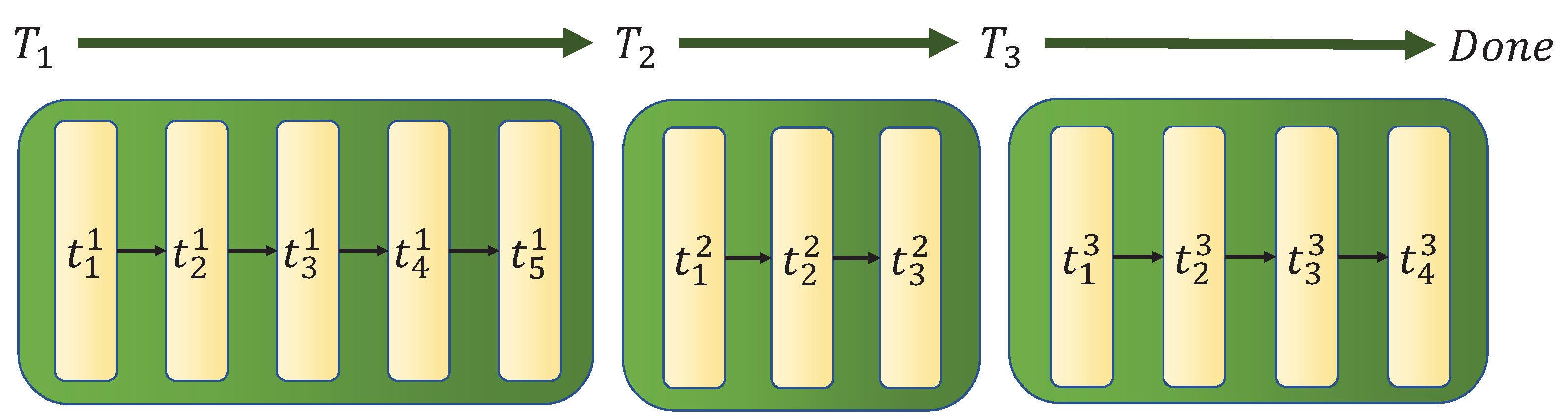
The cooperative ST-MR-TA problem can be solved by individual agents. That is, each robot chooses one of the remaining tasks. However, we can consider another option in which there is a manager responsible for robot allocation. Therefore, we suggest a MDP formulation in a hierarchical environment. This involves an outer environment whose action is only the allocation of idle robots to one of the remaining tasks and an inner environment which simulates robots and tasks. Both environments are designed as MDP, a sequence of state, action and reward [27]. An example of an episode in the hierarchical environment is described in Figure 1. We define as the total number of time steps spent in the inner environment, and the goal is to minimize .
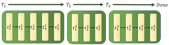
Figure 1.
Time steps of an example episode. The time step of the allocation environment is denoted by and the time step of the inner environment is denoted by . In this example, the allocation algorithm has allocated robots 3 times and is .
3.2.1. Allocation Environment
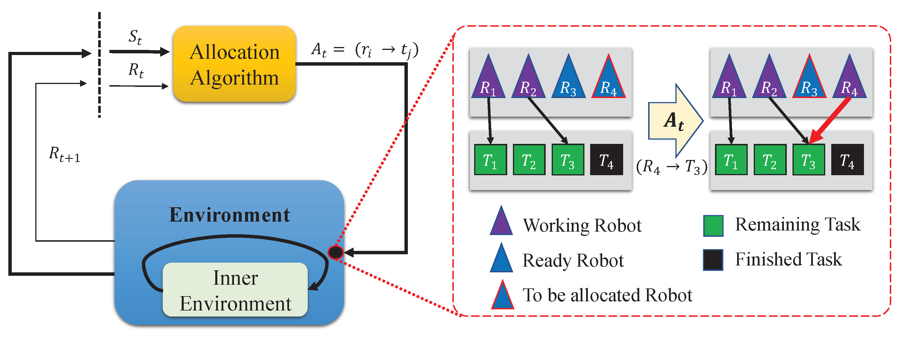
The role of the allocation environment is to allocate robot to task . We formulate the allocation environment as follows. The observation is the encoded information of n robots and the remaining tasks . The reward is a sparse reward with a penalty - at the end of an episode. The episode finishes when there are no remaining tasks.
We define as a set of remaining tasks whose workload is larger than 0, as a set of finished tasks and as a set of ready robots which are waiting to be allocated. A single time step of the environment is allocation of robot as described in Figure 2. Since we allocate only one robot in a single time step, it requires m successive environment time steps for the m ready robots. This successive allocation is denoted in the lines (4–6) in Algorithm 1. Therefore, the action is a mapping . Since a target task should be one of tasks in , we use the notation to describe the allocation of robot in Algorithm 1. Note that this environment is working independently from the real simulation of robots and is only responsible for the allocation of robots.
| Algorithm 1 Allocation Algorithm in MDP |
|

Figure 2.
A single time step of the allocation environment. When the allocation algorithm gives action to the environment, the environment gives the next state and reward pair . When we simulate the environment, robots choose actions in the inner environment which is also form of MDP. The allocation algorithm decides which task in is assigned to the given robot in . In this example, , , and the given robot is . The algorithm allocates the robot to task . After allocation, the inner environment runs until there is another ready robot. In this case, robot is another ready robot and next allocation happens immediately. Best viewed in color.
3.2.2. Inner Environment
The robots take one of actions (working or moving) in the inner environment. We first describe how to encode the information of the robots and tasks. Coordinates (, ) and (,) denote positions of robots and tasks. The state information of robot is one of ready, going and working. The state information of task is one of done and remaining. is the x,y coordinates of allocated task of robot . If there is no allocation of task to robot , . Since the problem is cooperative, there could be multiple robots working on and coming to the task . The allocation must consider the existence of robots on task , so that we can prevent unnecessary allocation (when the allocated task is done before reaching to the position) and encourage cooperation. Therefore we encode two types of information, and . is the number of working robots on task so that we can know when the task finishes. is a set of distances whose element is for robot coming to the task . We give mean and variance of distances coming to the task and 0 for each value if there is no robot coming to the task. The overall encoded information and are shown in Equations (15) and (16) for robots and tasks.
A single time step of the inner environment is 1 unit time behavior which means robot moves 1 unit distance when moving to task and reduces the workload by 1 when working on task . In the mathematical formulation of the problem, The start time and finish time are real values in MIP formulation. Therefore, the discrete environment does not match with the problem formulation. However, the two become more similar when the unit time approaches 0. By considering the gap between the formulation and the environment, we assume that the robot has reached the task when the distance of allocated task is less than some small positive value . When the robot reaches the task, we change the state of robot from moving to working. This change of state is described in line (11) in Algorithm 1. Even though the inner environment can be formulated by MDP, we do not train the robots because the goal of our paper is training task allocation method, not individual robots. The episode of the inner environment starts when there is no and runs until there are some robots who finished the assigned task. When a task is finished, the robots that worked on the task become idle and they are allocated to new tasks in . We designed this hierarchical architecture of environment for future study, where not only the outer MDP formulation is trained but also the robots are also trained.
4. Multi-Robot Task Allocation Methods
In this section, we describe our cross-attention mechanism-based method and baseline methods to allocate robots. We use baselines based on meta-heuristic algorithms proposed to solve combinatorial optimization problems. We test four algorithms, Random (RD), Stochastic Greedy (SG), Iterated Greedy (IG), and Genetic Algorithm (GA). Other meta-heuristic algorithms such as particle swarm optimization and ant colony optimization are also possible but not directly applicable to the MDP formulation.
4.1. Reinforcement Learning for MRTA
4.1.1. Model Structure
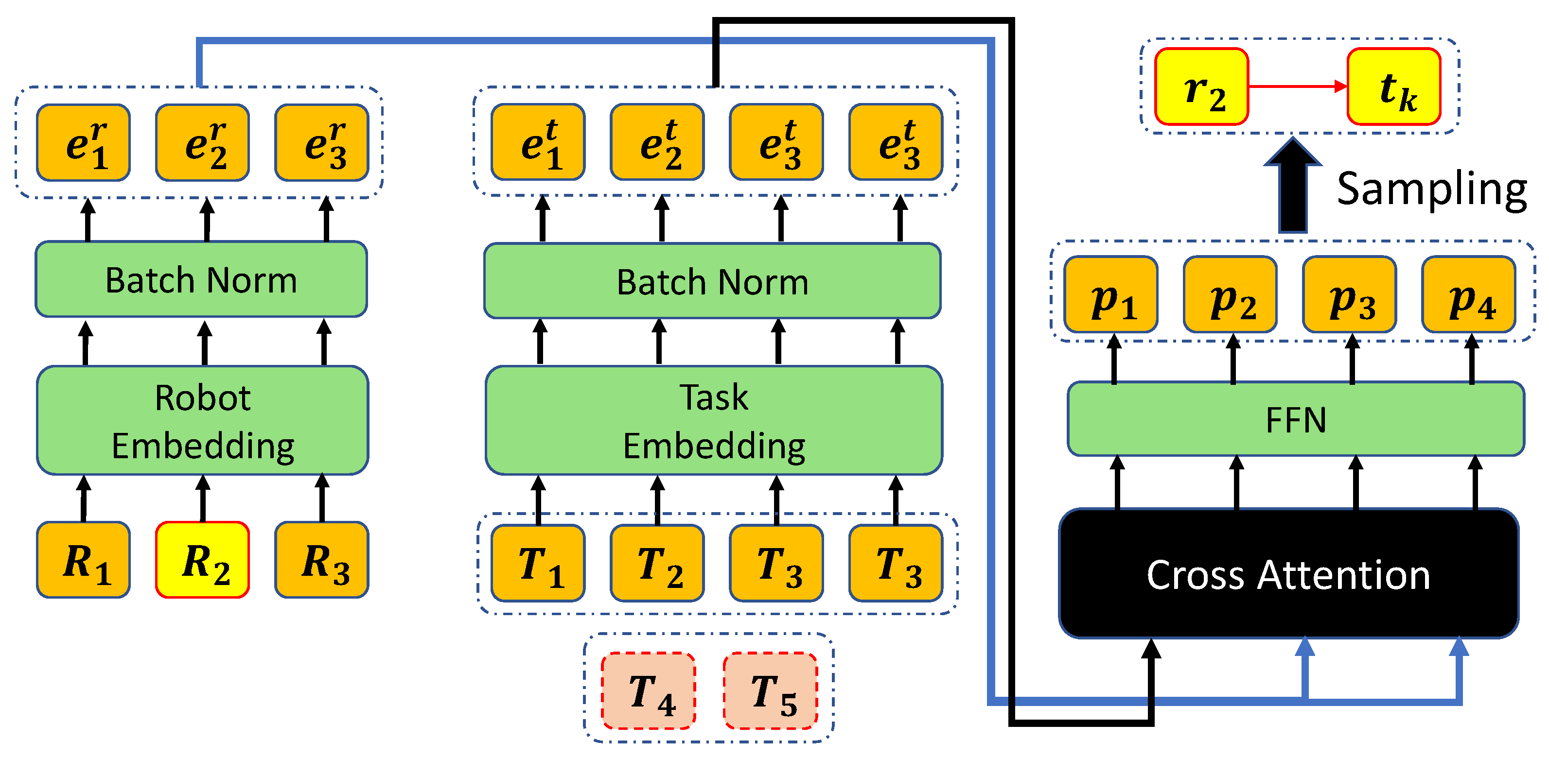
The deep learning model used in our method is based on the encoder and decoder architecture as described in Figure 3. The model is similar to the Transformer architecture by Vaswani et al. in [24]. The information of robots is embedded by the encoder using feed-forward neural network, ReLU activation, and batch normalization. Since our method allocates only one robot in a single time step, we must indicate the robot we are considering. Therefore, we use an additional one hot feature to indicate the robot and gets in Equation (17). Then is linearly projected to -dimensional vector through a linear projection with trainable parameters and .

Figure 3.
The neural network architecture for the MRTA. The robot to be allocated is and the remaining tasks are . Tasks are finished tasks and they are not used in the model. After normalizing the logits, we sample action from the probability. Here the robot is allocated to where . Best viewed in color.
Finally, we compute logit for each task embedding through linear projection with parameters and . Then we sample an index of the remaining task from the probabilities.
Figure 4 describes what is learned by the model. The model has two types of layers, (1) encoding layer for robots and tasks, and (2) cross-attention layer to compute the attention score between robots and tasks. The role of the encoding layer is to represent information of robots and tasks. The role of the cross-attention layer is to calculate an attention score which can be considered as an importance score between robots and tasks. This interpretability is an advantage of cross-attention layer compared to other types of layers. As a result, the neural network is trained to have better vector representation of robots and tasks and compute what is important. In addition, since the model is trained to find efficient allocation, the information for finding better allocation may be indirectly encoded in the neural network.
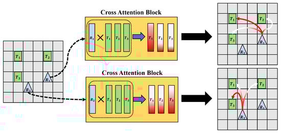
Figure 4.
What the model learns. The representation of robots and tasks includes the relationship information between robots and tasks. In this figure, is the most important task for the robot and is the most important task for the robot . The rectangle blocks in the cross-attention block are the vector representation of robot and task. The gradient on color denotes the importance of the task. More red is more important.
4.1.2. Optimization
We train the reinforcement learning model based on the policy gradient method with baseline. It is usual to use a critic network to estimate the value function. However, as noted in [22], using the baseline instead of a critic network is a better choice to solve combinatorial optimization. Therefore, we also construct baseline as the moving average of makespan while training. We also tried critic-network. However, training the value network made the training unstable. We optimized with Proximal Policy Optimizer (PPO) which clips the loss not to diverge. PPO takes the loss as the minimum value of the clipped advantage and the advantage:
We update the baseline after the end of the episode as the moving average of terminal reward which is .
The overall training algorithm of our model with baseline is in Algorithm 2.
| Algorithm 2:Policy Gradient with Surrogate Loss (full episode) |
|
4.2. Meta-Heuristics for MRTA
To evaluate the performance of the neural network, we compare with 3 types of meta-heuristic algorithms and a random selection. The solution of the cooperative MRTA problem can be viewed as permutations of n tasks for m robots. Then, the solution can be represented as Equation (22) where is j-th task by which robot visits. The size of the solution space is and exponentially increases as the number of tasks increases. Permutation-related solutions have already been dealt with meta-heuristics and we use variants following the construction of meta-heuristic algorithms in [28].
4.2.1. Genetic Algorithm
Genetic Algorithms (GA) are widely used to solve many optimization problems, including scheduling problems. The GA is a population-based algorithm that searches for the optimal solution from a set of candidates. When the population is given, the approach applies crossover and mutation to generate new children from the population. Then, it selects some of them and removes some of the original population so that a new population can be generated. However, our solution is the scheduling problem for m robots. Therefore we randomly choose robot in and find better solutions for the robot in a single iteration. In the scheduling problem, when the population of robot is given, and the crossover process randomly selects two solutions and task index k. Then, it switches the left side of the first solution and the right side of the second solution based on point k. This results in a new child, which is a combination of the original two solutions. If there are duplicated tasks, we use the original task of the parent. During the implementation, we pair all solutions in the population and undertake a crossover routine with a probability . The mutation randomly selects indexes of the two solutions in and switches the position of two tasks with probability . After applying two operations, the number of children is bounded by . During the selection, first we calculate the fitness of the children and choose the best P individuals from the candidates. The above process is repeated to achieve better solutions. We set P to 10 because setting P to a large number is computationally expensive.
4.2.2. Iterated Greedy Algorithm
Iterated Greedy (IG) is widely used to solve an optimization problem. Similar to GA, IG does not guarantee to find the optimal solution. However, the solution is improved over iteration through destruction, reconstruction, and local search. Unlike GA, IG is not a population-based algorithm and it starts from single solution . The algorithm randomly selects robot and improves the permutation . The deconstruction randomly selects d number of positions and removes them from the permutation and inserted them again into the deconstructed permutation in the reconstruction phase. The algorithm inserts the task using local search which considers all the possible positions and finds the position where the minimum makespan is achieved. It is guaranteed to finish all the tasks even though the permutation of robot is partial in the reconstruction phase because there are other robots whose permutation has all the tasks. The local search selects a random position of the permutation and considers all the possible positions to find the best position. We set d as length of the permutation.
4.2.3. Stochastic Greedy Algorithm
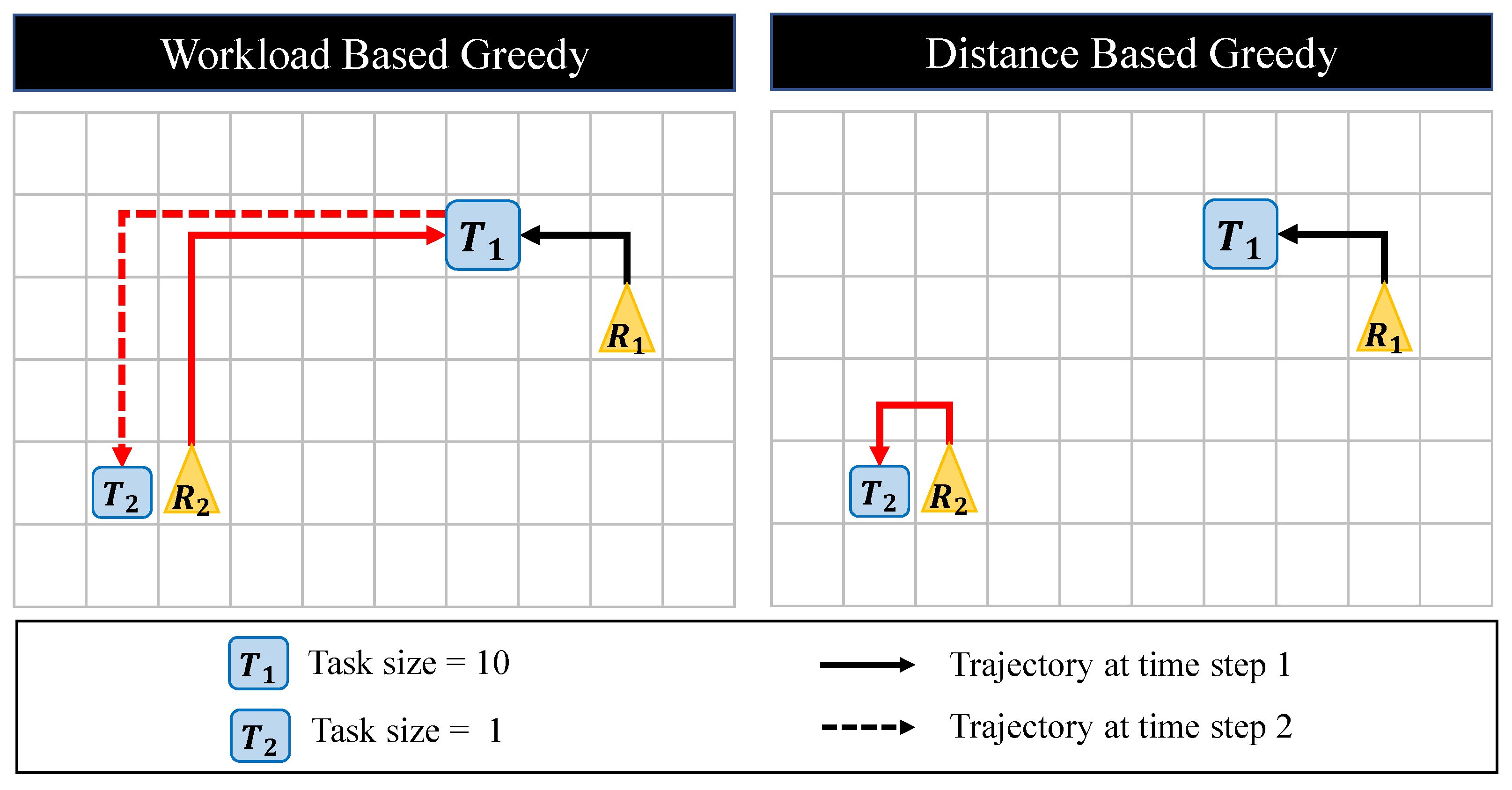
Simply selecting the closest task is one way to solve the problem. We can allocate robot to the nearest remaining task. However, there is one more factor to consider, the workload. Even when the work is close enough, in certain cases tasks at long distances must be considered first. On the other hand, there could be another problem instance in which working on the nearest task first is better than doing it later. Figure 5 shows such a case. Therefore we also considered a greedy algorithm as a baseline. Because the original greedy algorithm is deterministic, we modified the algorithm so that the allocation algorithm does not choose the nearest task, instead selecting one of the remaining tasks with a certain probability. In this work, we only considered distance-based greedy algorithm because the performance of the distance-based greedy algorithm was not good and we expect the same result with workload based greedy. Stochastic Greedy (SG) selects a task to be allocated to robot by sampling from the probability where N is normalization .
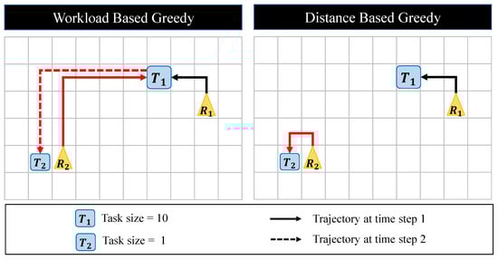
Figure 5.
Two types of greedy algorithm on an example problem. In workload based greedy, the robot chooses the task whose workload is larger than the workload of . In this case, the , while the makespan of the distance based greedy is . In this example, the travel time of at time step 1 is redundant in the workload based greedy.
4.2.4. Random Selection
In Random Selection, the algorithm randomly generates the permutation of tasks for all robots . There are two reasons why we use this methodology. In [22], it is noted that random sampling also works well in a simple combinatorial optimization problem. In addition, since our solution size is large (), the computation of a meta-heuristic algorithm could be a worse choice than sampling solutions. For example, local search in IG requires evaluation of near solutions and if the first solution is bad, the neighbor solutions are equally bad.
5. Experiments
5.1. Performance of Meta-Heuristic Algorithms
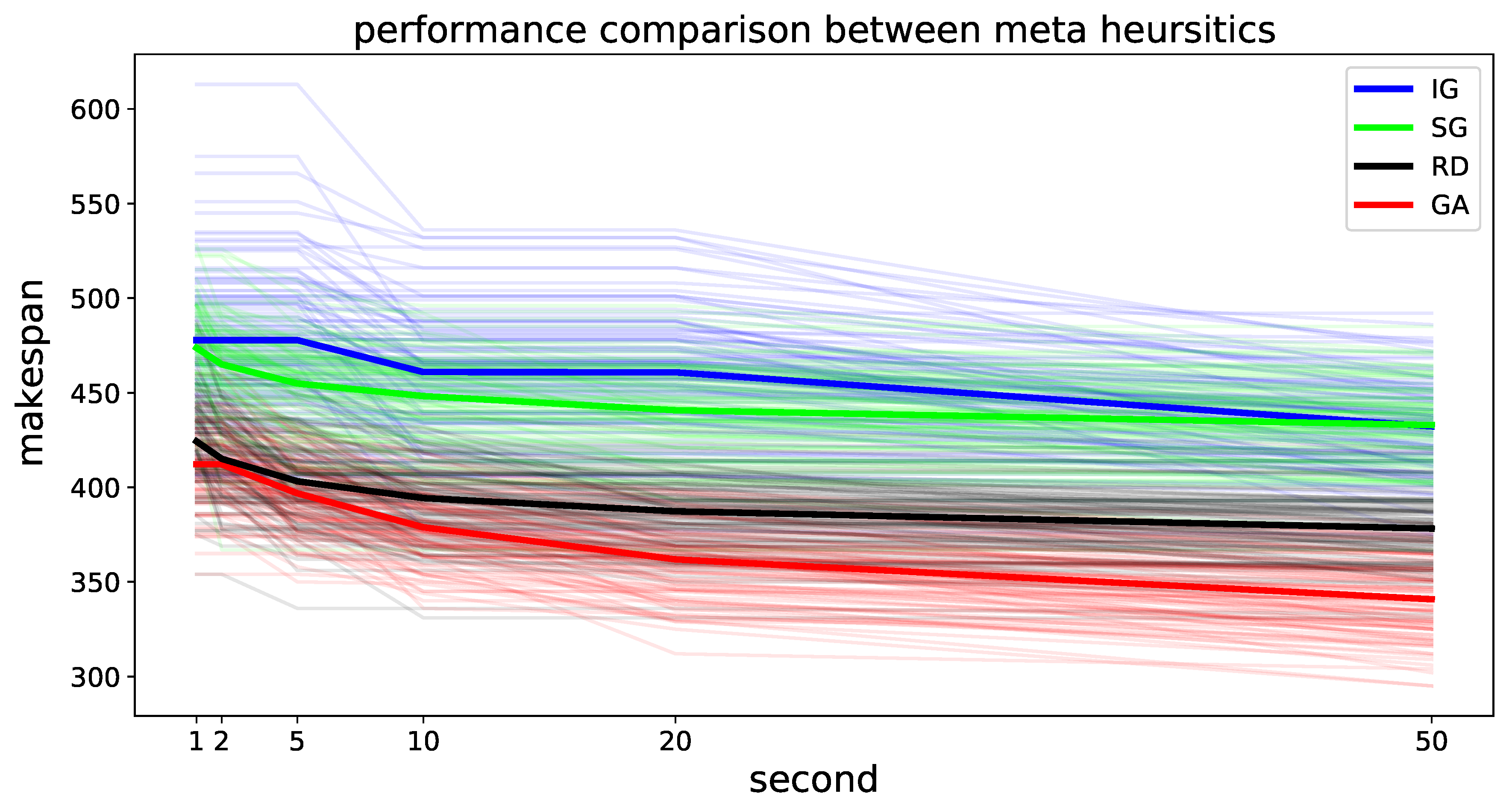
First, we demonstrate the performance of the Random, SG, IG, and GA algorithms on 100 samples. The makespan of the algorithms by time is shown in Figure 6. We find that the makespan of the meta-heuristic algorithm decreases. However, as noted in [22], the Random algorithm also works well considering the computation time. IG shows the worst performance because the most of the time is spent on the evaluation of the local search, and the performance does not increase significantly. GA shows the best performance among the four algorithms. This occurs because the population-based method can generate a variety of solutions by means of crossover and mutation from the best solution. The key parameters of the meta-heuristic algorithms were empirically determined. RD and SG require no parameters and IG requires a destruction parameter rate at which shows the best performance among four options . GA requires the crossover and mutation probabilities and the population size. We empirically found that population size N generated children of size and that evaluating all of these solutions was computationally expensive. Therefore we set the population size 10 which shows the most increasing performance among five options . All these parameters were tuned with problem instances with five robots and 50 tasks.

Figure 6.
Makespan for 4 algorithms in the environment with 5 robots and 30 tasks. The initial positions are random and workload is bounded by 20. We plot 100 sample results in light colors and the average in thick lines. The X-axis represents the real-time for 1, 2, 5, 10, 20, and 50 s. The lower the value, the better performance.
5.2. Reinforcement Learning
We test our model in five types of environments. We set the number of robots, the map size, and the workload to 5, 100, and 20, respectively. The tasks are randomly distributed in continuous 2D space and the initial workload for each robot is sampled uniformly in a set range . We tested 10, 20, 30, 40, and 50 tasks to compare the performances of thg algorithms on various difficulty levels. We trained IG, SG, RD, GA, and our model for 100 problem instances. All the problem instances are simulated separately using a single Intel(R) Xeon(R) Gold 6226 @ 2.70GHz CPU for meta-heuristics and RL-based model. RL-based model is optimized using NVIDIA Quadro RTX 6000 GPU. We trained the models for an hour and compared the minimum makespan. One of the most important hyperparameters of the deep learning model is the number of hidden dimensions. We add the experimental results with different numbers of hidden dimensions for 20 samples in Appendix A.2.
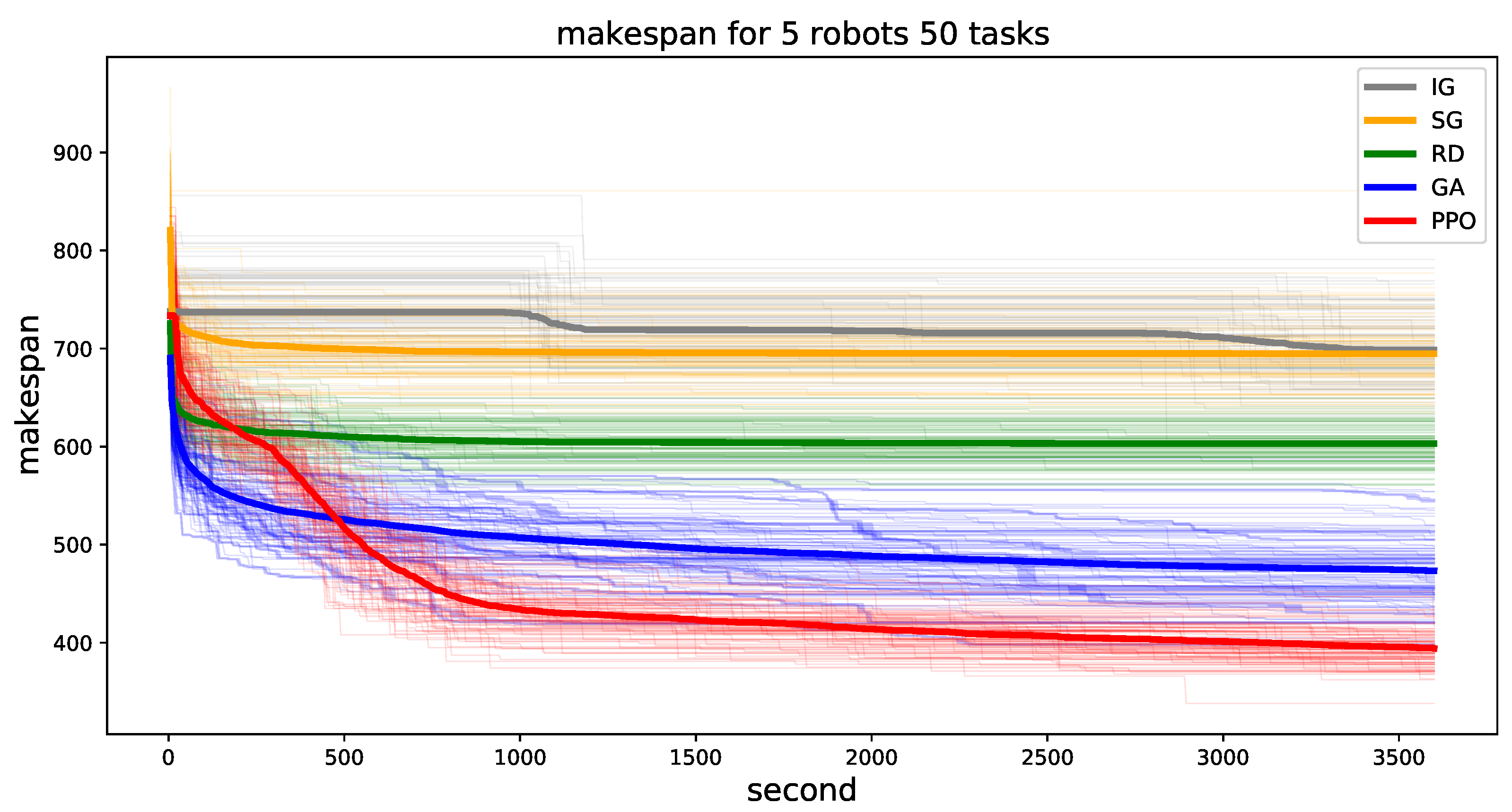
We plot the minimum makespan for 50 tasks in Figure 7. The other number of tasks can be found in Appendix A.1. In 50 tasks, IG, SG, and RD models converged early and the performance does not improve much, whereas the performance of GA improves over time. GA and RD find better solutions in the early steps than the RL-based search because we trained the model starting from random initialization, with time needed to train the initial weights. As training goes on, the proposed method (PPO-based) dominates the other models and the makespan decreases continuously. Unlike GA, whose makespan decreases mostly in the early phase (second < 500), the performance of our method improves smoothly and does not converge during the hour of training. Moreover, the variance of 100 samples is greater for GA than for our method. Therefore, we conclude that the solution search ability of our model improves over time and that it is not biased to a few problem instances. Although our model architecture (encoder-decoder) can be generalized to any number of robots and tasks, we do not pre-train the model, as the cooperative MRTA is more complex than TSP or VRP and because pre-training requires an additional training algorithm. We leave this as a future research project.
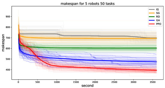
Figure 7.
Minimum makespan until the indexed time for 100 problem instances. The environment has 5 robots and 50 tasks. Thin lines indicate each instance problem and the bold lines indicate the average of all samples. Best viewed in color.
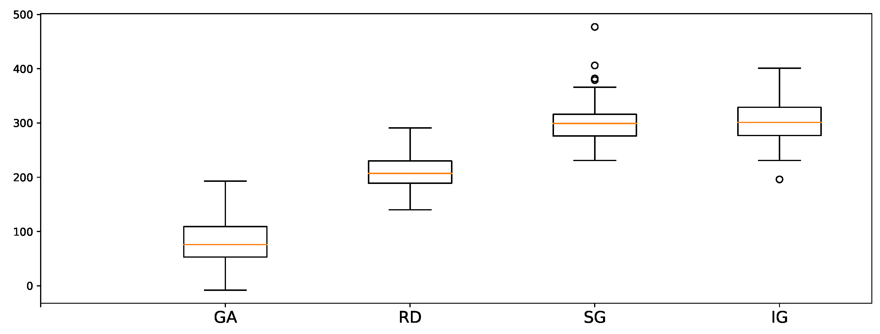
In Table 1, we present the minimal makespan found for 20, 40, and 60 min for all the models tested with the various number of tasks. As a result, GA performs the best among the meta-heuristic baselines (IG, SG and RD). In the case of 10 tasks, GA shows similar performance ( makespan) with our model ( makespan). In the case of 20 tasks, GA performs best at 20 min ( makespan), but our model shows better most of the time. When the number of tasks exceeds 30, our model shows significantly better performance than other models. As a result, we conclude that our model is highly effective for more complex problem. With regard to the statistical results, we compare two result groups, PPO and GA for 100 samples of 50 tasks. The p-value of two-sided T-test is which suggests that two samples have different average values. In addition, we measure the difference in performance for each sample, as shown in in Figure 8. This highlights the comparable performance in outcomes in a sample-wise manner. This difference in the makespan for each sample suggests that the proposed method finds better solutions than other meta-heuristics for all 100 samples.

Table 1.
Mean makespan of 100 problem instances for various number of tasks and allocation algorithms. The bold text indicates the best makespan among allocation algorithms.
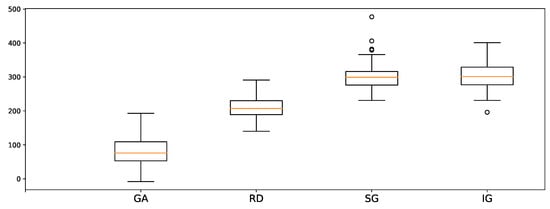
Figure 8.
Boxplot of the makespan gap between PPO and meta-heuristic methods for each 100 samples in 5 robots, 50 tasks, and 1 h training.
When the problem is simple (i.e., with ten tasks), GA outperforms our model. This occurs because the search space becomes smaller when the problem is simpler and because near-optimal solutions can be found with a random exhausted search. On the other hand, the on-policy method finds improved solutions based on the current solution. Therefore, the improved solution can be biased with regard to the initial policy, which is randomly initialized. Therefore, meta-heuristic-based methods perform relatively well in simpler problems. However, the performance difference (when the number of tasks is 10) is marginal and the proposed method significantly outperforms the baselines in more complex cases (when the number of tasks is larger).
We present the baseline reward and the on-policy reward while training. As shown in Figure 9, the baseline reward works as a lower bound for the on-policy reward, and the rates of increase for the two reward types are similar, as the improvement in the policy results in an improvement in the baseline and because the evaluation of the policy is based on the improved baseline.
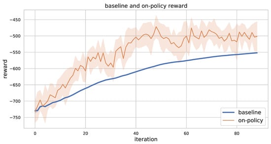
Figure 9.
On-policy reward and baseline reward for 5 robots and 50 tasks problem instance while training. We recorded all the simulated results and aggregated them by 5 episodes. The colored region represents confidence interval.
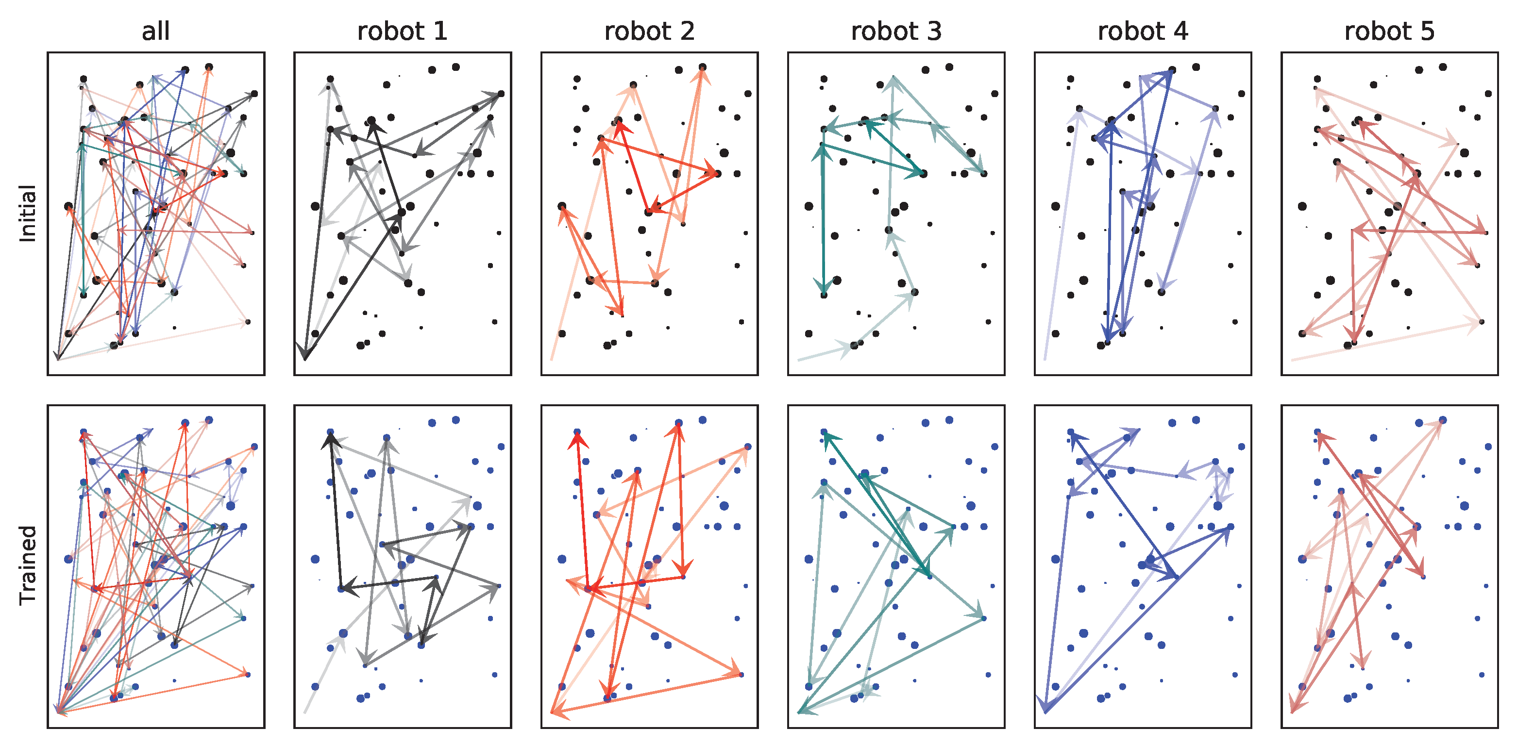
It is important to design an interpretable algorithm when devising a reliable autonomous allocation system. For example, the greedy algorithm selects tasks greedily and the overall plan is imaginable. However, the interpretation of the neural network is not intuitive even despite the fact that the RL based approach outperforms the baseline algorithms. We show a non-explainable property of our training scheme in Figure 10. We train a single instance of five robots and 50 tasks. There are no visual patterns that can be found despite the performance gain from the 658 makespan to 412 makespan. Although the RL-based algorithm shows a significant performance gain with the complex problems, it is still difficult to understand the intention of the neural network.
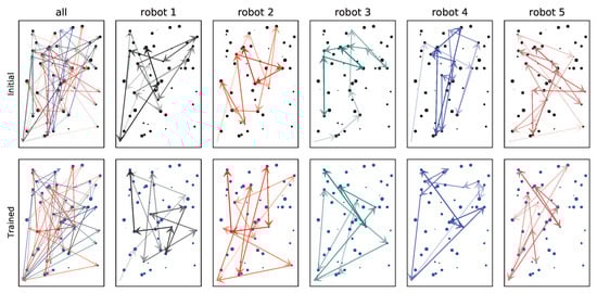
Figure 10.
The disadvantage of end-to-end training. The first row represents the initial allocation of the PPO model and the second row represents the trained model. The makespan before training is 658 while the trained allocation has 412 makespan. Even though the makespan is reduced by , the interpretation of the model is not trivial. The darker color represents the later allocation.
6. Conclusions
In this paper, we solve the cooperative ST-MR-TA problem, which is a more complex problem than other combinatorial problems. We propose the MDP formulation for this problem. Then, we suggest a robot and task cross-attention architecture to learn the allocation of robots to remaining tasks. We compare the deep RL-based method with several meta-heuristics and demonstrate a trade-off between the computation time and performance at various levels of complexity. Our method outperforms the baselines, especially when the problem is complex. The main limitation of our study is that the model decisions are not interpretable. Therefore, Explainable Artificial Intelligence in relation to MRTA problems can be suggested as a future research directions.
Author Contributions
Conceptualization, B.P., C.K. and J.C.; methodology, B.P., C.K.; software, B.P.; validation, C.K. and J.C.; formal analysis, B.P.; investigation, B.P., C.K.; resources, B.P., C.K. and J.C.; data curation, B.P.; writing—original draft preparation, B.P., C.K.; writing—review and editing, B.P., C.K. and J.C.; visualization, B.P.; supervision, J.C.; project administration, J.C.; funding acquisition, J.C. All authors have read and agreed to the published version of the manuscript.
Funding
This work has been supported by the Unmanned Swarm CPS Research Laboratory program of Defense Acquisition Program Administration and Agency for Defense Development (UD190029ED).
Data Availability Statement
All the problem instances are generated in python code with seed number 456. You can find the problem generator in https://github.com/fxnnxc/cooperative_mrta_problem_generator (accessed on 24 December 2021).
Conflicts of Interest
The authors declare no conflict of interest.
Appendix A
Appendix A.1. Training Results on Various Number of Tasks
The ability to find a better solution depends on the complexity of problem. For detailed comparison between RL-based approach and meta-heurstics, we plot the solution search progress for 10, 20, 30 and 40 number of tasks in Figure A1. As the problem becomes more difficult, RL based solution search outperforms other baselines.
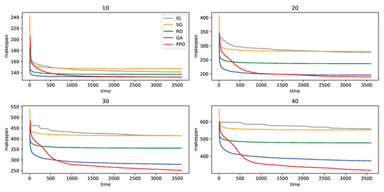
Figure A1.
Minimum makespan until the indexed time for 100 problem instances of 5 robots and various number of tasks. The title of each graph is the number of tasks. The lines indicate the average of all samples for each model.
Figure A1.
Minimum makespan until the indexed time for 100 problem instances of 5 robots and various number of tasks. The title of each graph is the number of tasks. The lines indicate the average of all samples for each model.
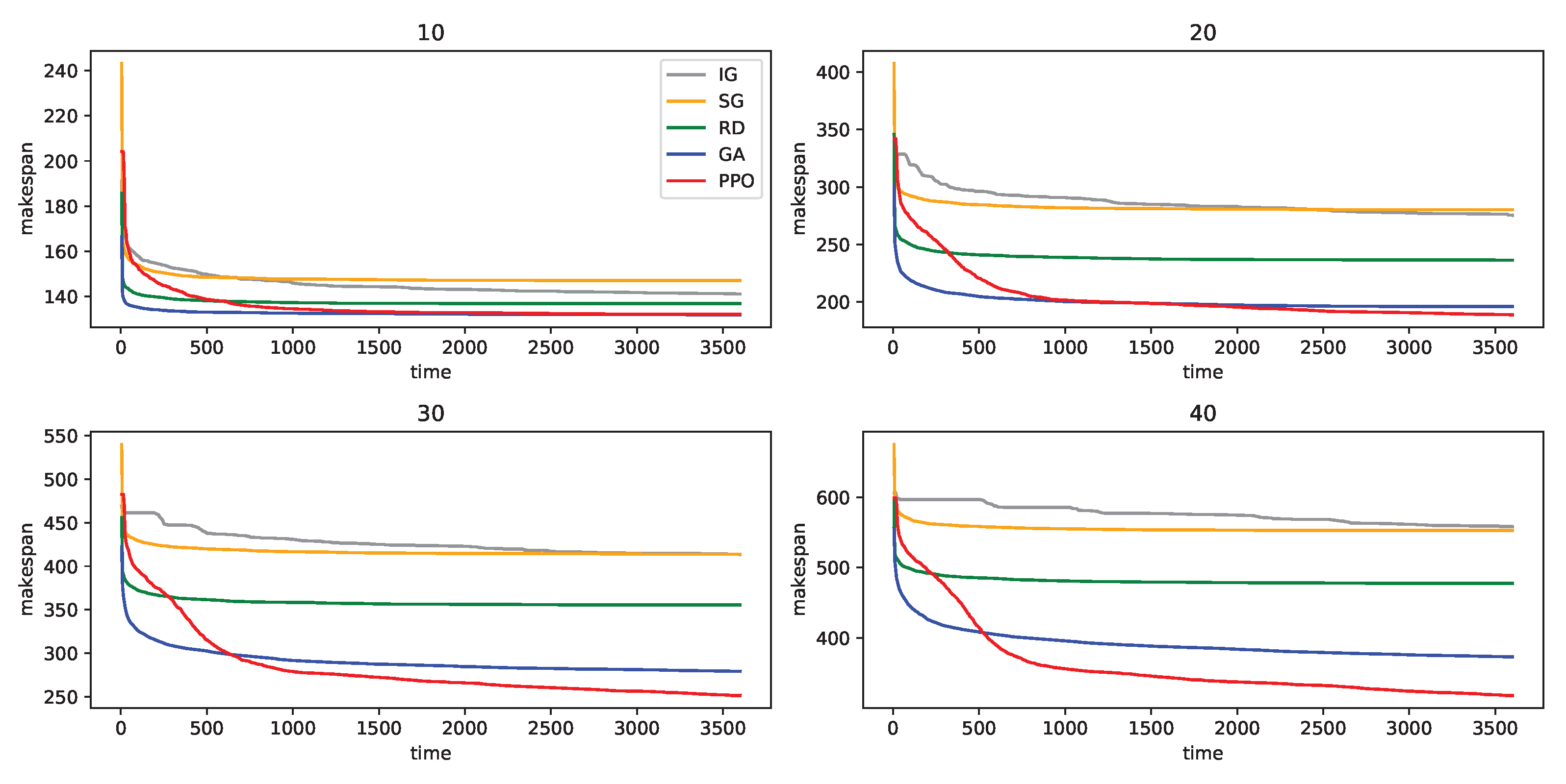
When the number of tasks is 10, the performance gap between all the algorithms is small. GA reached the minimum makespan in early step, while PPO took more than 1000 s to reach the similar performance. When the number of tasks is 20, PPO shows better performance than GA at 3600 s. However, the performance gap is not that big and we may prefer GA than PPO, if we just consider time and performance together. In the case of 30 and 40 number of tasks, PPO shows better performance at 600 s and even the performance gap between GA and PPO increases as training goes on.
Appendix A.2. Training Details
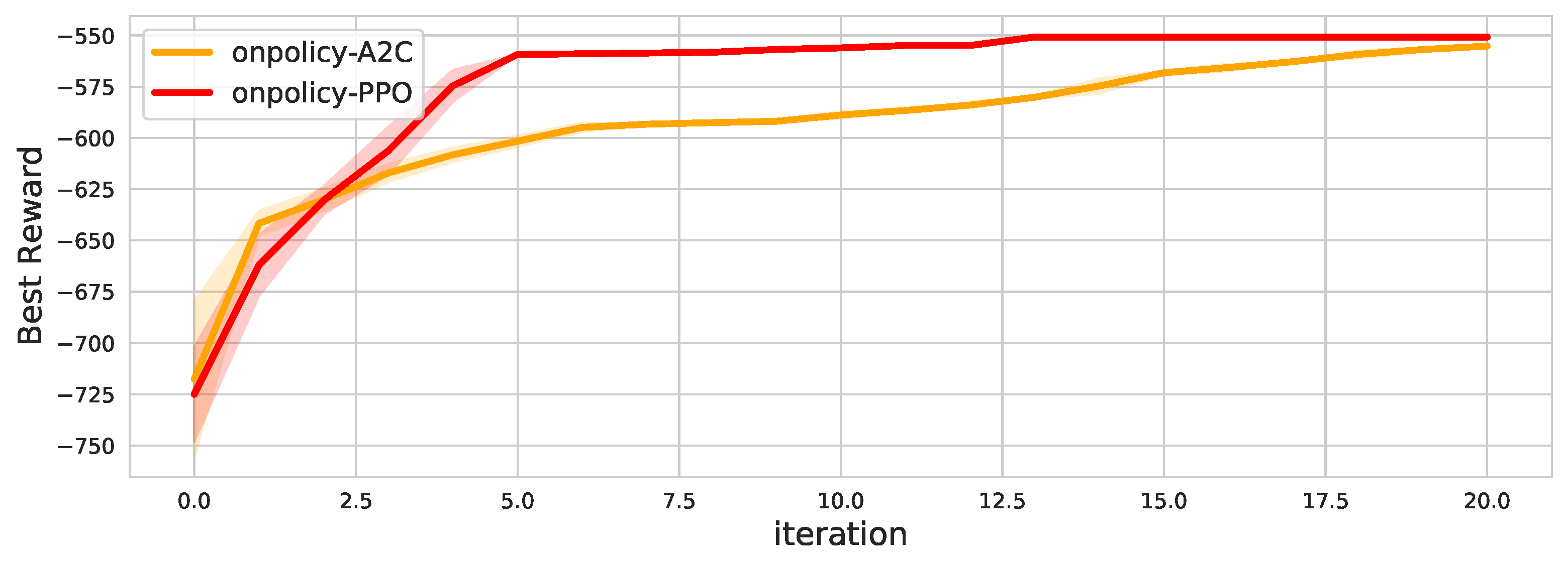
We present the hyperparameters for the model and the training in Table A1. In the case of the robot and task embedding, we used 2 linear layers for the better vector representation. Our reward scheme is only valid when an episode is finished. Therefore, we used full episode to train the model. For example, if batch size is 32 and we sampled 3 episodes with elapsed 31 time steps, then we run another episode and construct time steps larger than the batch size. We also present the effect of the model size in Figure A2. This training graph shows that there is an appropriate model size for the problem. The result suggests that there is an appropriate model size for the problem. We also tested A2C policy network as shown in the Figure A3. This result suggest that A2C on-policy method shows different learning curve.
Table A1.
Model and training hyperparameters used for experiments.
Table A1.
Model and training hyperparameters used for experiments.
| Hyperparameter | Value |
|---|---|
| Robot Embedding | 7 |
| Task Embedding | 7 |
| Robot Hidden Size 1 | 64 |
| Robot Hidden Size 2 | 128 |
| Task Hidden Size 1 | 64 |
| Task Hidden Size 2 | 128 |
| Number of Heads | 8 |
| Learning Rate | |
| Discount Rate | |
| Batch Size | 256 |
| Epsilon for PPO |

Figure A2.
Effect of the size of the hidden dimension for 20 samples in 5 robots and 50 tasks problem.
Figure A2.
Effect of the size of the hidden dimension for 20 samples in 5 robots and 50 tasks problem.
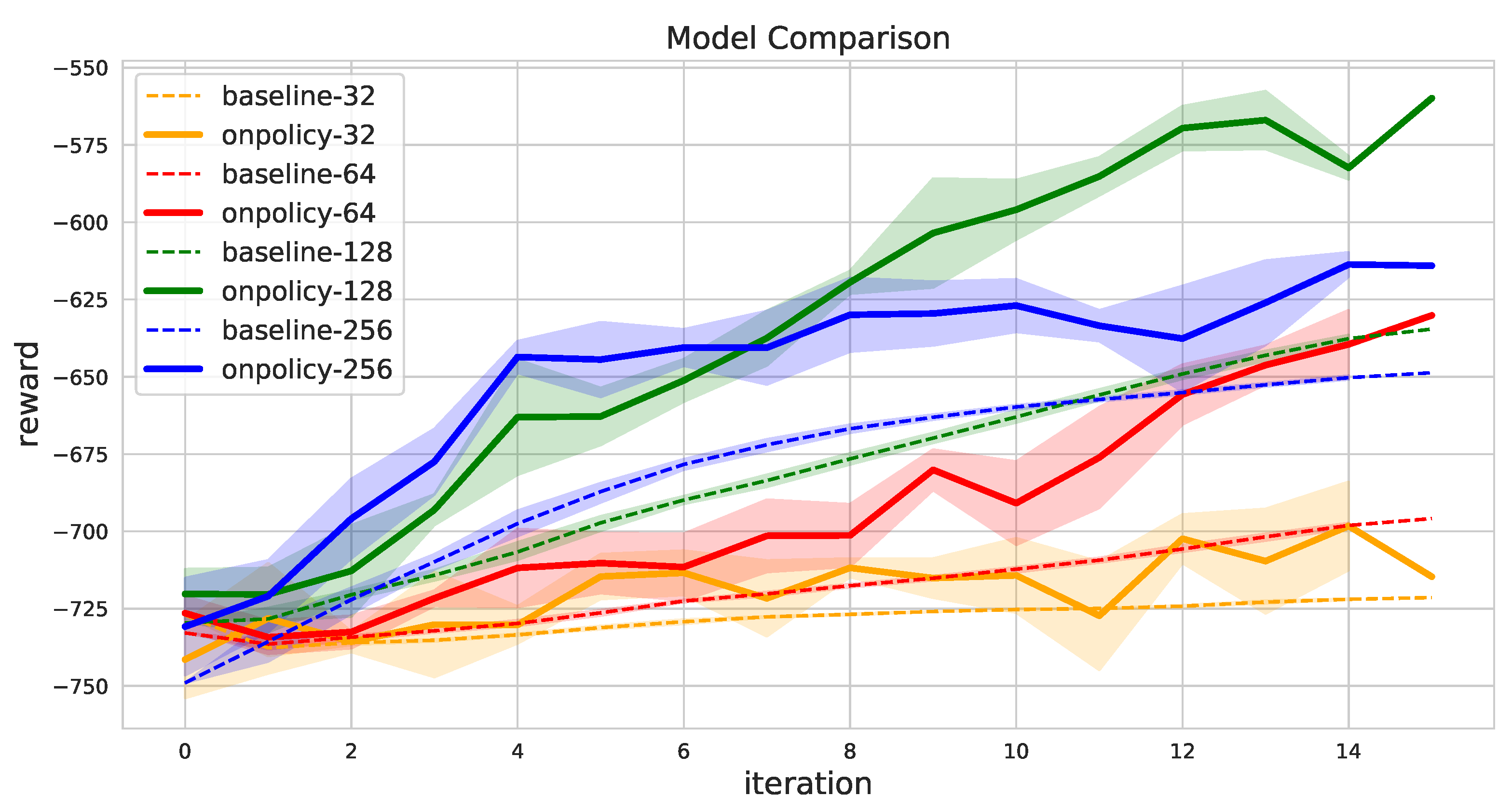
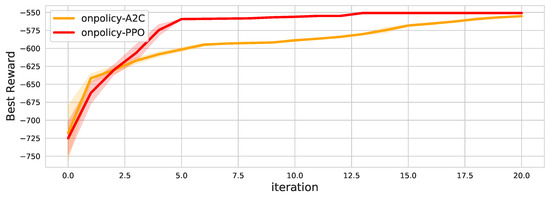
Figure A3.
Effect of policy network for 20 samples in 5 robots and 50 tasks problem.
Figure A3.
Effect of policy network for 20 samples in 5 robots and 50 tasks problem.
Appendix A.3. Comparison between Mixed Integer Programming and RL Environment
Before training in the RL environment, it is necessary to check whether the mixed integer programming formulation and the discrete-time step environment match or not. Therefore we compare the solution of branch and bound method of the mixed integer programming and meta-heuristic in the RL environment. We test on 100 random problem instances with 3 robots and 3 tasks in map size 100 and uniform workload in . There are possible permutations of allocation. Even meta-heuristic algorithms improve solutions gradually, it is not guaranteed to find the optimal solution. Hence we run enough iteration for the meta-heuristics. We set 500 iterations and 10 population-size for GA. The makespan ratios of GA and LP solution are shown in the Figure A4. As a result, the gap between the two solutions is small. The difference between LP and GA is shown in Figure A5. There are some samples whose makespan is shorter than the optimal solution. That is, the makespan of the optimal solution in MIP formulation is larger than the sub-optimal solution in MDP formulation. This mismatch is because we construct RL environment based on the MDP formulation while the optimal solution is from the MIP formulation. Specifically, the MDP formulation considers time steps as discrete values, whereas the MIP formulation has continuous values.
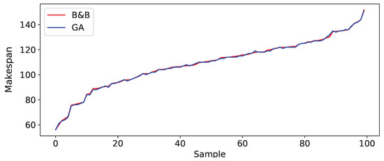
Figure A4.
The optimal makespan for 100 sample problems found by B&B in the mathematical formulation and the sub-optimal solution found by GA in the environment of 3 robots and 3 tasks. X-axis represents the index of samples sorted by the B&B makespan.
Figure A4.
The optimal makespan for 100 sample problems found by B&B in the mathematical formulation and the sub-optimal solution found by GA in the environment of 3 robots and 3 tasks. X-axis represents the index of samples sorted by the B&B makespan.
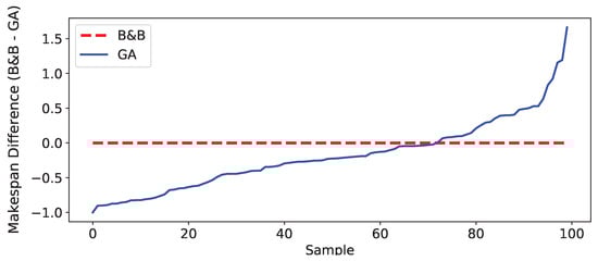
Figure A5.
The difference of makespan in Figure A4. Note that there are some samples whose performance is better than the optimal solution which represents the gap between the mixed integer programming formulation and the RL environment.
Figure A5.
The difference of makespan in Figure A4. Note that there are some samples whose performance is better than the optimal solution which represents the gap between the mixed integer programming formulation and the RL environment.
References
- Gerkey, B.P.; Matarić, M.J. A formal analysis and taxonomy of task allocation in multi-robot systems. Int. J. Robot. Res. 2004, 23, 939–954. [Google Scholar] [CrossRef] [Green Version]
- Korsah, G.A.; Stentz, A.; Dias, M.B. A comprehensive taxonomy for multi-robot task allocation. Int. J. Robot. Res. 2013, 32, 1495–1512. [Google Scholar] [CrossRef]
- Nunes, E.; Manner, M.; Mitiche, H.; Gini, M. A taxonomy for task allocation problems with temporal and ordering constraints. Robot. Auton. Syst. 2017, 90, 55–70. [Google Scholar] [CrossRef] [Green Version]
- Olson, E.; Strom, J.; Morton, R.; Richardson, A.; Ranganathan, P.; Goeddel, R.; Bulic, M.; Crossman, J.; Marinier, B. Progress toward multi-robot reconnaissance and the MAGIC 2010 competition. J. Field Robot. 2012, 29, 762–792. [Google Scholar] [CrossRef] [Green Version]
- Quann, M.; Ojeda, L.; Smith, W.; Rizzo, D.; Castanier, M.; Barton, K. An energy-efficient method for multi-robot reconnaissance in an unknown environment. In Proceedings of the 2017 American Control Conference (ACC), Seattle, WA, USA, 24–26 May 2017; pp. 2279–2284. [Google Scholar]
- Koes, M.; Nourbakhsh, I.; Sycara, K. Constraint optimization coordination architecture for search and rescue robotics. In Proceedings of the 2006 IEEE International Conference on Robotics and Automation, 2006. ICRA 2006, Orlando, FL, USA, 15–19 May 2006; pp. 3977–3982. [Google Scholar]
- Luo, C.; Espinosa, A.P.; Pranantha, D.; De Gloria, A. Multi-robot search and rescue team. In Proceedings of the 2011 IEEE International Symposium on Safety, Security, and Rescue Robotics, Kyoto, Japan, 1–5 November 2011; pp. 296–301. [Google Scholar]
- Wawerla, J.; Vaughan, R.T. A fast and frugal method for team-task allocation in a multi-robot transportation system. In Proceedings of the 2010 IEEE International Conference on Robotics and Automation, Anchorage, AK, USA, 3–7 May 2010; pp. 1432–1437. [Google Scholar]
- Eoh, G.; Jeon, J.D.; Choi, J.S.; Lee, B.H. Multi-robot cooperative formation for overweight object transportation. In Proceedings of the 2011 IEEE/SICE International Symposium on System Integration (SII), Kyoto, Japan, 20–22 December 2011; pp. 726–731. [Google Scholar]
- Nallusamy, R.; Duraiswamy, K.; Dhanalaksmi, R.; Parthiban, P. Optimization of non-linear multiple traveling salesman problem using k-means clustering, shrink wrap algorithm and meta-heuristics. Int. J. Nonlinear Sci. 2010, 9, 171–177. [Google Scholar]
- Toth, P.; Vigo, D. Vehicle Routing: Problems, Methods, and Applications; SIAM: Philadelphia, PA, USA, 2014. [Google Scholar]
- Dias, M.B.; Zlot, R.; Kalra, N.; Stentz, A. Market-based multirobot coordination: A survey and analysis. Proc. IEEE 2006, 94, 1257–1270. [Google Scholar] [CrossRef] [Green Version]
- Schneider, E.; Sklar, E.I.; Parsons, S.; Özgelen, A.T. Auction-based task allocation for multi-robot teams in dynamic environments. In Lecture Notes in Computer Science, Conference Towards Autonomous Robotic Systems; Springer: Cham, Switzerland, 2015; pp. 246–257. [Google Scholar]
- Ghassemi, P.; Chowdhury, S. Decentralized task allocation in multi-robot systems via bipartite graph matching augmented with fuzzy clustering. In Proceedings of the International Design Engineering Technical Conferences and Computers and Information in Engineering Conference, Quebec City, QC, Canada, 26–29 August 2018; American Society of Mechanical Engineers: New York, NY, USA, 2018; Volume 51753, p. V02AT03A014. [Google Scholar]
- Ghassemi, P.; DePauw, D.; Chowdhury, S. Decentralized dynamic task allocation in swarm robotic systems for disaster response. In Proceedings of the 2019 International Symposium on Multi-Robot and Multi-Agent Systems (MRS), New Brunswick, NJ, USA, 22–23 August 2019; pp. 83–85. [Google Scholar]
- Najafabadi, M.M.; Villanustre, F.; Khoshgoftaar, T.M.; Seliya, N.; Wald, R.; Muharemagic, E. Deep learning applications and challenges in big data analytics. J. Big Data 2015, 2, 1–21. [Google Scholar] [CrossRef] [Green Version]
- Banan, A.; Nasiri, A.; Taheri-Garavand, A. Deep learning-based appearance features extraction for automated carp species identification. Aquac. Eng. 2020, 89, 102053. [Google Scholar] [CrossRef]
- Fan, Y.; Xu, K.; Wu, H.; Zheng, Y.; Tao, B. Spatiotemporal modeling for nonlinear distributed thermal processes based on KL decomposition, MLP and LSTM network. IEEE Access 2020, 8, 25111–25121. [Google Scholar] [CrossRef]
- Shamshirband, S.; Rabczuk, T.; Chau, K.W. A survey of deep learning techniques: Application in wind and solar energy resources. IEEE Access 2019, 7, 164650–164666. [Google Scholar] [CrossRef]
- Afan, H.A.; Ibrahem Ahmed Osman, A.; Essam, Y.; Ahmed, A.N.; Huang, Y.F.; Kisi, O.; Sherif, M.; Sefelnasr, A.; Chau, K.W.; El-Shafie, A. Modeling the fluctuations of groundwater level by employing ensemble deep learning techniques. Eng. Appl. Comput. Fluid Mech. 2021, 15, 1420–1439. [Google Scholar] [CrossRef]
- Vinyals, O.; Fortunato, M.; Jaitly, N. Pointer Networks. Adv. Neural Inf. Processing Syst. 2015, 28, 2692–2700. [Google Scholar]
- Kool, W.; van Hoof, H.; Welling, M. Attention, Learn to Solve Routing Problems! arXiv 2019, arXiv:1803.08475. [Google Scholar]
- McClellan, M.; Cervelló-Pastor, C.; Sallent, S. Deep learning at the mobile edge: Opportunities for 5G networks. Appl. Sci. 2020, 10, 4735. [Google Scholar] [CrossRef]
- Vaswani, A.; Shazeer, N.; Parmar, N.; Uszkoreit, J.; Jones, L.; Gomez, A.N.; Kaiser, Ł.; Polosukhin, I. Attention is all you need. arXiv 2017, arXiv:1706.03762. [Google Scholar]
- Dijkstra, E.W. A note on two problems in connexion with graphs. Numer. Math. 1959, 1, 269–271. [Google Scholar] [CrossRef] [Green Version]
- McIntire, M.; Nunes, E.; Gini, M. Iterated multi-robot auctions for precedence-constrained task scheduling. In Proceedings of the 2016 International Conference on Autonomous Agents & Multiagent Systems, Singapore, 9–13 May 2016; pp. 1078–1086. [Google Scholar]
- Sutton, R.S.; Barto, A.G. Reinforcement Learning: An Introduction; MIT Press: Cambridge, MA, USA, 2018. [Google Scholar]
- Yang, S.; Xu, Z.; Wang, J. Intelligent Decision-Making of Scheduling for Dynamic Permutation Flowshop via Deep Reinforcement Learning. Sensors 2021, 21, 1019. [Google Scholar] [CrossRef]


Publisher’s Note: MDPI stays neutral with regard to jurisdictional claims in published maps and institutional affiliations. |
© 2021 by the authors. Licensee MDPI, Basel, Switzerland. This article is an open access article distributed under the terms and conditions of the Creative Commons Attribution (CC BY) license (https://creativecommons.org/licenses/by/4.0/).