1. Introduction
Present-day urbanization and traffic growth could seriously threaten human health, inducing annoyance, sleep disturbance, or even ischemic heart diseases [
1], therefore the interest on environment noise reduction is quickly growing. In this context, porous media for acoustic purposes are materials made of channels, cracks, or cavities, in which sound waves pass through the foam and lose energy due to viscous and thermal effects [
2,
3]. However, porous media are not so efficient at low frequencies as they are at high ones [
4]. Such limitation is generally bypassed through the use of multi-layer arrangements [
5]; in any case, the effects of these solutions always rely on the allowable thickness or on the total mass of the soundproofing configuration [
6,
7].
In order to overcome such a constraint, low frequency performance of acoustic packages can be significantly enhanced by resorting to the use of porous media with embedded periodic inclusions acting as local resonators [
8,
9,
10]. Such a configuration represents a meta-material and provides proper dynamic filtering effects to the material, which could be beneficial for both the system dynamics and manufacturing. First proposed by Veselago [
11] for electromagnetic waves, meta-materials have found, in recent years, a wide application in the acoustic field, since the insertion of artificial structural elements with periodic pattern allows one to control the propagation of wave phenomena [
12]. Basically, the periodic geometry induces wave interference with constructive and destructive effects [
13], which may lead to an enhancement of sound-absorbing properties with respect to traditional materials, such as porous ones [
10].
Several types of meta-materials have been proposed in the relevant literature. For example, Yang et al. [
14] introduce a decorated membrane, consisting of a pretensioned elastic membrane with rigid weights adhered on its surface; Mei et al. [
15] obtain high sound absorption through a thin decorated membrane, while Yang et al. [
16] investigate its upper bound. Moreover, Chen et al. [
17,
18] propose a complete analytical model for the absorption behavior of the membrane and confirm the energy absorption limit. Many works are inspired by Helmholtz resonators; for example, Fang et al. [
19] combine several low-wavelength Helmholtz resonators in series in order to obtain an ultrasonic resonator; Wang et al. [
20] propose an ultrathin open meta-material consisting in a large orifice in each unit cell; Kumar et al. [
21] experimentally investigate a ventilated tunable acoustic meta-material to address the challenge of acoustical performance and ventilation efficiency in conventional noise barriers; and Wei et al. and Merkel et al. [
22,
23] demonstrate that Helmholtz resonators can exhibit monopolar resonances, in contrast to single decorated membranes, in which only dipole resonances occur. However, Yang et al. [
24] show that a pair of coupled decorated membranes can provide monopolar resonances, too. The application of a shift cell technique, which is a reformulation of classical Floquet–Bloch conditions, is proposed by Magliacano et al. [
25], which then consolidate the research concerning the acoustic performances of vibroacoustic treatments based on periodic patterns by embedding inclusions into a foam layer [
26,
27,
28].
Nowadays, the use of meta-materials is suitable for different applications, such as energy, civil, and transportation (aerospace, automotive, and railway) engineering fields, where space, weight, and acoustic comfort still represent key aspects. For example, foam-based meta-materials find a wide range of applications in fuselage acoustic optimization, as reported by Magliacano et al. [
29], which propose and investigate a meta-core solution made of a foam with cylindrical inclusions. However, in the same work it can be noted how the estimation of peculiar acoustic performance indicators of meta-materials, such as the percent increase of absorption coefficient or Transmission Loss (TL) peak when passing from a homogeneous medium to a material with embedded inclusions, lacks analytical formulation, therefore pushing towards the use of numerical simulations or experimental tests, with all that derives in terms of financial expenses, computational time, experimental setup, etc. For these reasons, it is reasonable to investigate alternative techniques, such as machine learning methods, which may be able to provide automated and quick estimations of the acoustic performances of meta-material packages, which may be useful in preliminary design phases or more advanced characterization tasks. Potentially, this may lead to noticeable money and time savings.
In particular, machine learning is a subset of Artificial Intelligence (AI) in which several disciplines, such as computational statistics, pattern recognition, image processing, data mining, adaptive algorithms, etc., converge. Machine learning methods allow a computational device to perform predictions in an automatic way by learning from a set of data and exploiting the information underneath, by improving the performances on a specific task from data without being explicitly programmed. A formal and more enlightening definition is given by Mitchell [
30], which states that: “A computer program is said to learn from experience
E with respect to some class of tasks
T and performance measure
P, if its performance at tasks in
T, as measured by
P, improves with experience
E”. The fact that there is not a task-specific algorithm, confers a high versatility to the approach, which allows its application in several research fields.
Thus, it is not surprising that recently, machine learning methods have received increasing attention dedicated to the analysis of the transmission and dispersion properties of periodic acoustic meta-materials, characterized by the presence of local resonators. Bianco et al. [
31] and Michalopoulou et al. [
32] provide interesting reviews on machine learning applied to acoustics. Novel functional applications in the optimal parametric design of smart tunable mechanical filters and directional waveguides involving the use of machine learning techniques are proposed by Bacigalupo et al. [
33], as well as Gurbuz et al. [
34], who use adversarial neural networks for the design of acoustic meta-materials, while the same topic is addressed, with cloaking as ultimate goal, by Shah et al. [
35] through reinforcement learning. Both genetic algorithms and neural networks models are adopted in the literature [
36], representing an effective approach in order to design acoustic meta-materials. In particular, as an efficient machine learning method, deep learning has been widely used for data classification and regression in recent years, showing good generalization performance [
37]. Ciaburro and Iannace [
38] train artificial neural networks with sound absorption coefficient measurements. Material properties are investigated by Stender et al. [
39], which reverse-engineer sound absorbing materials in order to obtain features from the absorption coefficient.
In the present work, the effectiveness of machine learning methods as tools for performing the characterization is evaluated, in terms of TL peak frequency and percent increase (with respect to the homogeneous configuration) of meta-material acoustic packages in which the porous phase is described with two different models, namely, Delany–Bazley–Miki (DBM) and Johnson–Champoux–Allard (JCA) models. In particular, the proposed acoustic package is made of an arrangement of periodic porous unit cells with perfectly rigid inclusions.
When the DBM model is used, its simplicity allows to perform the analytical design of the meta-material assembly, which returns the unit cell dimension and the airflow resistivity on the basis of target thickness and resonance frequency; successively, the TL peak percent increase, with respect to the homogeneous configuration, is numerically estimated. Both the analytical and numerical procedures are used to generate the training set, after which the characterization of the meta-material is performed via a machine learning approach.
Successively, a similar characterization task is performed, in which the porous material is described with the JCA model, that is an acceptable trade-off between description accuracy of the material and model complexity. In more detail, in this task all the model’s parameters (namely, unit cell dimension, porosity, airflow resistivity, tortuosity, viscous characteristic length, and thermal characteristic length) are provided as input features for machine learning methods, which predicts the resonance frequency of the TL peak, first, and the percent increase of the TL peak itself, then.
The use of two models describing a meta-material has a two-fold purpose: The investigation of machine learning prediction capabilities when a “simple” (DBM) and a “complex” (JCA) model is used, and the performance changes when the number of features and training samples vary according to the model. Indeed, the results prove that more complex material models allow a finer description in machine learning terms which leads to better results.
Gaussian processes are chosen as a machine learning method for this work, mainly due to their suitability to regression problems. In the second place, but not less importantly, Gaussian processes are mathematically equivalent to many well-known models (like Bayesian linear models) and are closely related to others, such as support vector machines. Moreover, the model provided is easier to handle and interpret than other counterparts and, at the same time, the method itself is easier to apply practically (it does not require plenty of decisions like architecture, activation functions, learning rate, etc.) [
40,
41].
Therefore, the aim of this work is to investigate the applicability of more manageable, practical, and interpretable machine learning methods, such as Gaussian processes, for the characterization of foam-based meta-materials, demonstrating, at the same time, the improvement of prediction performances, even though more complex phenomenological material modeling is involved. Furthermore, the effectiveness in characterization tasks is also highlighted, which may boost up the preliminary phase of material design, characterization, and optimization, contextually reducing financial expenses and computational time related to experimental tests and numerical simulations.
This work is structured as follows. First of all, the theoretical frameworks related to the characterization of the meta-material, by means of DBM and JCA models (
Section 2.1.1 and
Section 2.1.2, respectively), and to Gaussian processes (
Section 2.2) are provided.
Section 3 is dedicated to the analysis of results, in which data pre-processing and the application of the machine learning method are accomplished differently, according to the meta-material model. In particular,
Section 3.1 illustrates the procedure that allows to analytically calculate the required values of foam airflow resistivity and unit cell dimension when the DBM model is considered. After this design part, in
Section 3.2, the properties of the studied acoustic package are introduced, along with the 3-dimensional Finite Element (FE) geometries, and a parametric test campaign is performed for several setups, and test articles described with both the foam model. Successively, in
Section 3.3, Gaussian processes are applied in order to predict the TL increases at the resonance frequencies when the meta-material is described by the DBM model; the resulting error is smaller than 5%. Then, the JCA equivalent fluid model is considered (
Section 3.4), and Gaussian processes lead to even better results when using a smaller number of training examples, with respect to the DBM case. In
Section 4, the results of this investigation are commented, and some possible future expansions of the present research are evaluated.
3. Analyses and Results
This section describes the analyses performed and the results obtained;
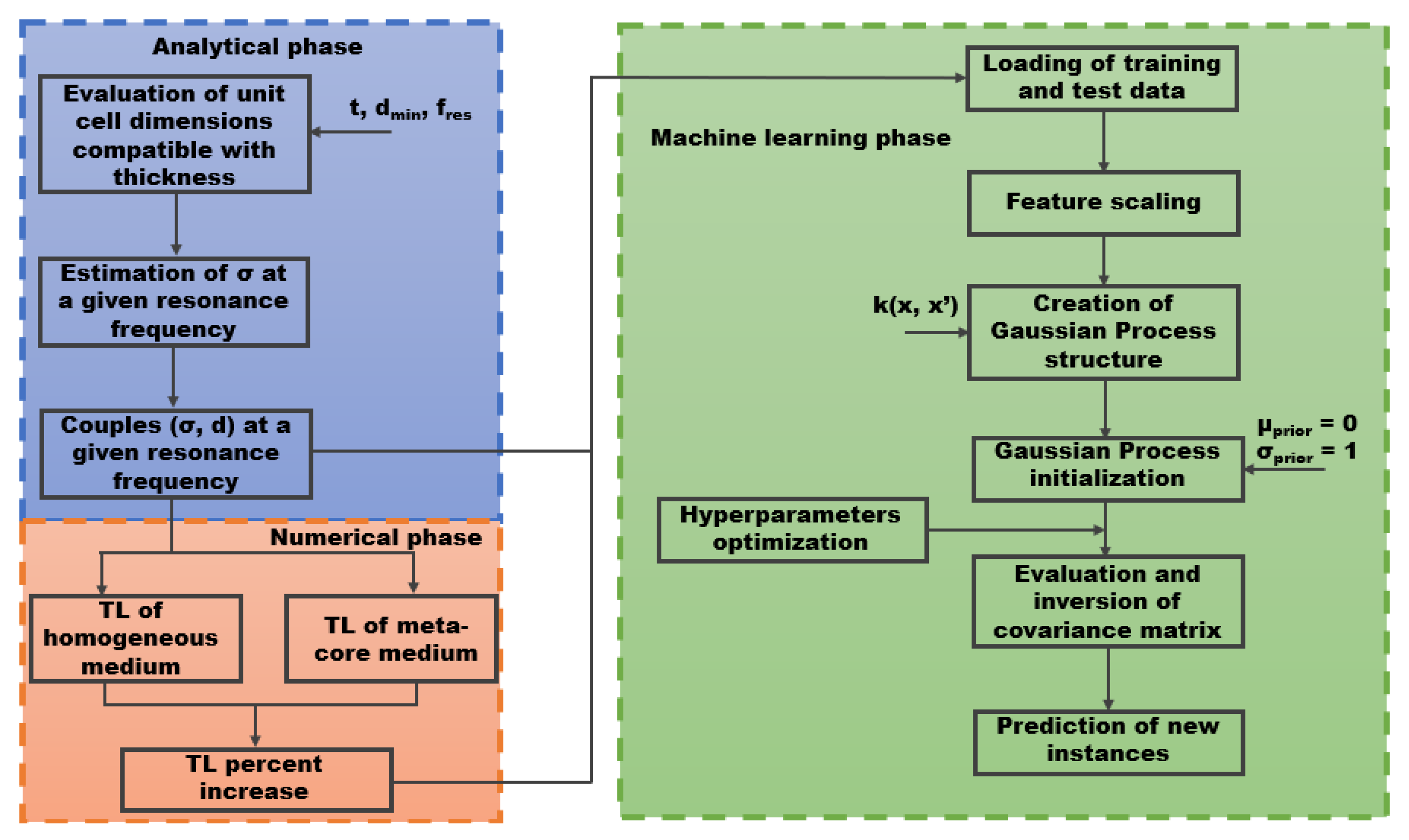
Figure 1 is a useful reference for better understanding the steps of the characterization procedure involving DBM model, explained in the following sub-sections. The other characterization task models the porous phase with the JCA model.
3.1. Analytic Part: Calculation of the Periodic Resonance Frequency
Firstly, the DBM model is used to describe the porous medium. This Section reports the analytical design procedure which, for fixed thickness and resonance frequency, returns the unit cell dimension and airflow resistivity of the model. In particular, it is illustrated how Equation (
4) is inverted in order to estimate the required foam airflow resistivity
for a desired resonance frequency. First of all, it should be pointed out that the resonance physics that is exploited herein, is linked to the well-known phenomenon that occurs when half the wavelength is equal to the periodicity dimension (namely, the unit cell dimension). So told, Equation (
4) essentially involves four quantities: The wavenumber
k, the frequency
f (and thus the angular frequency
), the speed of sound in air
(that, in this context, can be considered as a constant value), and the foam airflow resistivity
. Normally, such quantities are linked to each other such that the first one is the output, while the others are treated as inputs. In order to explicit the wavelength
, which is required for the aforementioned reason, the wavenumber
k is expressed as
; then, since in correspondence of a periodic resonance, it is verified that the dimension of periodicity,
d, is given by [
25,
26]:
in that case one may write that
. At this point, considering that the real part of a complex wavenumber is generally linked to the propagation of the wave, while the imaginary one is related to its dissipation, for the purpose of the present analysis only the real part may be taken into account. Therefore, by neglecting the imaginary part of Equation (
4) and applying the aforementioned substitutions, in correspondence of a periodic resonance one obtains:
The code used for this design phase, written in MATLAB, is based on Equation (
11) and initially asks for two geometrical constraints: The total available thickness, and the minimum unit cell dimension, which could be restrained by manufacturing aspects, and thus is limited by both lower and upper boundaries; furthermore, the prompt also requires the input of a target resonance frequency, which could fall in the whole audible range. Then, starting from the combination of the two geometrical constraints, the scripts calculates the possible numbers (and thus dimensions) of unit cells along the thickness; for each of them, the required
at the assigned resonance frequency is computed through Equation (
11). In this configuration, the script may display one or more (or even none) possible combinations of unit cell dimensions and airflow resistivity that, from a practical point of view, may lead to the choice respectively of a specific periodic pattern and foam material, with the aim of obtaining an acoustic resonance at the desired frequency.
3.2. Finite Element Part: Parametric Analysis about Airflow Resistivity and Periodicity Dimension
This Section provides the details of the FE model used to simulate the meta-material, creating both the training and test sets: The outcomes of the analytical design phase, for the DBM model, or the material parameters, for the JCA model, are provided to the FE software, which returns TLs of a homogeneous and a meta-core medium, allowing to evaluate the TL peak percent increase. These results, along with the airflow resistivity and unit cell dimension are then passed to the machine learning algorithm.
The details of the FE simulations (geometry, mesh size, number of elements, and number of nodes) used for modeling do not change whether the DBA or JCA model is used; the only difference is in the type and number of input parameters. Moreover, the foam characteristics (airflow resistivity, porosity, unit cell dimension, tortuosity, viscous, and thermal characteristic lengths), which are variable in order to generate the training and test sets, are restrained into intervals of engineering reasonability of common industrial foams. These intervals are summarized in
Table 1. The first columns reports the foam parameter, the second column lists the value intervals, and the third columns indicates the model for which they are used as input features in the machine learning phase.
The FE model is constituted by a layer of foam, with embedded periodic inclusions with the shape of cylindrical holes with perfectly rigid walls (
Figure 2); the choice of the inclusion geometry represent an example, and may eventually impact the amplitude and/or the shape of the TL resonance peak, but not its frequency (since this only depends on the foam properties and on the dimension of the periodicity). For what concerns the FE implementation, the module “Pressure Acoustics and Frequency Domain” of COMSOL MultiPhysics is used both as a modeling environment and numerical solver. For all structures presented in this work, the mesh consists of tetrahedral elements, generated through physics-controlled algorithms that are pre-implemented in the software. Nevertheless, the authors verified that the maximum element size of each HR meshed is always lower than
of the minimum wavelength
, which leads to an average number of elements through models with different sizes approximately equal to 14,250. Since the analyses are carried out considering an excitation consisting of a normal incidence plane wave acting on a layer of air (whose properties are reported in
Table 2) along the
z-axis, the only fundamental boundary condition to apply is the so-called Perfectly Matched Layer (PML) on the very bottom face of the models. Indeed, this represents an artificial absorbing layer for wave equations, commonly used to truncate computational regions in numerical methods in order to simulate problems with open boundaries; this allows the PML to strongly absorb outgoing waves from the interior of a computational region, without reflecting them back into the interior. On the contrary, boundary conditions applied on faces normal to the
x- and
y- axes are not relevant for analyses with the above-mentioned kind of excitation, since under this condition the waves do not have propagating components along those directions; thus, for the sake of computational simplicity, a Sound Hard Boundary Wall (SHBW) boundary condition is applied herein. Eventually, for different angles of excitation, proper periodic conditions should be used instead.
For a plane wave configuration at normal incidence
, and thus oriented towards the negative direction of
z-axis, the TL is computed as reported in Equation (
12):
In the context of this work, the TLs related to the homogeneous (which, obviously, has no inclusions) and the meta-core models are respectively estimated through a TMM implementation [
43] of Equations (
13) and (
14), and an FE solution of Equation (
12).
A parametric analysis is performed for all possible combinations of two chosen sets of foam airflow resistivity and unit cell dimension values. In particular, 12 airflow resistivities and 10 unit cell dimensions are selected (refer to
Table 1 for the ranges), both on a logarithmic scale, for a total of 120 different test cases; for each of them, the periodic resonance frequency (
Figure 3) is analytically calculated through the approach illustrated in
Section 3, while the TL percentage increase (
Figure 4) related the meta-core solution, compared to its homogeneous counterpart at fixed total thickness, is numerically estimated in the COMSOL environment using Equations (
12) and (
13).
For example, considering a couple of
and
d values respectively equal to 5004 kg/(sm
3) and 0.0127 m, from
Figure 3 a resonance frequency of around 13,000 Hz (the analytical value is 12,735 Hz) may be found, while from
Figure 4 an increase in the TL amplitude peak of around 150% (the FE value is 151%) may be estimated; instead, considering a couple of
and
d values respectively equal to 17,985 kg/(sm
3)] and 0.0189 m, from
Figure 3, a resonance frequency of around 8000 Hz (the analytical value is 7689 Hz) may be found, while from
Figure 4, an increase in the TL amplitude peak of around 50% (the FE value is 40%) may be estimated.
3.3. Machine Learning Part: Prediction of the Transmission Loss Increase at the Resonance Frequency (DBM Model)
The objective of this Section is to analyze the performance capabilities of Gaussian processes when predicting the TL percent increase of meta-materials (with respect to the equivalent homogeneous configuration). As already stated in
Section 2.2, the predictions on new instances are given by Equation (
7), and the estimation of the hyper-parameters is carried out with an optimization algorithm. Therefore, once the co-variance function is decided, Gaussian processes do not need any user-defined choice other than the number of training examples.
Figure 1 summarizes the several steps occurring in this phase.
Since the generation of both a numerical and/or experimental training set would be time consuming and financially expensive, there is an attempt to carry out the prediction of new instances by using the lowest number of training examples as possible; such a prediction would be considered satisfying if the percent error between the numerical and predicted peak reduction is below 5%. Moreover, in order to demonstrate the robustness of the method with the chosen number of examples, in the problem at hand, the predictions are made with three different training sets, called TS1, TS2, and TS3. To this aim, the 120 test cases numerically obtained are used as pool from which to extract training and test examples. In particular, the complete observation of each sample is made of four features: Airflow resistivity, unit cell dimension, and resonance frequency as input, while the TL peak decrease is, obviously, the output. The three sets share 20 samples, which describe the boundaries of the input space (to avoid extrapolation), to which other examples are randomly added from the aforementioned pool. The remaining elements are used for testing the generalization capabilities of the method.
Before proceeding with the learning, feature scaling is executed on all the training samples as:
where
and
are the original i-th feature and the scaled one, respectively,
is the mean value of the feature, and
is the standard deviation of the feature, both evaluated on the whole training set. This operation is almost mandatory, since the different orders of magnitude of the parameters involved may generate numerical problems during learning. Feature scaling, instead, reduces all the features to the same order of magnitude. After learning, the features are then descaled, so that the results of the predictions are made understandable to the user.
The results provided by Gaussian processes are summarized in
Figure 5. Each row displays, on the left, a 3D plot relating the three inputs (airflow resistivity, unit cell dimensions, and resonance frequency), on the cartesian axis, and the predicted peak decrease (color-coded) corresponding to each coordinate. On the right, 2D plots link the independent variables
(which provide frequency according to Equation (
4)) to the corresponding prediction error. In these figures, the black dots indicate the training examples, that must not be considered for the performance evaluation of the machine learning method.
Concerning these performances, the 2D plots show that, with a training set made of 45 samples, the prediction error remains inside the 5% boundary. The distribution of the higher errors does not follow a predictable pattern, since they not only appear in the central region of the map, but are also close to the boundaries and, sometimes, training examples. However, the same considerations hold for the lower errors.
In order to have greater insight on the performances of Gaussian processes, three test cases are considered: The analytical and numerical TL curves are provided in
Figure 6 (where the resonance frequency axis is cut at 14,000 Hz, in order to better visualize the curves and the related peaks), while
Table 3 summarizes the results in terms of reference amplitude, predicted amplitude, and prediction error for all the three training sets.
Table 3 highlights the excellent performances of Gaussian processes. More generally, TS1, TS2, and TS3 exhibit a mean percent error equal to 1.49, 1.42, and 1.66, respectively, which is much lower than the 5% boundary fixed.
3.4. Machine Learning Part: Prediction of the Resonance Frequency and Transmission Loss Increase at the Resonance Frequency (JCA Model)
The second characterization task is performed with a meta-material whose foam phase is described by the JCA model. This time, there is no analytical phase, only numerical simulations are executed in order to generate training and test sets. The input features are unit cell dimension, porosity, airflow resistivity, tortuosity, viscous characteristic length, and thermal characteristic length; the output features are TL peak frequency and percent increase.
Section 3.4 reports the results of Gaussian processes applied to meta-materials described with JCA models. In this Section, Gaussian processes are used to predict the resonance frequency and TL percent increase (at the predicted resonance frequency) of meta-materials described with the JCA model.
The JCA model allows to describe a meta-material in terms of six variables, namely: Unit cell dimension
d, porosity
, airflow resistivity
, tortuosity
, viscous characteristic length
, and thermal characteristic length
. From a machine learning point of view, such a plethora of parameters is useful fo reducing the number of training samples, thus it is expected that good predictions can be obtained with a limited number of examples for the training phase. The number of training examples is 38. Due to the high dimensionality of feature space, the description of its boundaries with samples, as performed in
Section 3.3, in order to avoid extrapolation, cannot be done since it would require the description of a six-dimensional hypervolume (and would require much more examples than those available).
The first application implies the use of a number of training examples as much as possible close to that used with the DBM model, which is 45, in order to compare the performance of the same machine learning algorithm when all other variables are retained. Thus, all the training samples are used (that is, 35), except three, used for the test phase. The input values of the test samples are reported in
Table 4, while the predictions provided by Gaussian processes, for three different training, are summarized in
Table 5 and
Table 6 for the resonance frequency and the TL peak percent increase, respectively.
The results highlight the high accuracy of the predictions the Gaussian processes are capable of providing. Comparing these outcomes with those obtained with the DBM model, since both the characterization of the Gaussian process and the number of training samples are the same (or, more precisely, the number of training samples is almost the same, being even smaller for the JCA case), it is clear that the main cause behind this improvement of performances is due to the finer characterization allowed by the JCA model, providing six input features against three in the case of the DBM model.
Hence, it is reasonable to continue the investigation in order to understand the change of the performances of the machine learning algorithm when reducing the number of training examples. Quite surprisingly, it is possible to reduce the training set to 5 samples (less samples would bring to numerical errors in the procedure) and still obtain the same quality of results, as highlighted in
Table 7 and
Table 8, reporting the predictions and errors of the same test samples.
Also in this case, the predictions accuracy is very high, exhibiting a very small percent error. Moreover, a larger picture concerning the distribution of errors (in the case of the third training) in the remaining 30 test samples is provided by the histograms in
Figure 7.
The histograms show that, in general, the errors are very low for all the other test samples. Particularly, the errors in predicting the resonance frequency are mainly concentrated in the interval 0– 4×10⁻³%, while those obtained when predicting the TL peak increase are almost totally in the interval 0–0.08%.
The last test on the performances of Gaussian processes is performed by using five training examples and removing the porosity as feature from the training set, since its values do not change significantly and, more generally, it is proven that it does not affect very much the acoustic behavior of meta-materials described with the JCA model. The predictions of the usual three test samples are listed in
Table 9 and
Table 10, and the error histograms are displayed in
Figure 8.
The results, still excellent, highlight that removing porosity does not affect significantly the performances of Gaussian processes. In particular, focusing on the histograms, the distribution of errors is mainly concentrated in the interval 0–4 × 10⁻³% for resonance frequency, and still in the interval 0–0.08% for TL percent peak increase. These outcomes demonstrate that removing a feature, which has negligible effects in the analytical model, has, actually, a corresponding outcome in the performances of machine learning algorithms. This may be used as a guideline in the choice of features for describing observations in future applications of machine learning methods.
4. Conclusions
The scope of this work is to develop and validate tools for boosting up the characterization of vibroacoustic packages based on foam cores with embedded periodic patterns through the implementation of machine learning algorithms.
First of all, the theoretical frameworks related to the characterization of the meta-material and to the chosen machine learning method are provided. Then, a procedure that allows to analytically calculate the required values of foam airflow resistivity and unit cell dimension in order to reach a desired target in terms of periodic resonance frequency is illustrated under specified constraints. Successively, the properties of the studied acoustic package are introduced, together with the 3-dimensional finite element geometries, and a parametric test campaign is performed for several setups, each with different values of foam airflow resistivity and unit cell dimension. In conclusion, a Gaussian-based machine learning algorithm is developed and applied in order to predict, with an error smaller than 5%, the Transmission Loss increases at the resonance frequencies when the DBM model is used to describe the meta-material. When the JCA model is considered, the Gaussian process can provide even better results, in predicting resonance frequencies and TL peak percent increases, with much less training examples, by increasing the number of features characterizing the observations.
Therefore, machine learning methods that are easy to handle and interpret, such as Gaussian processes, provide several advantages when meta-materials packages need characterization. In fact, the switch from DBM to JCA models demonstrates that the increase of input features leads to a noticeable reduction of the number of training examples. Hence, if one wants to generate an experimental training set, such a reduction translates into fewer samples to generate and test, and thus less money and more time savings. Moreover, important time savings are introduced in numerical simulations, since it would imply less modeling and simulations to run. All these elements help in providing automated and fast estimations of acoustic indicators, which are useful especially for investigating new configurations in preliminary design phases.
Future expansions of the present work may involve the development and implementation of more complex formulations for the description of materials, as well as advanced machine learning techniques, not only for the estimation of the acoustic performance of meta-materials, but even for their choice and optimization, according to the applications of interest. Last, but not least, it has been shown how increasing the number of features leads to an astounding level of accuracy and, at the same time, an appreciable decrease of the number of training examples. These results open the path towards the creation of an experimental training set, since the limited number of training samples would imply fewer experiments, thus time and money saving.


 ,
, 


