Analysis of Influence of Different Parameters on Numerical Simulation of NACA0012 Incompressible External Flow Field under High Reynolds Numbers

Abstract

Currently, influence analysis of simulation parameters, especially the trailing edge shape and the corresponding modeling method on the force coefficients of NACA0012 under a high Reynolds number, is relatively sparse. In this paper, two trailing edge shapes are designed by three modeling methods and combined with three far-field distances to establish eighteen two-dimensional external flow fields. The same number of structured grids are generated by a unified grid strategy and the SST k-omega and the Spalart–Allmaras models are adopted to solve the NS equations to realize the numerical simulations. Unlike under low Reynolds numbers, the analysis results show that although the accuracy difference between the sharp trailing edge and the blunt trailing edge decreases as the attack angle range increases, the former is preferred in all studied ranges. As to the corresponding modeling methods, the NACA4 and the definition formula are preferred, the choice of which depends on the studied range. In particular, a greater number of data points adopted into the definition formula is not necessarily better. Considering the error ratios comprehensively, the simulation configurations of sharp trailing edge + 20 m far-field distance + SA/SST/SST/SST/SST/SA turbulence model obtains optimal simulation effects.

1. Introduction

The accurate prediction of flight environments plays a vital role in designing and optimizing aircraft [1,2]. According to different flight velocities, the vehicle will suffer different external flow environments, including incompressible external flow fields and compressible external flow fields. The properties of a specific external flow field are different from each other, which means the corresponding parameters that need to be confirmed in the simulation prediction are also different and piecewise analysis is required. The compressible external flow field during the ascent of the vehicle is discussed in another paper by Lu and Guangming [3]; in this paper, we study the incompressible external flow field. The aircraft is immersed in the external flow field, and the fluid flowing across the airfoil surface will generate pressure in the direction perpendicular to the surface and shear force in the direction parallel to the surface. The resultant force of pressure and shear force in the flow direction is called drag, and the component perpendicular to the flow direction is called lift. The dimensionless drag coefficient ($C_d$) and lift coefficient ($C_l$) are the critical coefficients applied to characterize the drag and lift of an aircraft, research on which is of guiding significance [4]. Conventional methods can measure $C_d$ and $C_l$ through wind tunnel experiments [5], but wind tunnel experiments take a long time and are costly. With the development of computer hardware and numerical simulation technology, CFD has been adopted to solve the governing equation of fluid motion to obtain drag and lift [6,7]. This method has become the primary method to investigate the external flow field of airfoil due to its short period, high efficiency, and low cost.

The NACA airfoils developed by the National Advisory Committee for Aeronautics (NACA) are airfoil shapes for aircraft wings. NACA0012 is a typical airfoil for research on the incompressible external flow field. Ref. [8] presents CFD simulations on NACA0012, which adopts Spalart–Allmaras and SST k-omega turbulence models. The conclusion shows that the simulation data of the above turbulence models are in good agreement with published experimental data. Vassberg and Jameson [9] and Diskin, Thomas, Rumsey, and Schwoppe [10] investigate the grid strategies for the two-dimensional turbulence flow around the NACA0012 and a flat plate. Spalart–Allmaras is applied and the shape of the trailing edge is found to be a significant factor affecting the accuracy and convergence of discrete solutions. Depending on the applied modeling methods, the NACA0012 model includes the sharp trailing edge and the blunt trailing edge. In terms of the sharp trailing edge, Ref. [11] discusses the effect of the wavy surface on the aerodynamic characteristics of the NACA0012 airfoil at $R_e$ is 0.16 million, which adopts the large eddy model. Similarly, three-dimensional numerical studies on the aerodynamic characteristics with different wavy surfaces are presented in Ref. [12]. The results show that for the wavy airfoil, the $C_l$ data are reduced when the angle of attack (AOA) is less than the baseline stall angle, while when the AOA is larger than the baseline stall angle, the $C_l$ data are increased. Ref. [13] takes airfoils with a step at the upper surface and steps simultaneously at both sides of the upper and lower surfaces to investigate the effects on the aerodynamic performance. $R_e$ is 1.6 million and the turbulence model is SST k-omega. The results indicate significant changes in $C_d$ and $C_l$, and the stall angle is accrued. Devi, Paulson, Madhanraj, and Shah [14] and Li, Wang, and Zhang [15] perform similar researches by applying a square-shaped, dimpled airfoil and a Gurney flaps airfoil under $R_e$ of 2.1 million. The study shows that the NACA0012 generates a higher $C_l$ at $R_e$ of 0.283 million and 0.378 million, while this occurs at $R_e$ of 0.189 million for the flat plate.

In terms of the blunt trailing edge, Ref. [16] adopts RANS methods and the $R_e$ is 1 million. The results illustrate that the blunt trailing edge blade profile is viable for connecting structural requirements with aerodynamic performance in designing future wind turbine rotors. Ref. [17] extracts crucial quantities of the aerodynamic characteristics of a NACA0012 airfoil with the blunt trailing edge by a data-processing method, which uses the large-eddy model and an $R_e$ of 0.4 million. Through blunt trailing edge modification, the change of aerodynamic characteristics of NACA0012 is studied in Ref. [18] and the spectral analysis indicates a decrease of shedding intensity with a shorter trailing edge, with a reduction of up to 57%. In Ref. [19], the authors study the aerodynamic performance of the inflatable wing at an $R_e$ of 3 million, and the turbulence model is SST k-omega. The results show a loss of performance to a certain degree compared with the blunt trailing edge; the closer the shape, the smaller the loss of aerodynamic performance.

In summary, the researches mainly focus on the influence of geometrical changes on the force coefficients based on one trailing edge shape, and the geometrical changes include making wavy, cavity, gurney flap, cut-in sinusoidal, step, shorten, and inflatable shapes. However, the focus on the influence of the two trailing edge shapes on the simulation accuracy of force coefficients has been rarely explored, only a few papers underline the shape comparative analysis. Ref. [20] conducts a comparative study on the force coefficients under the conditions of $R_e$ of 0.189 million, 0.283 million, and 0.378 million. However, the compared objects are NACA0012 with a sharp trailing edge and a flat plate. Ref. [21] adopts the two shapes to study the influence on turbine performance under the conditions of $R_e$ of 3 million and the SST k-omega turbulence model, but the influence on the simulation accuracy of NACA0012 force coefficients is not analyzed. Ref. [22] investigates the influence of the trailing edge shape on the force coefficients applying $R_e$ from 0.05 million to 0.1 million with the SST k-omega turbulence model. The result illustrates that the chosen shape of the trailing edge depends on the values of $R_e$ and the AOA. Ref. [23] applies DNS to investigate the effect of the trailing edge shape on the characteristics of the shear layer at an $R_e$ of 0.05 million, but not on the force coefficients.

The force coefficients are affected between 3 million and 6 million [4], but the maximum $R_e$ of the above simulations is 3 million, which means that under a high $R_e$ of 6 million, the choice criteria of the trailing edge shape may be different. Unfortunately, appropriate airfoil modeling is the basis for simulation, and the above literature describes few details of the modeling methods and little attention is paid to the influence analysis of modeling methods on the simulation accuracy. Specifically, we can use Airfoil Tools, the NACA4 airfoil generator, and the definition formula to establish the NACA0012 model. For the number of the data points adopted in the definition formula, we have so far not found reliable research literature. In addition, the simulations mentioned above often adopt only one turbulence model with a fixed far-field distance, and the descriptions of the corresponding selection criteria are insufficient.

In this paper, six two-dimensional NACA0012 models, including the blunt trailing edge and the sharp trailing edge, are established based on three NACA0012 airfoil modeling methods. Then, combined with three far-field distances, eighteen external flow fields are set. The same number of structured grids are generated by a unified grid strategy and the appropriate values of mesh quality parameters are confirmed. Next, under the same boundary conditions, the corresponding CFD simulations are executed applying two turbulence models, and the numerical results of force coefficients under a high $R_e$ of 6 million are calculated. We confirm the internal relations between the above three parameters, the simulation accuracy, and the optimal simulation configurations through comparative analysis with the experimental data, which can further enrich and improve CFD research on the NACA0012 airfoil in the incompressible external flow field.

This manuscript is organized as follows. In the second section, we will briefly introduce the simulation basics of CFD. Then, in the third section, the corresponding CFD simulations are performed, applying blunt/sharp trailing edge, 12 m/16 m/20 m far-field distances, and Spalart–Allmaras/SST k-omega models. Based on the simulation results from the previous section, a detailed numerical comparison analysis is carried out in the fourth section. The last section contains conclusions.

2. Simulation Basics

2.1. NACA0012 Models

Airfoil Tools (UIUC Airfoil Coordinates Database), the NACA 4-digit airfoil generator, and the definition formula of the NACA0012 airfoil are the three standard modeling methods. Airfoil Tools provides 132 data points and the trailing edge of the designed airfoil is not closed. Therefore, it needs to be connected manually to form a blunt trailing edge. If the two points of the trailing edge are not connected manually, after being imported into modeling tools such as DesignModeler, a blunt elliptic shape will be formed at the trailing edge of the generated two-dimensional airfoil, which would fail the mesh generation. The NACA 4-digit airfoil generator supports a maximum of 200 data points and provides the close trailing edge option to design the sharp trailing edge. The definition formula of the NACA0012 is as Equation (1), where x is the X-axis location.

$$y=\pm 0.60\times [0.30\times x^{1/2}-0.13\times x-0.36\times x^2+0.30\times x^3-0.11\times x^4]$$

(1)

To compare and analyze the influence of the number of data points on the accuracy of the numerical simulation, we doubled the 132 points provided by Airfoil Tools to 264 points by adding the average value between two points. Similarly, the 200 points supplied by the NACA 4-digit airfoil generator were doubled to 400 points. Then we substituted the above four different data points into Equation (1) to establish six NACA0012 models. The chord length of the airfoil L is 1 m and the corresponding characteristic length c is 1 m as well. The six NACA0012 models are shown in Figure 1. From Figure 1b, we can see that there are apparent differences between distinct models.

Therefore, in this paper, we establish six two-dimensional NACA0012 models, including two trailing edge shapes. For the blunt trailing edge, we applied Airfoil Tools to build one NACA0012 model including 132 points. For the sharp trailing edge, five NACA0012 models were made using the following five methods: (1) NACA4-digital generator applying 200 points; (2) definition formula of NACA0012 applying 132 points provided by Airfoil Tools; (3) definition formula of NACA0012 applying 200 points provided by NACA4-digital generator; (4) definition formula of NACA0012 applying 264 points; (5) definition formula of NACA0012 applying 400 points.

2.2. Meshing

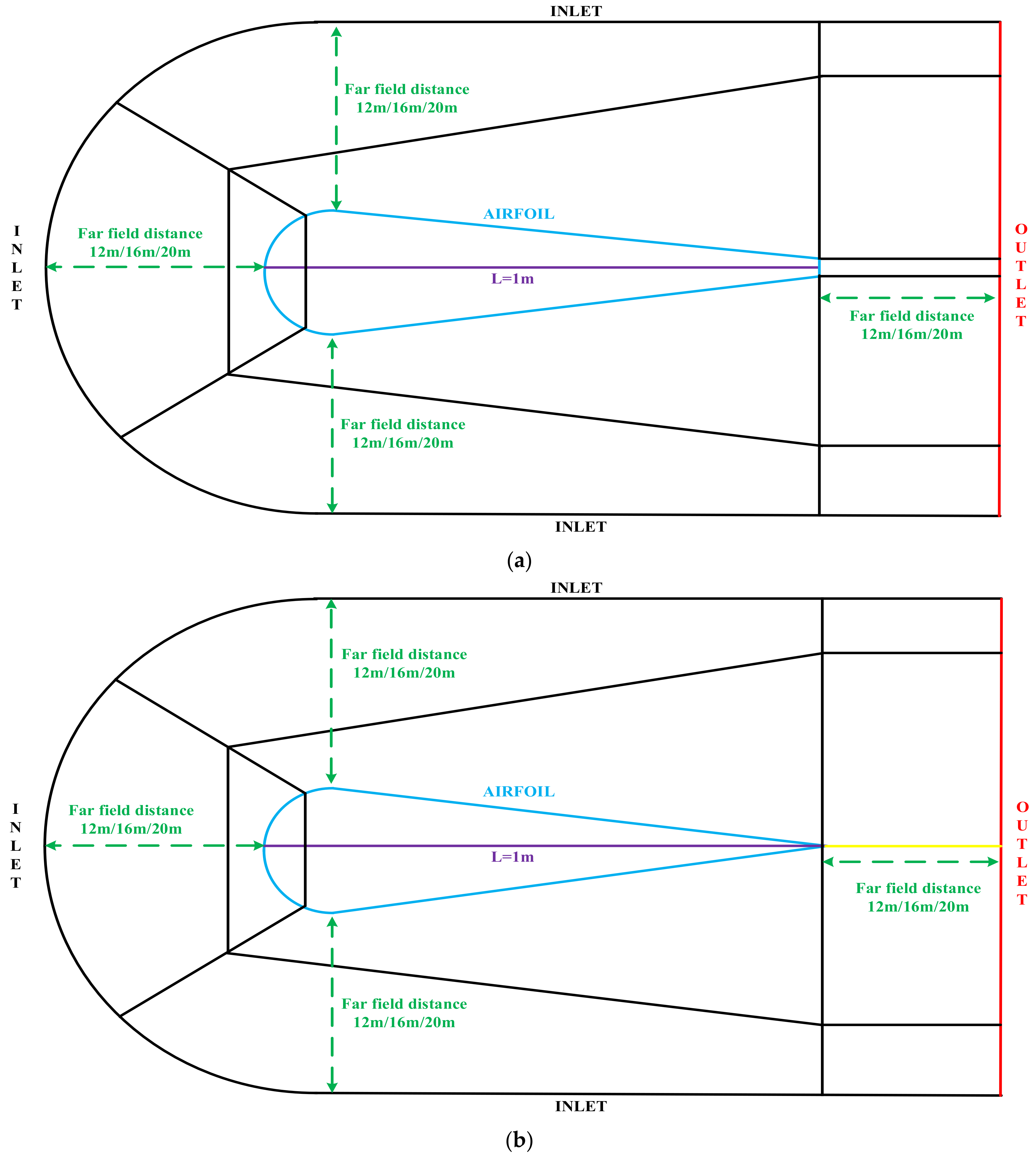
Mesh, ICEM CFD, and Pointwise are the typical meshing tools, and we apply ICEM CFD in this paper. The official recommendation is that the far-field distance for numerical simulation for the airfoil external flow field should generally be 12–20 times L [24]. In this paper, L is 1 m and 12 m/16 m/20 m were chosen to establish the C-type mesh topology in order to minimize the skewness of a near-wall mesh. As shown in Figure 2a, the mesh is similar to the “fishtail” form for the blunt trailing edge and the block at the trailing edge is retained. As shown in Figure 2b, the block is folded at the trailing edge for the sharp trailing edge. Since the height of the first layer of the boundary layer directly affects the calculation of the force coefficients, we divide the block adjacent to the airfoil wall. The input boundary of the external flow field is named INLET, the output boundary is named OUTLET, and the airfoil wall is named AIRFOIL.

2.3. Turbulence

Turbulence is a state of fluid flow in which fluid moves irregularly. The NS equations describing fluid motion is a closed system of equations and direct numerical simulation requires enormous computational resources and is challenging to apply in practice. The Reynolds average (RANS) method is widely used to average the time term of turbulence fluctuation [25]. However, at the same time, a new unknown quantity lacking the governing equation is added, which leads to the NS equations not being closed. It is necessary to select an appropriate turbulence model to close the equations describing the turbulence. The primary challenge of numerical simulation is to choose a suitable model to describe turbulence. For most numerical simulation applications, Spalart–Allmaras (SA), k-epsilon, and SST k-omega are widely accepted, along with the relatively accurate RANS turbulence models [26,27]. The Spalart–Allmaras model is explicitly designed for aeronautics and aerospace applications involving wall-bounded flows and has been shown to give good results for boundary layers subjected to adverse pressure gradients. The k-epsilon models are historically the most widely used turbulence models in industrial CFD. The draw-back of k-epsilon models is their insensitivity to adverse pressure gradients and boundary layer separation, which typically predict a delayed and reduced separation relative to observations. The k-epsilon model is therefore not widely used in external aerodynamics. The standard k-omega model in Ansys Fluent is based on a k-omega model proposed by Wilcox, the main problem of which is its strong sensitivity to freestream conditions. Therefore, the BSL k-omega model is developed to blend the robust and accurate formulation of the k-omega model in the near-wall region with the freestream independence of the k-epsilon model in the far-field. The SST k-omega model includes all the refinements of the BSL k-omega model and in addition, accounts for the transport of the turbulence shear stress in the definition of the turbulent viscosity. These features make the SST k-omega model more accurate and reliable for external flow fields of airfoils [24]. Therefore, we adopt the Spalart–Allmaras and the SST k-omega turbulence models in this paper.

Spalart–Allmaras is a one-equation RANS turbulence model, and the transport equation for the turbulent kinematic viscosity $\tilde{v}$ is

$$\frac{\partial }{\partial t}\left(\rho \tilde{v}\right)+\frac{\partial }{\partial x_i}\left(\rho \tilde{v}{u}_i\right)=\frac{1}{{\sigma }_{\tilde{v}}}\left\{\frac{\partial }{\partial x_j}\left[\left(\mu +\rho \tilde{v}\right)\frac{\partial \tilde{v}}{\partial x_j}\right]+C_{b2}\rho {\left(\frac{\partial \tilde{v}}{\partial x_j}\right)}^2\right\}+G_v-Y_v+S_{\tilde{v}}$$

(2)

Then, the turbulent viscosity ${\mu }_t$ is computed from

$${\mu }_t=\rho \tilde{v}{f}_{v1}$$

(3)

$f_{v1}$ is the viscous damping function, which is given by

$$f_{v1}=\frac{X^3}{X^3+C_{v1}^3}$$

(4)

$$X\equiv \frac{\tilde{v}}{v}$$

(5)

The model constants have default values [27].

SST k-omega is a two-equation turbulence model and the turbulent viscosity ${\mu }_t$ is computed as a function of the turbulence kinetic energy k and the specific dissipation rate $\omega$. k and $\omega$ are obtained from the following transport equations:

$$\frac{\partial }{\partial t}\left(\rho k\right)+\frac{\partial }{\partial x_i}\left(\rho k{u}_i\right)=\frac{\partial }{\partial x_j}\left({\mathsf{\Gamma }}_k\frac{\partial k}{\partial x_j}\right)+G_k-Y_k+S_k+G_b$$

(6)

$$\frac{\partial }{\partial t}\left(\rho \omega \right)+\frac{\partial }{\partial x_i}\left(\rho \omega u_i\right)=\frac{\partial }{\partial x_j}\left({\mathsf{\Gamma }}_{\omega }\frac{\partial \omega }{\partial x_j}\right)+G_{\omega }-Y_{\omega }+S_{\omega }+G_{\omega b}+D_{\omega }$$

(7)

${\mu }_t$ is given by Equation (8)

$${\mu }_t=\frac{\rho k}{\omega }\frac{1}{\max \left[\frac{1}{{\alpha }^{*}},\frac{S{F}_2}{a_1\omega }\right]}$$

(8)

where S is the strain rate magnitude and ${\alpha }^{*}$ is the turbulent viscosity damping coefficient. $F_2$ is given by

$$F_2=\tan h\left({\varphi }_2^2\right)$$

(9)

$${\varphi }_2=\max \left[2\frac{\sqrt{k}}{0.09\omega y},\frac{500\mu }{\rho y^2\omega }\right]$$

(10)

where y is the distance to the next surface. Given that the excessive generation of turbulence energy $G_k$ in the vicinity of stagnation points is a disadvantage of the SST k-omega model, the production limiters for $G_k$ are applied. The model constants have the default values [26].

$$G_k=\min \left[G_k,C_{lim}\rho \epsilon \right]$$

(11)

2.4. Numerical Procedure

For the incompressible flows, conservation equations for mass and momentum need to be solved, and we also need to solve additional transport equations for the turbulent flow. The control volume-based technique is used to discretize the above equations. Firstly, the external flow field model is divided into discrete control volumes using a computational grid. Secondly, the equations on the individual control volumes are integrated to algebraic equations for the discrete dependent variables and conserved scalars, which is accomplished using an upwind scheme. Then, the above-discretized equations are linearized, and the resultant linear equation system is solved to yield variables. The pressure-based solver is applied in this paper. More details about these equations and the finite volume method can be found in Ref. [28].

3. Numerical Simulations

At higher AOAs approaching stall, two-dimensional experimental data are difficult to achieve [4]. Considering the situation of the AOA of the aircraft during the ascending phase studied by the authors, in this paper, the minimum AOA is 0° and the maximum is 10°. There are some experimental data available. Data from Ref. [29] are not tripped; data from Ref. [30] are tripped, but are at a lower $R_e$ of 3 million. We adopt the tripped data from Ref. [31] for comparison analysis. The experimental $R_e$ is 6 million and the velocity of the freestream is about 51.3 m/s (0.15 Ma). The ambient environment is normal and Ref. [31] does not explicitly give the values of the pressure and temperature of the freestream. Referring to a NACA0012 simulation case of NASA, we assume the pressure of the freestream is 1atm and the temperature is 300 K. The computer parameters of the simulation environment are as follows: the CPU is an AMD Ryzen 7 5800X 8-core processor, the RAM is DDR4 64 G, the operating system is WIN10 64 professional version, the CFD simulation uses Ansys fluent 2020 R2, and the calculation adopts double-precision, 8-core parallel processing.

3.1. Grid Strategy

Viscosity is a measure of the internal viscosity of a fluid and all fluid flows involve some degree of viscosity effect. Viscosity causes the fluid directly in contact with the airfoil wall to be stuck to the surface without slip, called the no-slip condition. Due to the no-slip condition, within a very small normal distance adjacent to the airfoil wall, the fluid velocity will decrease from a large value to the same as the speed of the wall, resulting in a considerable gradient of the normal velocity of the wall. This area where the viscous effect causes the velocity gradient is called the boundary layer. The boundary layer is a thin viscous layer near the airfoil’s surface, containing all the viscous effects, and the flow outside the boundary layer is non-viscous. The calculation of the correlation coefficient is closely related to the viscous boundary layer. To make the numerical simulation results closer to the experimental data, the meshing of the airfoil adjacent to the wall is vitally crucial. Calculations for the height of the first layer cells of the boundary layer are begun by calculating the flow Reynolds number:

$$R_e=\frac{\rho UL}{\mu }$$

(12)

where L is the characteristic length of the airfoil, $\mu$ is the dynamic viscosity of the air, $\rho$ is the air density, and U is the freestream velocity. An empirical correlation formulation to estimate the skin friction coefficient ($C_f$) is adopted, which is for the fully developed turbulent flow over a flat plate:

$$C_f={[2{\log }_{10}(R_e)-0.65]}^{-2.3}$$

(13)

Having computed the skin friction coefficient, the wall shear stress (${\tau }_W$) is calculated:

$${\tau }_W=\frac{1}{2}\rho U^2{C}_f$$

(14)

After that, we can calculate the friction velocity ($u_{\tau }$) from the wall shear stress (${\tau }_W$):

$$u_{\tau }={(\frac{{\tau }_W}{\rho })}^{0.5}$$

(15)

The Equation for $y^{+}$ is:

$$y^{+}=\frac{\rho y_P{u}_{\tau }}{\mu }$$

(16)

Therefore, the height of the wall adjacent cell centroid from the wall ($y_P$) is:

$$y_P=\frac{y^{+}\mu }{u_{\tau }\rho }$$

(17)

Finally, the first height of the boundary layer cell ($y_H$) is double $y_P$:

$$y_H=2y_P$$

(18)

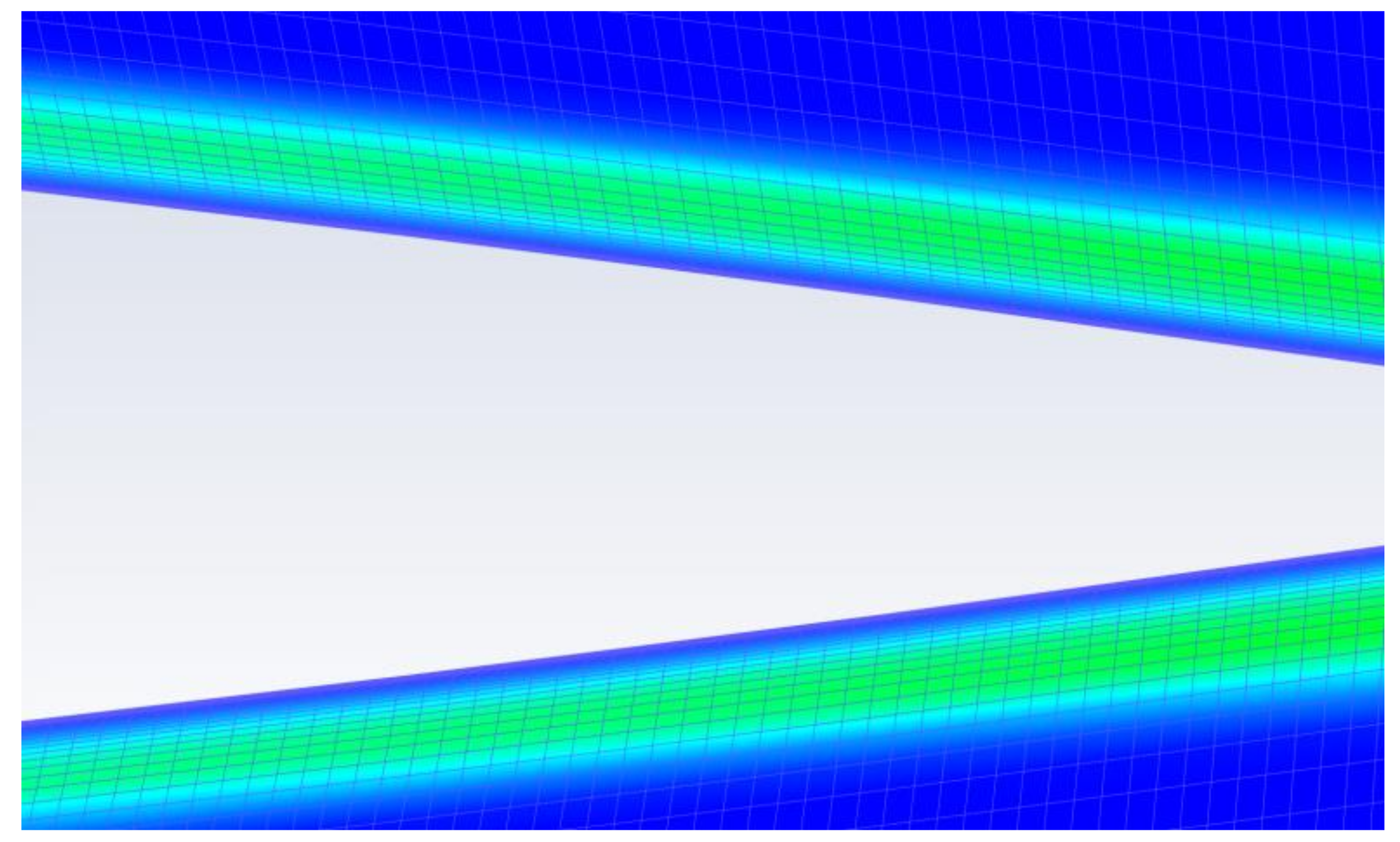
The result of the first height of the boundary layer cell is an estimate and would need to be updated using information from the CFD analysis. Ref. [24] suggests that the $y^{+}$ value should be less than 1, which could guarantee that the viscosity-affected region of the boundary layer is adequately resolved, and the first layer cells of the boundary layer should be in the sub-viscosity layer during the simulation process. The turbulent viscosity ratio (TVR) is adopted to evaluate if the boundary layer profile has been captured well. Initially, $y^{+}$ is 1 and $y_H$ is 1.53 × 10⁻⁵ m according to Equations (12)–(18), while the test results show that the maximum $y^{+}$ of airfoil surface exceeds 1 as the AOA increases during the simulation. The tests show that a $y^{+}$ value of 0.5 guarantees that the maximum $y^{+}$ of the airfoil surface stays lower than 1 during the entire simulation process, and the corresponding $y_H$ is 4.4 × 10⁻⁶ m. Figure 3 shows the corresponding plots of the TVR for the mesh with $y^{+}$ of 0.5; since the $y^{+}$ value is 0.5, there is no turbulent viscosity within the laminar sub-layer. As the mesh moves through the buffer region and into the logarithmic region, the TVR value is increased and the maximum value occurs near the middle of the boundary layer. Then, the turbulence gradually dissipates as the mesh approaches the freestream condition, which is expected. Therefore, the $y^{+}$ value is sufficient.

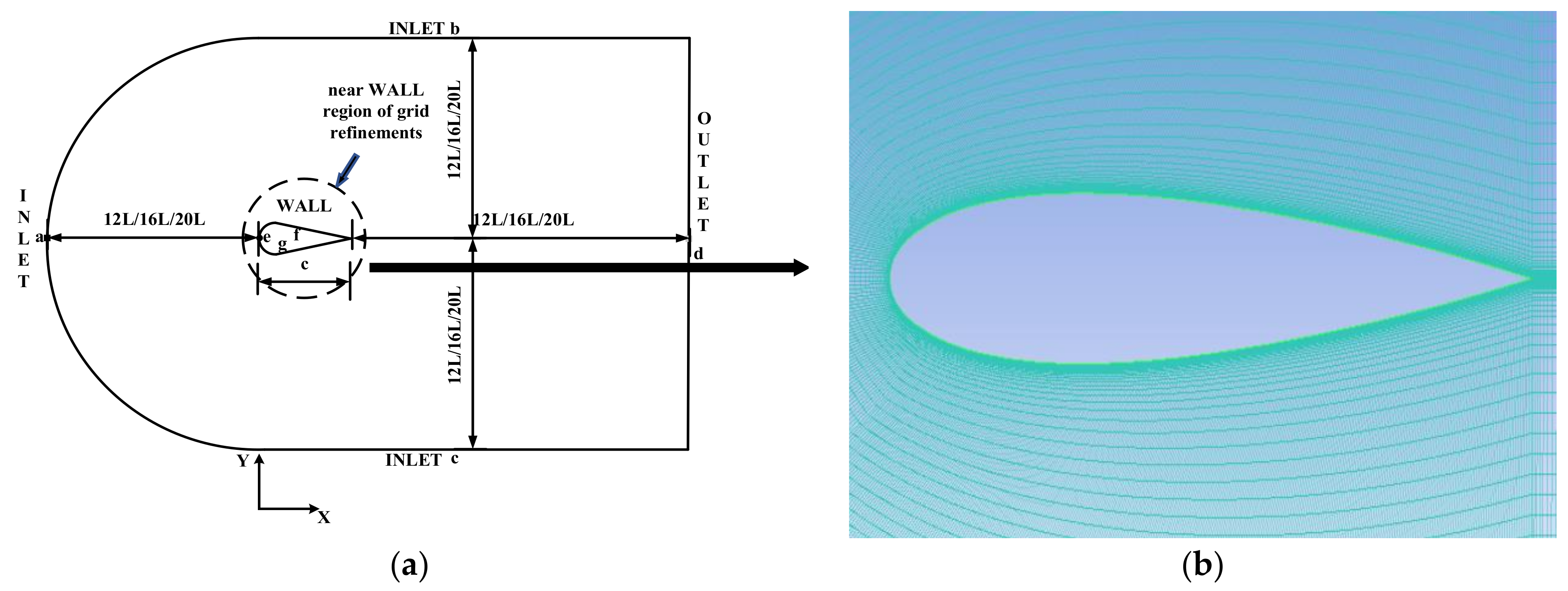
In Figure 4a, the computational domain is shown. The bold black dot is the (0,0) point of the coordinate system. The INLET boundary contains lines a, b, and c. The OUTLET boundary contains line d, and the WALL boundary has lines e, f, and g. To obtain more accurate results, more attention is needed for the grids near the WALL regions, and Figure 4b shows the close view of grids near the WALL region. Figure 5 shows the close view of grids near the blunt trailing edge and the sharp trailing edge. Three levels of grid refinement are adopted to ensure grid independency and in every refinement, the number of total grids is one times more. Taking the sharp trailing edge with the SST k-omega model as an example, the values of $C_d$, $C_l$, and error ratios are shown in

Table 1. Grid independency study of three levels of different mesh with error ratios at a far-field distance of 12 m.

Mesh (Cells)	$\mathbf{Angle} \mathbf{of} \mathbf{Attack} (°) \mathbf{and} \mathbf{Experiment} \mathbf{Data} \mathbf{of} {\mathit{C}}_{\mathit{d}}$$\mathbf{and} {\mathit{C}}_{\mathit{l}}$ $({\mathit{C}}_{\mathit{d}}$$,{\mathit{C}}_{\mathit{l}}\mathbf{and} \mathbf{Error} \mathbf{Ratios})$
	0°		2°		4°		6°		8°		10°
	0.00809	0	0.00816	0.2125	0.00823	0.4316	0.00885	0.6546	0.0105	0.8873	0.01201	1.0707
400,000	0.00791	Approx. 0	0.00836	0.21990	0.00911	0.43983	0.01044	0.64020	0.01243	0.84399	0.01529	1.03809
	2.28%	/	2.42%	3.48%	10.63%	1.91%	17.95%	2.20%	18.37%	4.88%	27.29%	3.05%
590,000	0.00799	Approx. 0	0.00823	0.21747	0.00893	0.43380	0.01013	0.64718	0.01192	0.85506	0.01437	1.05464
	1.19%	/	0.82%	2.34%	8.48%	0.51%	14.44%	1.13%	13.54%	3.63%	19.36%	1.50%
840,000	0.00801	Approx. 0	0.00831	0.21750	0.00904	0.43375	0.01034	0.64685	0.01231	0.85387	0.01515	1.04991
	0.29%	/	1.80%	2.35%	9.83%	0.50%	16.78%	1.18%	17.20%	1.50%	26.11%	1.94%

and

Table 2. Grid independency study of three levels of different mesh with error ratios at a far-field distance of 16 m.

Mesh (Cells)	$\mathbf{Angle} \mathbf{of} \mathbf{Attack} (°) \mathbf{and} \mathbf{Experiment} \mathbf{Data} \mathbf{of} {\mathit{C}}_{\mathit{d}}$$\mathbf{and} {\mathit{C}}_{\mathit{l}}$ $({\mathit{C}}_{\mathit{d}}$$,{\mathit{C}}_{\mathit{l}}\mathbf{and} \mathbf{Error} \mathbf{Ratios})$
	0°		2°		4°		6°		8°		10°
	0.00809	0	0.00816	0.2125	0.00823	0.4316	0.00885	0.6546	0.0105	0.8873	0.01201	1.0707
400,000	0.00792	Approx. 0	0.00799	0.22065	0.00895	0.43996	0.01009	0.64220	0.01191	0.84574	0.01448	1.04173
	2.16%	/	1.99%	3.83%	8.80%	1.94%	14.01%	1.89%	13.38%	4.68%	20.52%	2.71%
590,000	0.00802	Approx. 0	0.00822	0.21824	0.00886	0.43542	0.00997	0.64960	0.01165	0.85820	0.01403	1.05745
	0.91%	/	0.79%	2.70%	7.68%	0.89%	12.66%	0.76%	10.95%	3.28%	16.80%	1.24%
840,000	0.00801	Approx. 0	0.00823	0.21810	0.00887	0.43504	0.01003	0.64861	0.01180	0.85591	0.01436	1.05249
	0.96%	/	0.82%	2.64%	7.81%	0.80%	13.29%	0.91%	12.40%	3.54%	19.60%	1.70%

. As is depicted in Table 1 and Table 2, the numerical calculation results of the 590,000 and 840,000 meshes are better than those of the 400,000 meshes. In the case of the 840,000 meshes, the results are better than the 580,000 meshes only in some cases, and the range is limited. Given comprehensive consideration of computing resources and computing time, the mesh with 580,000 was applied.

The aspect ratio and the determinant are two critical indicators of the mesh evaluation parameters. In order to meet the conditions of $y^{+}$ of 0.5 and $y_H$ of 4.4 × 10⁻⁶ m, the maximum corresponding aspect ratio value would exceed 10,000 and floating-point overflow or calculation divergence may occur in the simulation process and cause the simulation to fail. In this paper, under the mesh condition with 580,000, the tests show that the maximum aspect ratio of the mesh should be within 5000, and the minimum value of the determinant should be greater than 0.8. For the blunt trailing edge, the maximum aspect ratio and the minimum value of the determinant at the far-field distance of 12 m, 16 m, and 20 m are (2200, 0.894), (2920, 0.89), and (3800, 0.863), respectively. For the sharp trailing edge, the maximum aspect ratio and the minimum value of the determinant are (1680, 0.839), (2280, 0.886), and (3640, 0.875) at the far-field distance of 12 m, 16 m, and 20 m, respectively.

3.2. Numerical Method

The Mach number M is 0.15, the static temperature of freestream T is 300 K, the dynamic viscosity $\mu$ is 1.0474 × 10⁻⁵ Pa × s, the air density is 1.225 kg/m³, and the characteristic length c is 1 m. The pressure-based solver is used with the coupled algorithm [32]. The gradients are computed according to the least-squares cell-based method. Gradients are needed not only for constructing values of a scalar at the cell faces, but also for computing secondary diffusion terms and velocity derivatives. Ansys Fluent affords cell-based and node-based schemes. The node-based scheme is known for being more accurate, particularly on skewed unstructured meshes. However, it is relatively more expensive than the cell-based scheme. Considering the limited computing resources and the applied structured meshes, the least-squares cell-based scheme is selected, which can provide comparable accuracy to that of the node-based scheme and is less expensive. The standard gradient limiter (default TVD slope limiter) [33] is adopted to prevent spurious oscillations, which uses the Minmod function (minimum modulus) to limit and clip the reconstructed solution overshoots and undershoots on the cell faces. The second-order scheme is used for interpolating the pressure values at the faces, which reconstructs the face pressure using a central differencing scheme. It should be pointed out that for the Spalart–Allmaras turbulence model, the simulation results of modified turbulent viscosity applying first-order upwind seem little better than those applying second-order upwind. Taking the sharp trailing edge and adopting Spalart–Allmaras at far-field distances of 12 m and 16 m as examples, we chose three AOAs (0°, 2°, 4°); the comparative data are shown in

Table 3. Comparative data of the modified turbulent viscosity of Spalart–Allmaras applying first-order upwind and second-order upwind.

Far-Field Distance	Type of Upwind Order	$\mathbf{Angle} \mathbf{of} \mathbf{Attack} (°) \mathbf{and} \mathbf{Experiment} \mathbf{Data} \mathbf{of} {\mathit{C}}_{\mathit{d}}$ $\mathbf{and} {\mathit{C}}_{\mathit{l}}$$({\mathit{C}}_{\mathit{d}}$$, {\mathit{C}}_{\mathit{l}}\mathbf{and} \mathbf{Error} \mathbf{Ratios})$
		0°		2°		4°
		0.00809	0	0.00816	0.2125	0.00823	0.4316
12 m	First-order	0.00809427	Approx. 0	0.00832899	0.21984088	0.00900243	0.43858932
		0.05%	/	2.07%	3.45%	9.39%	1.62%
	Second-order	0.00810023	Approx. 0	0.00833216	0.21977944	0.00900414	0.43871334
		0.13%	/	2.11%	3.43%	9.41%	1.65%
16 m	First-order	0.00811742	Approx. 0	0.00832344	0.22078817	0.00893481	0.44042730
		0.34%	/	2.00%	3.90%	8.56%	2.05%
	Second-order	0.0081189	Approx. 0	0.008322422	0.22087445	0.00892964	0.44054850
		0.36%	/	2.01%	3.94%	8.50%	2.07%

. At an AOA of 2°, although the $C_l$ error ratio of the second-order at a far-field distance of 12 m is lower than that of the first-order, the total error ratios of the first-order are preferred. Therefore, we choose the modified turbulent viscosity of Spalart–Allmaras as the first-order upwind.

The simulation parameters of convergence numerical results are as shown in

Table 4. Simulation parameters of convergence numerical results.

Validation Parameters
Solver	Pressure-based with coupled algorithm	Pressure-based with coupled algorithm
Turbulence Models	SST k-omega	Spalart–Allmaras
Materials	Density (kg/m3): 1.225 Viscosity (Pa × s): 1.0474 × 10−5	Density (kg/m3): 1.225 Viscosity (Pa × s): 1.0474 × 10−5
Initial conditions	Mach number: 0.15	Mach number: 0.15
	Static temperature: 300 K	Static temperature: 300 K
Boundary conditions	INLET: velocity-inlet	INLET: velocity-inlet
	OUTLET: pressure outlet	OUTLET: pressure outlet
	AIRFOIL: no-slip, adiabatic	AIRFOIL: no-slip, adiabatic
Spatial discretization	Gradient: least-squares cell-based	Gradient: least-squares cell-based
	Pressure: second-order	Pressure: second-order
	Momentum: second-order upwind	Momentum: second-order upwind
	Turbulent kinetic energy: second-order upwind	Modified turbulent viscosity: first-order upwind
	Specific dissipation rate: second-order upwind

. The turbulence model adopts SST k-omega and the turbulence specification method of the INLET boundary selects the intensity and viscosity ratios; the related values are 0.052% and 0.009. The turbulence model applies Spalart–Allmaras, the turbulence specification method of the INLET boundary selects the turbulent viscosity ratio, and the value is 3.

3.3. Numerical Results

Taking three AOAs (0°, 2°, 4°) as examples, the experimental data and the numerical simulation data of $C_d$ and $C_l$, with error ratios between them, under the conditions of six NACA0012 models, three far-field distances, and two turbulence models, are shown in

Table 5. Simulation results of $C_d$ and $C_l$ with error ratios adopting SST k-omega and far-field distances of 12 m and 16 m.

Type of NACA0012 Model		Angle of Attack (°) and Experiment data of ${\mathit{C}}_{\mathit{d}}$ and ${\mathit{C}}_{\mathit{l}}$ (Numerical Data of ${\mathit{C}}_{\mathit{d}}$ and ${\mathit{C}}_{\mathit{l}}$ with Error Ratios)
		12 m (SST k-omega)						16 m (SST k-omega)
		0°	0.00809	2°	0.00816	4°	0.00823	0°	0.00809	2°	0.00816	4°	0.00823
			0		0.2125		0.4316		0		0.2125		0.4316
Blunt trailing edge (Airfoil Tools 132 points)	$C_d$	0.00806	0.37%	0.00830	1.67%	0.00901	9.50%	0.00807	0.21%	0.00829	1.62%	0.00894	8.66%
	$C_l$	Approx. 0	0.00%	0.2204	3.71%	0.4391	1.73%	Approx. 0	0.00%	0.2215	4.21%	0.4415	2.29%
Sharp trailing edge (NACA4 200 points)	$C_d$	0.00799	1.19%	0.00823	0.82%	0.00893	8.48%	0.00802	0.91%	0.00822	0.79%	0.01437	19.63%
	$C_l$	Approx. 0	0.00%	0.2175	2.34%	0.4338	0.51%	Approx. 0	0.00%	0.2182	2.70%	1.0546	1.50%
Sharp trailing edge (Formula adopts 132 points)	$C_d$	0.00799	1.26%	0.00822	0.79%	0.00893	8.48%	0.00800	1.11%	0.00821	0.57%	0.01450	20.71%
	$C_l$	Approx. 0	0.00%	0.2178	2.50%	0.4348	0.74%	Approx. 0	0.00%	0.2187	2.90%	1.0564	1.33%
Sharp trailing edge (Formula adopts 200 points)	$C_d$	0.00799	1.30%	0.00822	0.69%	0.00892	8.38%	0.00800	1.12%	0.00821	0.61%	0.01451	20.78%
	$C_l$	Approx. 0	0.00%	0.2178	2.50%	0.4347	0.73%	Approx. 0	0.00%	0.2186	2.86%	1.0556	1.41%
Sharp trailing edge (Formula adopts 264 points)	$C_d$	0.00799	1.21%	0.00823	0.84%	0.00894	8.66%	0.00800	1.06%	0.00822	0.70%	0.01477	22.96%
	$C_l$	Approx. 0	0.00%	0.2178	2.50%	0.4346	0.69%	Approx. 0	0.00%	0.2185	2.83%	1.0532	1.64%
Sharp trailing edge (Formula adopts 400 points)	$C_d$	0.00799	1.21%	0.00823	0.85%	0.00894	8.57%	0.00801	1.04%	0.00821	0.64%	0.01454	21.04%
	$C_l$	Approx. 0	0.00%	0.2178	2.50%	0.4347	0.72%	Approx. 0	0.00%	0.2186	2.86%	1.0558	1.40%

,

Table 6. Simulation results of ${\mathit{C}}_{\mathit{d}}$ and ${\mathit{C}}_{\mathit{l}}$ with error ratios adopting SST k-omega and a far-field distance of 20 m, adopting Spalart–Allmaras and a far-field distance of 12 m.

Type of NACA0012 Model		Angle of Attack (°) and Experiment Data of ${\mathit{C}}_{\mathit{d}}$ and ${\mathit{C}}_{\mathit{l}}$ (Numerical Data of ${\mathit{C}}_{\mathit{d}}$ and ${\mathit{C}}_{\mathit{l}}$ with Error Ratios)
		20 m (SST k-omega)						12 m (Spalart–Allmaras)
		0°	0.00809	2°	0.00816	4°	0.00823	0°	0.00809	2°	0.00816	4°	0.00823
			0		0.2125		0.4316		0		0.2125		0.4316
Blunt trailing edge (Airfoil Tools 132 points)	$C_d$	0.00820	1.30%	0.00826	1.26%	0.00887	7.73%	0.00816	0.80%	0.00839	2.79%	0.00907	10.24%
	$C_l$	Approx. 0	0.00%	0.2201	3.57%	0.4389	1.68%	Approx. 0	0.00%	0.2214	4.18%	0.4412	2.22%
Sharp trailing edge (NACA4 200 points)	$C_d$	0.00799	1.19%	0.00819	0.36%	0.00879	6.84%	0.00809	0.05%	0.00833	2.07%	0.01388	15.56%
	$C_l$	Approx. 0	0.00%	0.2184	2.76%	0.4355	0.91%	Approx. 0	0.00%	0.2198	3.45%	1.0560	1.37%
Sharp trailing edge (Formula adopts 132 points)	$C_d$	0.00800	1.05%	0.00820	0.50%	0.00880	6.88%	0.00808	0.18%	0.00830	1.73%	0.01375	14.47%
	$C_l$	Approx. 0	0.00%	0.2190	3.07%	0.4370	1.25%	Approx. 0	0.00%	0.2201	3.55%	1.0606	0.94%
Sharp trailing edge (Formula adopts 200 points)	$C_d$	0.00800	1.08%	0.00820	0.53%	0.00881	7.02%	0.00809	0.04%	0.00832	1.91%	0.01394	16.11%
	$C_l$	Approx. 0	0.00%	0.2191	3.09%	0.4368	1.21%	Approx. 0	0.00%	0.2198	3.45%	1.0583	1.16%
Sharp trailing edge (Formula adopts 264 points)	$C_d$	0.00800	1.07%	0.00820	0.50%	0.00880	6.89%	0.00808	0.13%	0.00831	1.79%	0.01374	14.39%
	$C_l$	Approx. 0	0.00%	0.2190	3.05%	0.4369	1.23%	Approx. 0	0.00%	0.2201	3.56%	1.0606	0.95%
Sharp trailing edge (Formula adopts 400 points)	$C_d$	0.00800	1.06%	0.00820	0.51%	0.00880	6.91%	0.00808	0.15%	0.00830	1.77%	0.01373	14.32%
	$C_l$	Approx. 0	0.00%	0.2190	3.04%	0.4369	1.22%	Approx. 0	0.00%	0.2200	3.54%	1.0608	0.92%

and

Table 7. Simulation results of $C_d$ and $C_l$ with error ratios adopting Spalart–Allmaras and far-field distances of 16 m and 20 m.

Type of NACA0012 Model		Angle of Attack (°) and Experiment Data of ${\mathit{C}}_{\mathit{d}}$ and ${\mathit{C}}_{\mathit{l}}$ (Numerical Data of ${\mathit{C}}_{\mathit{d}}$ and ${\mathit{C}}_{\mathit{l}}$ with Error Ratios)
		16 m (Spalart–Allmaras)						20 m (Spalart–Allmaras)
		0°	0.00809	2°	0.00816	4°	0.00823	0°	0.00809	2°	0.00816	4°	0.00823
			0		0.2125		0.4316		0		0.2125		0.4316
Blunt trailing edge (Airfoil Tools 132 points)	$C_d$	0.00820	1.31%	0.00841	3.04%	0.00903	9.71%	0.00816	0.84%	0.00835	2.34%	0.00893	8.46%
	$C_l$	Approx. 0	0.00%	0.2222	4.57%	0.4432	2.68%	Approx. 0	0.00%	0.2215	4.23%	0.4422	2.46%
Sharp trailing edge (NACA4 200 points)	$C_d$	0.00812	0.34%	0.00832	2.00%	0.00893	8.56%	0.00809	0.06%	0.00829	1.60%	0.01380	14.90%
	$C_l$	Approx. 0	0.00%	0.2208	3.90%	0.4404	2.05%	Approx. 0	0.00%	0.2213	4.15%	1.0731	0.23%
Sharp trailing edge (Formula adopts 132 points)	$C_d$	0.00808	0.11%	0.00828	1.45%	0.00889	7.98%	0.00809	0.02%	0.00828	1.43%	0.01378	14.71%
	$C_l$	Approx. 0	0.00%	0.2209	3.93%	0.4406	2.08%	Approx. 0	0.00%	0.2213	4.14%	1.0735	0.27%
Sharp trailing edge (Formula adopts 200 points)	$C_d$	0.00808	0.08%	0.00828	1.52%	0.00890	8.10%	0.00809	0.00%	0.00828	1.45%	0.01379	14.79%
	$C_l$	Approx. 0	0.00%	0.2208	3.90%	0.4404	2.05%	Approx. 0	0.00%	0.2213	4.15%	1.0731	0.23%
Sharp trailing edge (Formula adopts 264 points)	$C_d$	0.00808	0.09%	0.00829	1.57%	0.00891	8.24%	0.00809	0.01%	0.00828	1.43%	0.01397	16.34%
	$C_l$	Approx. 0	0.00%	0.2207	3.87%	0.4404	2.03%	Approx. 0	0.00%	0.2213	4.13%	1.0713	0.06%
Sharp trailing edge (Formula adopts 400 points)	$C_d$	0.00809	0.05%	0.00831	1.79%	0.00892	8.41%	0.00809	0.05%	0.00828	1.46%	0.01386	15.38%
	$C_l$	Approx. 0	0.00%	0.2206	3.82%	0.4401	1.96%	Approx. 0	0.00%	0.2213	4.12%	1.0726	0.18%

.

4. Results and Discussion

According to the CFD simulation results obtained in Section 3, we can discuss the influence of different parameters on the numerical simulation in three aspects: the NACA0012 models, the far-field distances, and the turbulence models. NACA0012 is a symmetrical airfoil; the $C_l$ is 0 when the AOA is 0° and the magnitude of the simulation result of $C_l$ is 10⁻⁶, which approximately approaches 0. Therefore, the error ratio of $C_l$ is about 0.00% when the AOA is 0°.

4.1. Results of NACA0012 Models

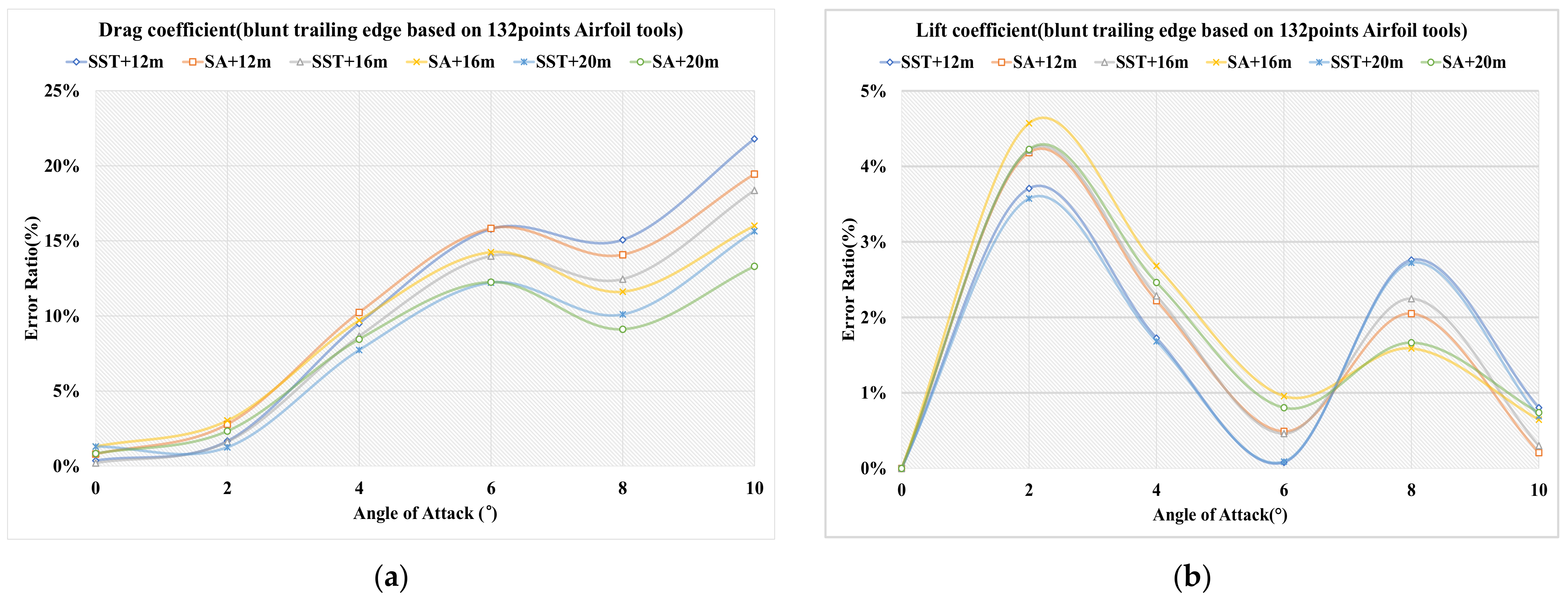
Based on the SST k-omega and Spalart–Allmaras turbulence models and 12 m/16 m/20 m far-field distances, we made six simulation configurations: SST+12 m, SST+16 m, SST+20 m, SA+12 m, SA+16 m, and SA+20 m. Then, applying the simulation parameters described in Table 4, for each NACA0012 model, six groups of simulations were performed and the results of the error ratios compared with the experimental data are illustrated in Figure 6, Figure 7, Figure 8, Figure 9, Figure 10 and Figure 11. The figures show that the error ratios under different configurations change with the AOA changes. Therefore, at the AOA ranges (0°, 0°), (0°, 2°), (0°, 4°), (0°, 6°), (0°, 8°), and (0°, 10°), we can calculate the mean error ratios; the results are provided in

Table 8. The mean error ratios of $C_d$ and $C_l$ of the blunt trailing edge.

Simulation Configurations	Range of AOA(°)
	$\mathbf{Mean} \mathbf{Error} \mathbf{Ratios} \mathbf{of} ({\mathit{C}}_{\mathit{d}}$$,{\mathit{C}}_{\mathit{l}})$
	(0°, 0°)	(0°, 2°)	(0°, 4°)	(0°, 6°)	(0°, 8°)	(0°, 10°)
SST+12 m	(0.37%, 0.00%)	(1.02%, 1.85%)	(3.85%, 1.81%)	(6.83%, 1.38%)	(8.48%, 1.66%)	(10.70%, 1.51%)
SST+16 m	(0.21%, 0.00%)	(0.92%, 2.11%)	(3.50%, 2.17%)	(6.12%, 1.74%)	(7.39%, 1.84%)	(9.22%, 1.59%)
SST+20 m	(1.30%, 0.00%)	(1.28%, 1.79%)	(3.43%, 1.75%)	(5.63%, 1.34%)	(6.52%, 1.61%)	(8.04%, 1.46%)
SA+12 m	(0.80%, 0.00%)	(1.80%, 2.09%)	(4.61%, 2.14%)	(7.42%, 1.72%)	(8.75%, 1.79%)	(10.54%, 1.53%)
SA+16 m	(1.31%, 0.00%)	(2.17%, 2.29%)	(4.69%, 2.42%)	(7.08%, 2.05%)	(7.98%, 1.96%)	(9.32%, 1.74%)
SA+20 m	(0.84%, 0.00%)	(1.59%, 2.11%)	(3.88%, 2.23%)	(5.97%, 1.87%)	(6.60%, 1.83%)	(7.72%, 1.65%)

,

Table 9. The mean error ratios of $C_d$ and $C_l$ of the sharp trailing edge based on NACA4-digital generator.

Simulation Configurations	Range of AOA (°)
	$\mathbf{Mean} \mathbf{Error} \mathbf{Ratios} \mathbf{of} ({\mathit{C}}_{\mathit{d}}$$,{\mathit{C}}_{\mathit{l}})$
	(0°, 0°)	(0°, 2°)	(0°, 4°)	(0°, 6°)	(0°, 8°)	(0°, 10°)
SST+12 m	(1.19%, 0.00%)	(1.01%, 1.17%)	(3.50%, 0.95%)	(6.23%, 1.00%)	(7.69%, 1.52%)	(9.68%, 1.52%)
SST+16 m	(0.91%, 0.00%)	(0.85%, 1.35%)	(3.13%, 1.20%)	(5.51%, 1.09%)	(6.60%, 1.53%)	(8.30%, 1.48%)
SST+20 m	(1.19%, 0.00%)	(0.78%, 1.38%)	(2.80%, 1.22%)	(4.98%, 1.11%)	(5.89%, 1.55%)	(7.50%, 1.52%)
SA+12 m	(0.05%, 0.00%)	(1.06%, 1.73%)	(3.84%, 1.69%)	(6.56%, 1.27%)	(7.84%, 1.50%)	(9.48%, 1.26%)
SA+16 m	(0.34%, 0.00%)	(1.17%, 1.95%)	(3.64%, 1.98%)	(5.97%, 1.59%)	(6.84%, 1.68%)	(8.18%, 1.44%)
SA+20 m	(0.06%, 0.00%)	(0.83%, 2.08%)	(3.13%, 2.14%)	(5.28%, 1.75%)	(5.98%, 1.78%)	(7.50%, 1.53%)

,

Table 10. The mean error ratios of $C_d$ and $C_l$ of the sharp trailing edge based on definition formula applying 132 points.

Simulation Configurations	Range of AOA (°)
	$\mathbf{Mean} \mathbf{Error} \mathbf{Ratios} \mathbf{of} ({\mathit{C}}_{\mathit{d}}$$,{\mathit{C}}_{\mathit{l}})$
	(0°, 0°)	(0°, 2°)	(0°, 4°)	(0°, 6°)	(0°, 8°)	(0°, 10°)
SST+12 m	(1.26%, 0.00%)	(1.03%, 1.25%)	(3.51%, 1.08%)	(6.31%, 1.04%)	(7.85%, 1.51%)	(9.99%, 1.48%)
SST+16 m	(1.11%, 0.00%)	(0.84%, 1.45%)	(3.06%, 1.32%)	(5.43%, 1.14%)	(6.56%, 1.55%)	(8.32%, 1.48%)
SST+20 m	(1.05%, 0.00%)	(0.78%, 1.54%)	(2.81%, 1.44%)	(4.93%, 1.19%)	(5.75%, 1.55%)	(7.20%, 1.45%)
SA+12 m	(0.18%, 0.00%)	(0.95%, 1.78%)	(3.67%, 1.76%)	(6.43%, 1.35%)	(7.75%, 1.54%)	(9.55%, 1.28%)
SA+16 m	(0.11%, 0.00%)	(0.78%, 1.97%)	(3.18%, 2.01%)	(5.49%, 1.62%)	(6.37%, 1.70%)	(7.76%, 1.46%)
SA+20 m	(0.02%, 0.00%)	(0.73%, 2.07%)	(2.98%, 2.14%)	(5.03%, 1.77%)	(5.61%, 1.77%)	(6.68%, 1.56%)

,

Table 11. The mean error ratios of $C_d$ and $C_l$ of the sharp trailing edge based on definition formula applying 200 points.

Simulation Configurations	Range of AOA (°)
	$\mathbf{Mean} \mathbf{Error} \mathbf{Ratios} \mathbf{of} ({\mathit{C}}_{\mathit{d}}$$,{\mathit{C}}_{\mathit{l}})$
	(0°, 0°)	(0°, 2°)	(0°, 4°)	(0°, 6°)	(0°, 8°)	(0°, 10°)
SST+12 m	(1.30%, 0.00%)	(0.99%, 1.25%)	(3.46%, 1.08%)	(6.22%, 1.04%)	(7.75%, 1.52%)	(9.93%, 1.50%)
SST+16 m	(1.12%, 0.00%)	(0.87%, 1.43%)	(3.08%, 1.30%)	(5.48%, 1.13%)	(6.61%, 1.55%)	(8.37%, 1.48%)
SST+20 m	(1.08%, 0.00%)	(0.81%, 1.54%)	(2.88%, 1.43%)	(5.07%, 1.20%)	(6.05%, 1.58%)	(7.73%, 1.51%)
SA+12 m	(0.04%, 0.00%)	(0.98%, 1.73%)	(3.74%, 1.69%)	(6.52%, 1.27%)	(7.86%, 1.50%)	(9.70%, 1.26%)
SA+16 m	(0.08%, 0.00%)	(0.80%, 1.95%)	(3.23%, 1.98%)	(5.55%, 1.59%)	(6.46%, 1.68%)	(7.85%, 1.44%)
SA+20 m	(0.00%, 0.00%)	(0.72%, 2.08%)	(3.02%, 2.14%)	(5.15%, 1.75%)	(5.88%, 1.78%)	(7.16%, 1.53%)

,

Table 12. The mean error ratios of $C_d$ and $C_l$ of the sharp trailing edge based on definition formula applying 264 points.

Simulation Configurations	Range of AOA (°)
	$\mathbf{Mean} \mathbf{Error} \mathbf{Ratios} \mathbf{of} ({\mathit{C}}_{\mathit{d}}$$,{\mathit{C}}_{\mathit{l}})$
	(0°, 0°)	(0°, 2°)	(0°, 4°)	(0°, 6°)	(0°, 8°)	(0°, 10°)
SST+12 m	(1.21%, 0.00%)	(1.03%, 1.25%)	(3.57%, 1.06%)	(6.48%, 1.04%)	(8.20%, 1.55%)	(10.66%, 1.56%)
SST+16 m	(1.06%, 0.00%)	(0.88%, 1.41%)	(3.15%, 1.28%)	(5.65%, 1.13%)	(6.94%, 1.57%)	(8.93%, 1.54%)
SST+20 m	(1.07%, 0.00%)	(0.79%, 1.53%)	(2.82%, 1.43%)	(4.94%, 1.18%)	(5.78%, 1.55%)	(7.21%, 1.45%)
SA+12 m	(0.13%, 0.00%)	(0.96%, 1.78%)	(3.73%, 1.75%)	(6.60%, 1.33%)	(8.09%, 1.54%)	(10.15%, 1.33%)
SA+16 m	(0.09%, 0.00%)	(0.83%, 1.94%)	(3.30%, 1.97%)	(5.72%, 1.57%)	(6.76%, 1.68%)	(8.35%, 1.41%)
SA+20 m	(0.01%, 0.00%)	(0.72%, 2.06%)	(2.98%, 2.13%)	(5.03%, 1.76%)	(5.61%, 1.77%)	(6.67%, 1.55%)

and

Table 13. The mean error ratios of $C_d$ and $C_l$ of the sharp trailing edge based on definition formula applying 400 points.

Simulation Configurations	Range of AOA (°)
	$\mathbf{Mean} \mathbf{Error} \mathbf{Ratios} \mathbf{of} ({\mathit{C}}_{\mathit{d}}$$,{\mathit{C}}_{\mathit{l}})$
	(0°, 0°)	(0°, 2°)	(0°, 4°)	(0°, 6°)	(0°, 8°)	(0°, 10°)
SST+12 m	(1.21%, 0.00%)	(1.02%, 1.25%)	(3.54%, 1.07%)	(6.36%, 1.03%)	(7.93%, 1.52%)	(10.11%, 1.50%)
SST+16 m	(1.04%, 0.00%)	(0.84%, 1.43%)	(3.12%, 1.29%)	(5.57%, 1.14%)	(6.76%, 1.56%)	(8.61%, 1.51%)
SST+20 m	(1.06%, 0.00%)	(0.79%, 1.52%)	(2.83%, 1.42%)	(4.94%, 1.18%)	(5.75%, 1.54%)	(7.18%, 1.43%)
SA+12 m	(0.15%, 0.00%)	(0.96%, 1.77%)	(3.70%, 1.75%)	(6.46%, 1.34%)	(7.80%, 1.54%)	(9.63%, 1.28%)
SA+16 m	(0.05%, 0.00%)	(0.92%, 1.91%)	(3.42%, 1.92%)	(5.75%, 1.54%)	(6.68%, 1.65%)	(8.13%, 1.41%)
SA+20 m	(0.05%, 0.00%)	(0.75%, 2.06%)	(3.01%, 2.13%)	(5.05%, 1.76%)	(5.62%, 1.77%)	(6.67%, 1.55%)

. By comparing the mean error ratios, we can confirm the optimal results and the related simulation configurations under different NACA0012 models.

4.1.1. Blunt Trailing Edge

Figure 6 shows the error ratios of $C_d$ and $C_l$ between simulation data and experimental data, where the X-axis is the angle of attack and the Y-axis is the error ratio. The corresponding mean error ratios under different AOA ranges are shown in Table 8. SST+16 m, SST+12 m, SST+20 m, SST+20 m, SST+20 m, and SA+20 m afforded the optimal results and the related mean error ratios were (0.21%, 0.00%), (1.02%, 1.85%), (3.43%, 1.75%), (5.63%, 1.34%), (6.52%, 1.61%), and (7.72%, 1.65%), respectively. At the range of (0°, 2°), although the $C_d$ of SST+16 m is the smallest, $C_l$ is relatively large. Considering the $C_d$ and $C_l$ comprehensively, the result of SST+12 m is the best. At the range of (0°, 10°), the $C_l$ of SA+20 m is not the best, while the $C_d$ is the minimum. Because the $C_d$ is a magnitude greater than the $C_l$, the optimal result is achieved by SA+20 m.

4.1.2. Sharp Trailing Edge Based on NACA4-Digital Generator

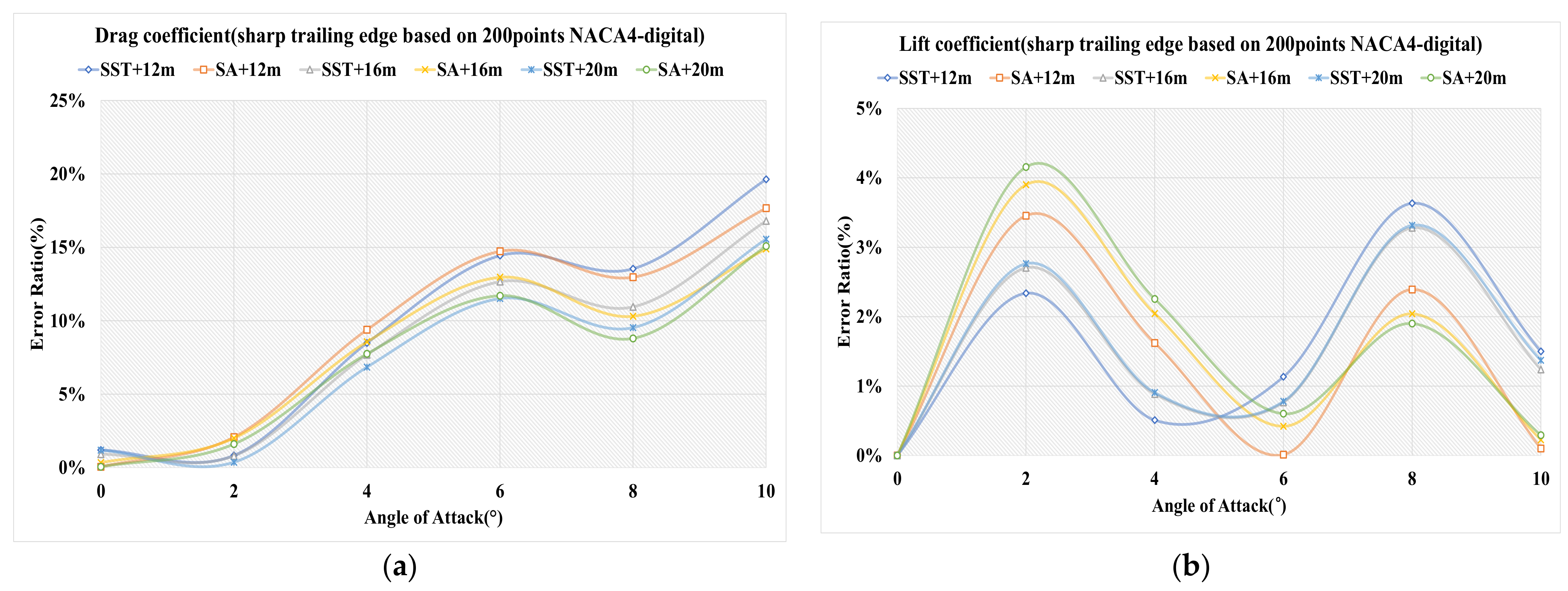
Figure 7 illustrates the error ratios of $C_d$ and $C_l$ between simulation data and experimental data, and Table 9 provides the corresponding mean error ratios under different AOA ranges. The optimal simulations were performed by SA+12 m, SST+20 m, SST+20 m, SST+20 m, SST+20 m, and SA+20 m and the relevant results are (0.05%, 0.00%), (0.78%, 1.38%), (2.80%, 1.22%), (4.98%, 1.11%), (5.89%, 1.55%), and (7.50%, 1.53%), respectively. At the range of (0°, 2°), although the $C_l$ of SST+12 is the smallest, the $C_d$ is relatively large. Considering the $C_d$ and $C_l$ comprehensively, the result of SST+20 m is optimum. At the range of (0°, 4°), despite SST+12 m obtaining the best result for $C_l$, the $C_d$ of SST+20 m is preferred. Due to the $C_d$ being a magnitude greater than the $C_l$, SST+20 m performs the best. At the range of (0°, 6°), similarly, the ideal result is obtained by SST+20 m. At the range of (0°, 10°), the result of SST+20 m is the same as that of SA+20 m. On the account of the variance of SA+20 m being lower than that of SST+20 m, SA+20 m behaves the best.

4.1.3. Sharp Trailing Edge Based on Definition Formula Applying 132 Points

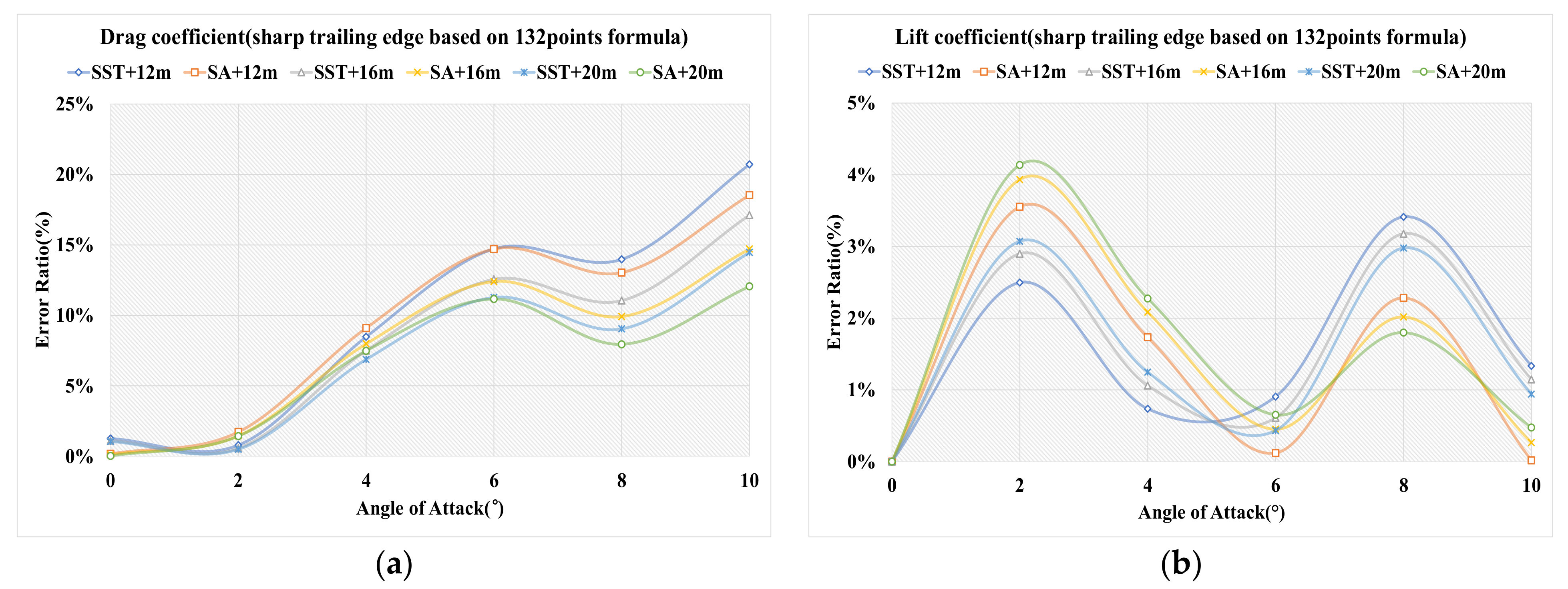
Figure 8 demonstrates the error ratios of $C_d$ and $C_l$ between simulation data and experiment data, and Table 10 provides the corresponding mean error ratios under different AOA ranges. The optimal results were (0.02%, 0.00%), (1.03%, 1.25%), (2.81%, 1.44%), (4.93%, 1.19%), (5.75%, 1.55%), and (6.68%, 1.56%), which were performed by SA+20 m, SST+12 m, SST+20 m, SST+20 m, SST+20 m, and SA+20 m, respectively. At the range of (0°, 2°), although the $C_d$ of SST+12 m is relatively large, the $C_l$ of that is the smallest. In a comprehensive comparison of the differences, SST+12 m behaves the best. At the range of (0°, 4°), SST+12 m obtains the minimum $C_l$, while the $C_d$ of SST+20 m is the smallest. Because the $C_d$ is a magnitude greater than the $C_l$, the performance of SST+20 m is preferred. At the range of (0°, 6°), similarly, the best result is obtained by SST+20 m.

4.1.4. Sharp Trailing Edge Based on Definition Formula Applying 200 Points

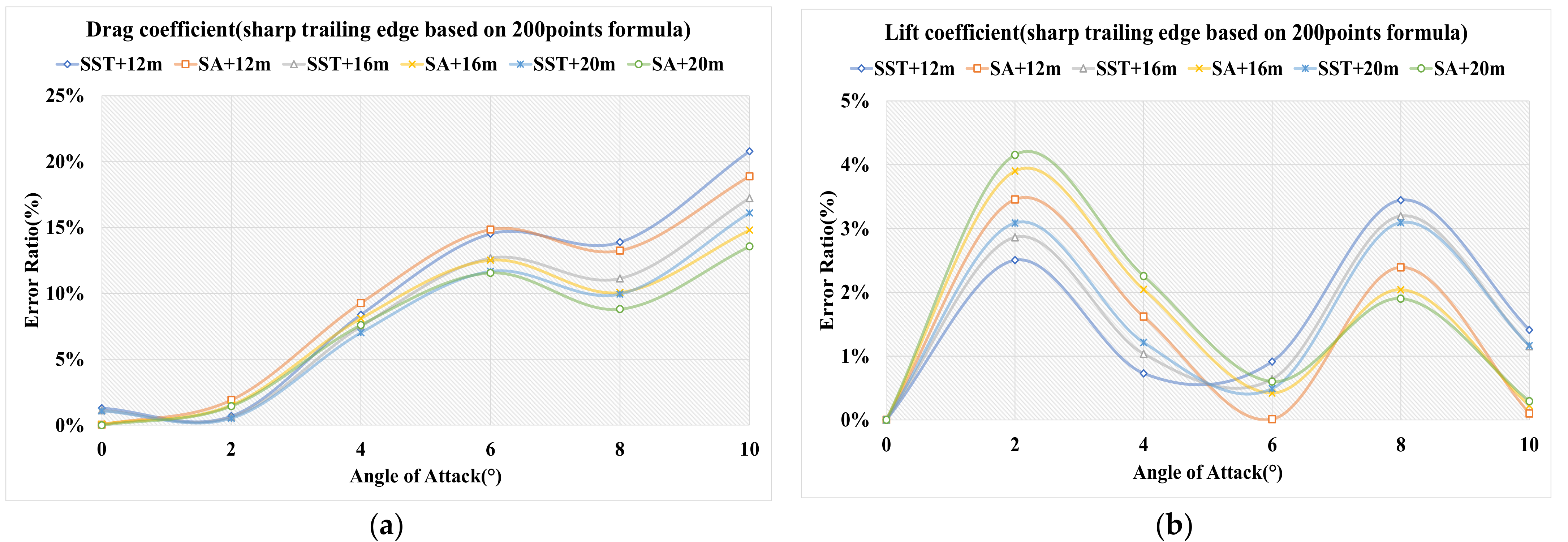
The error ratios of $C_d$ and $C_l$ between simulation data and experiment data are displayed in Figure 9, and Table 11 contains the related mean error ratios under different AOA ranges. The ideal results were achieved by SA+20 m, SST+12 m, SST+20 m, SST+20 m, SST+20 m, and SA+20 m, which were (0.00%, 0.00%), (0.99%, 1.25%), (2.88%, 1.43%), (5.07%, 1.20%), (6.05%, 1.58%), and (7.16%, 1.53%), respectively. At the range of (0°, 2°), SA+20 m has the lowest $C_d$, while the result of the $C_l$ is the largest. Considering the $C_d$ and $C_l$ comprehensively, the result of SST+12 m is optimum. At the range of (0°, 4°), although SST+12 m obtains the smallest result of $C_l$, the $C_d$ of SST+20 m is preferred. Due to the $C_d$ being a magnitude greater than the $C_l$, the best result is obtained by SST+20 m. Similarly, at the range of (0°, 6°), SST+20 m obtains the ideal result.

4.1.5. Sharp Trailing Edge Based on Definition Formula Applying 264 Points

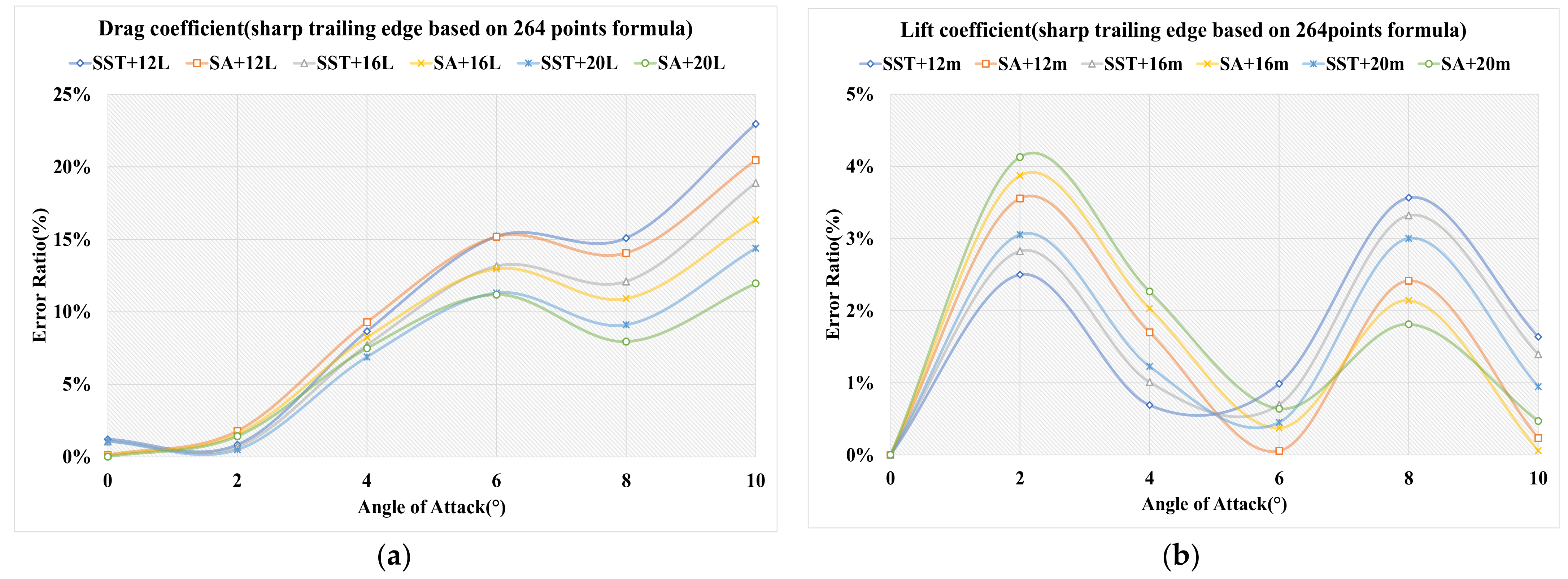
The error ratios of force coefficients between simulation data and experimental data are presented in Figure 10, and Table 12 shows the corresponding mean error ratios under different AOA ranges. SA+20 m, SST+12 m, SST+20 m, SST+20 m, SST+20 m, and SA+20 m afford the best results, which are (0.01%, 0.00%), (1.03%, 1.25%), (2.82%, 1.43%), (4.94%, 1.18%), (5.78%, 1.55%), and (6.67%, 1.55%), in order. At the range of (0°, 2°), although the $C_d$ of SA+20 m is the smallest, the $C_l$ is relatively large. Considering the $C_d$ and $C_l$ comprehensively, SST+12 m is preferred. At the range of (0°, 4°), similarly, the result of SST+20 m is the best. At the range of (0°, 10°), the $C_d$ of SA+20 m is the minimum, but the $C_l$ is not. Because the $C_d$ is a magnitude greater than the $C_l$, the optimal result is still achieved by SA+20 m.

4.1.6. Sharp Trailing Edge Based on Definition Formula Applying 400 Points

Figure 11 depicts the error ratios of force coefficients between simulation data and experimental data and under different AOA ranges; the related mean error ratios are presented in Table 13. The optimal simulations were executed by SA+16 m, SST+12 m, SST+20 m, SST+20 m, SST+20 m and SA+20 m and the results were (0.05%, 0.00%), (1.02%, 1.25%), (2.83%, 1.42%), (4.94%, 1.18%), (5.75%, 1.54%) and (6.67%, 1.55%), respectively. At the range of (0°, 2°), despite the result of SST+12 m being the same as that of SST+16 m, the variance of the former is superior to the latter. Therefore, SST+12 m behaves best. At the range of (0°, 4°), SST+12 m obtains the best result of $C_l$ and SST+20 m has the minimum $C_d$. Since the $C_d$ is a magnitude greater than the $C_l$, the performance of SST+20 m is preferred. At the range of (0°, 6°), similarly, the optimal result is obtained by SST+20 m.

4.2. Results of Far-Field Distances

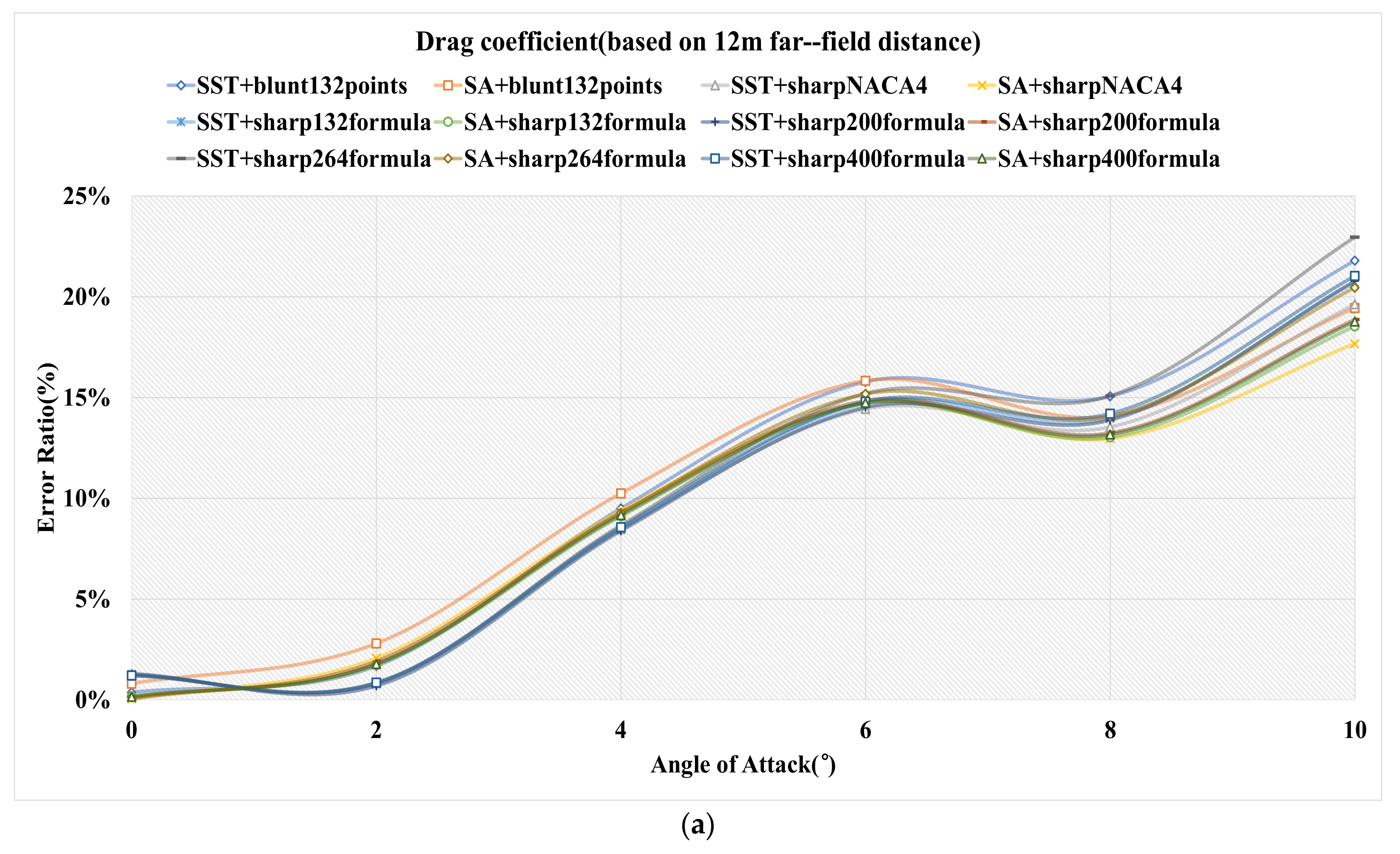
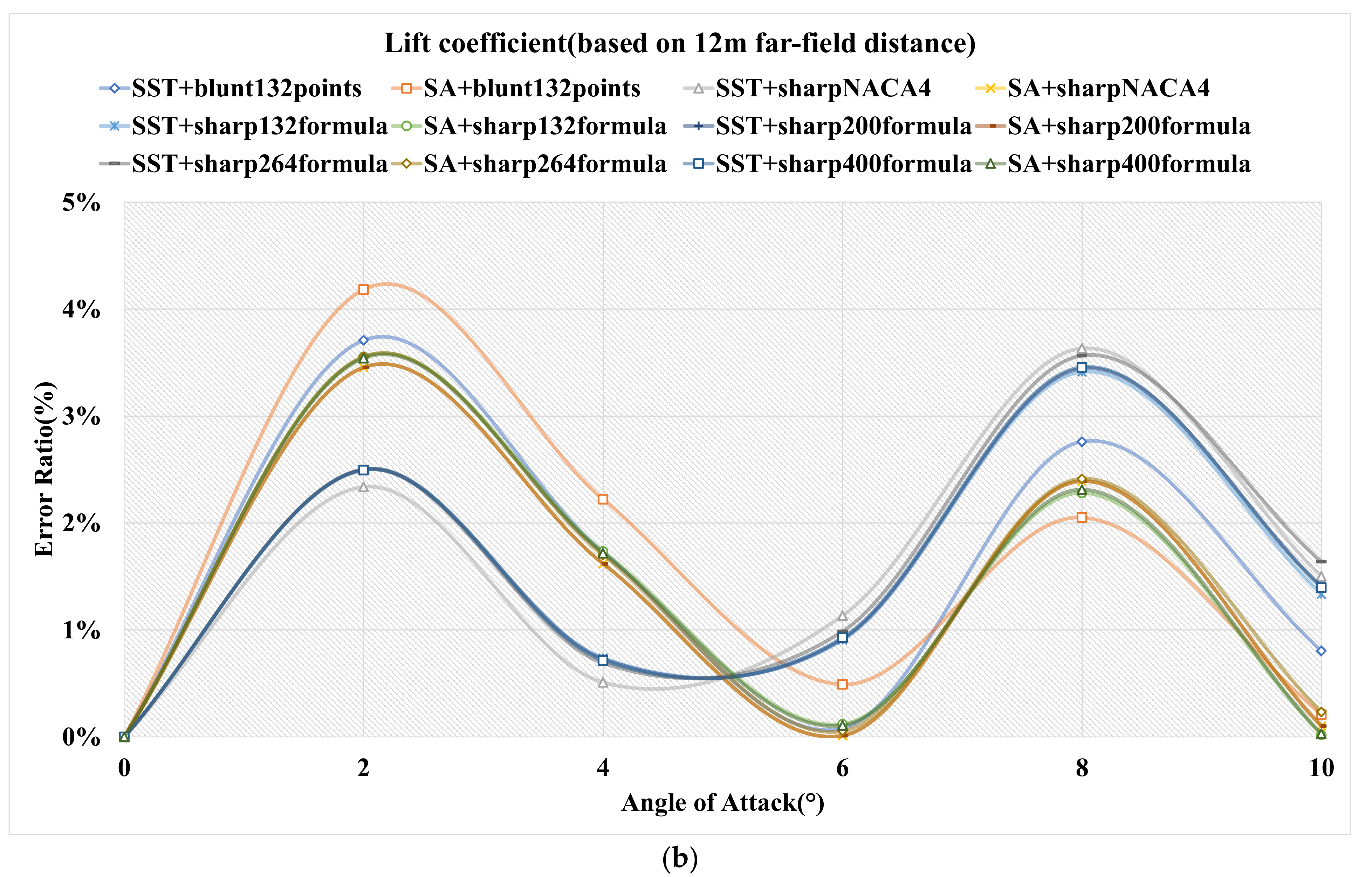
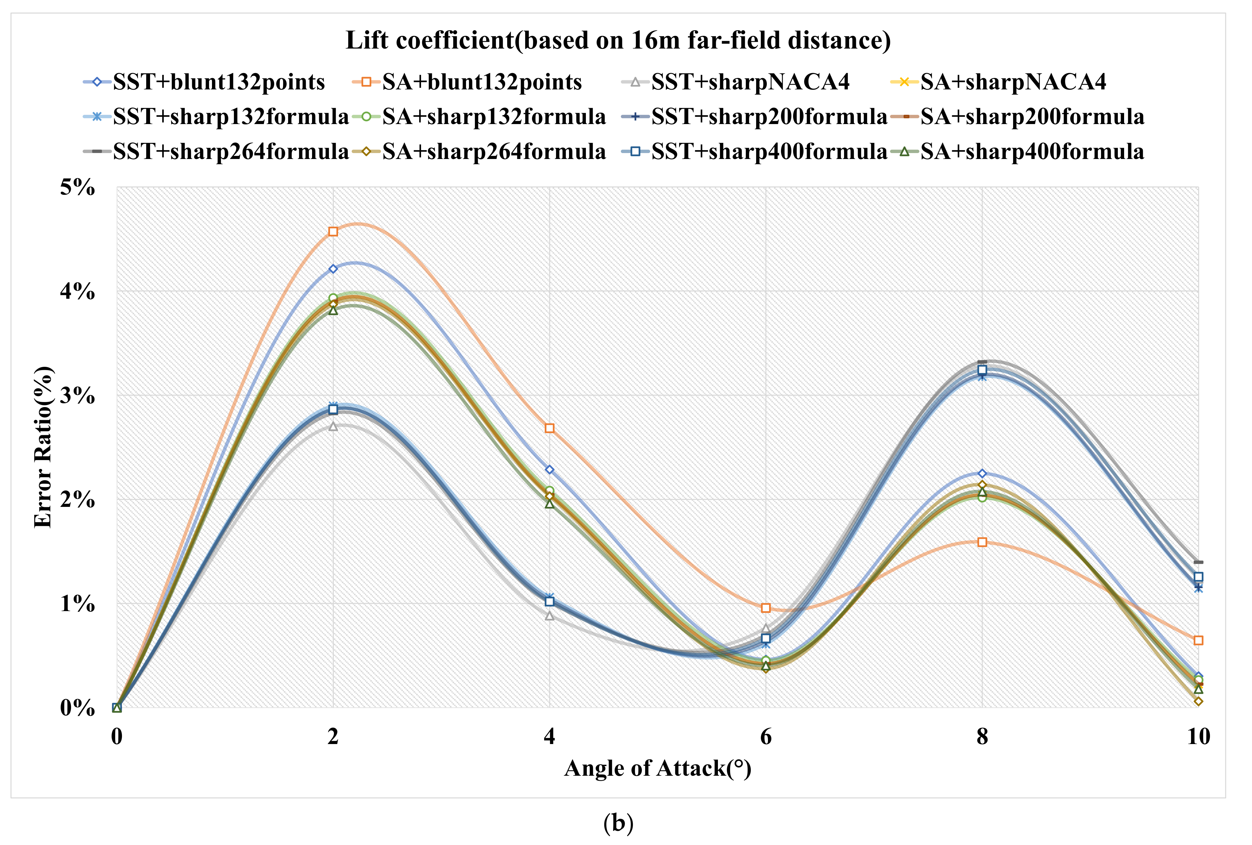
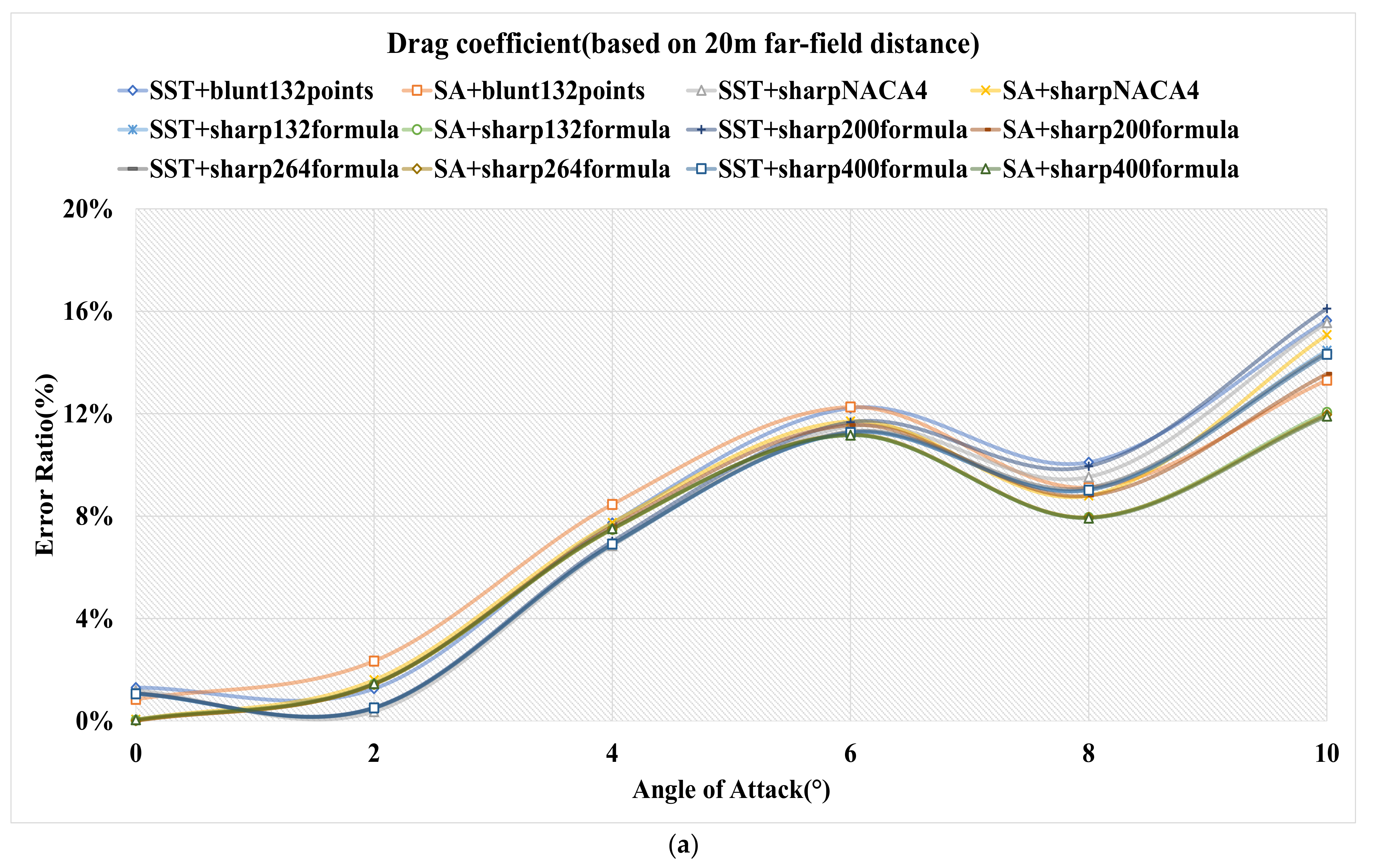
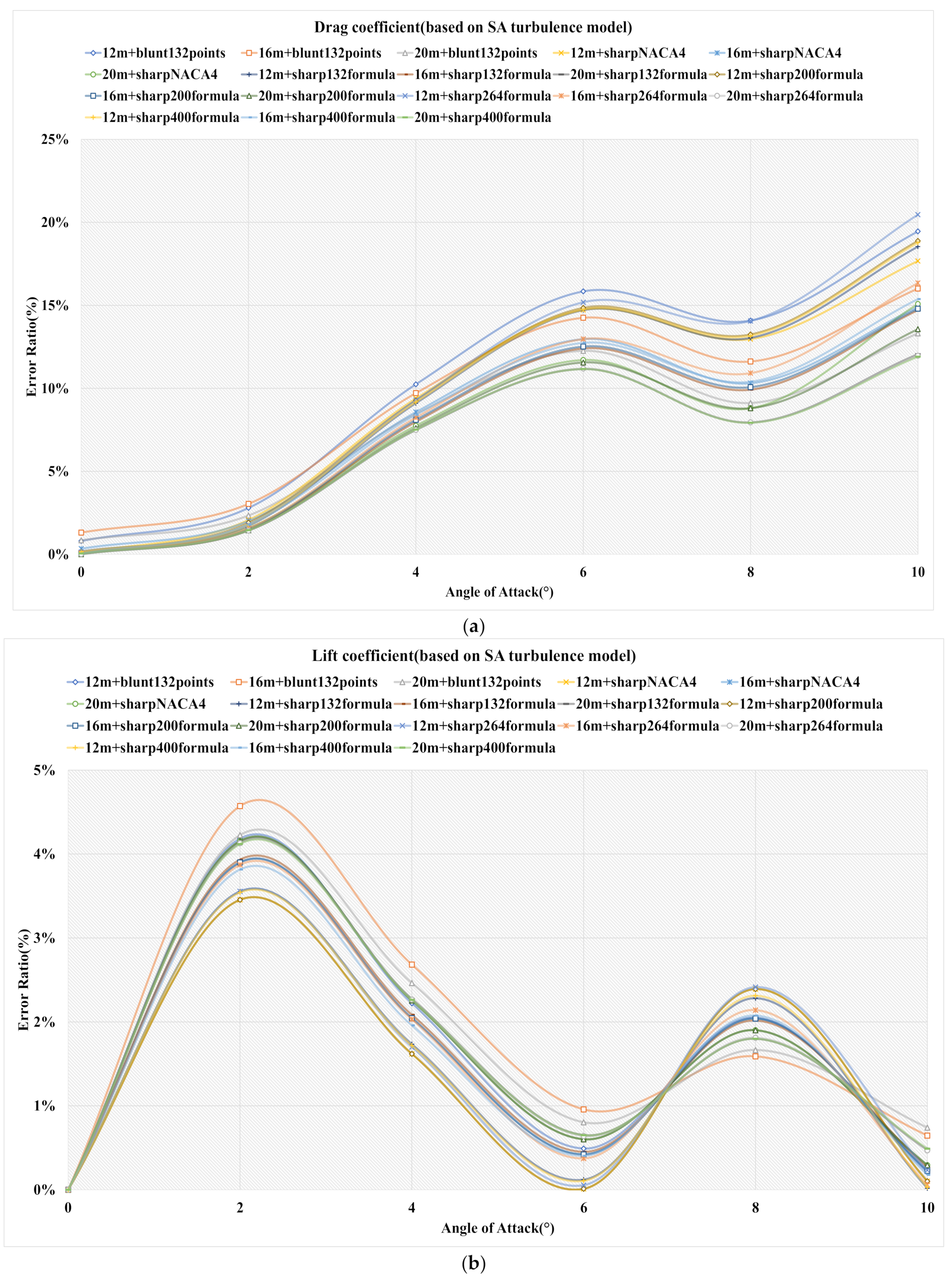
Based on the SST k-omega and Spalart–Allmaras turbulence models and six NACA0012 models, we made twelve simulation configurations: SST+blunt132points, SST+sharpNACA4, SST+sharp132formula, SST+sharp200formula, SST+sharp400formula, SA+blunt132points, SA+sharpNACA4, SA+sharp132formula, SA+sharp200formula, SST+sharp264formula, SA+sharp264formula, and SA+sharp400formula. Then, combined with the simulation parameters described in Table 4, twelve simulations were performed for each far-field distance. As in the previous section, the error ratios are illustrated in Figure 12, Figure 13 and Figure 14. The mean error ratios under different AOA ranges are contained in

Table 14. The mean error ratios of $C_d$ and $C_l$ of 12 m far-field distance.

Simulation Configurations	Range of AOA(°)
	$\mathbf{Mean} \mathbf{Error} \mathbf{Ratios} \mathbf{of} ({\mathit{C}}_{\mathit{d}}$$,{\mathit{C}}_{\mathit{l}})$
	(0°, 0°)	(0°, 2°)	(0°, 4°)	(0°, 6°)	(0°, 8°)	(0°, 10°)
SST+blunt	(0.37%, 0.00%)	(1.02%, 1.85%)	(3.85%, 1.81%)	(6.83%, 1.38%)	(8.48%, 1.66%)	(10.70%, 1.51%)
SST+NACA4	(1.19%, 0.00%)	(1.01%, 1.17%)	(3.50%, 0.95%)	(6.23%, 1.00%)	(7.69%, 1.52%)	(9.68%, 1.52%)
SST+132formula	(1.26%, 0.00%)	(1.03%, 1.25%)	(3.51%, 1.08%)	(6.31%, 1.04%)	(7.85%, 1.51%)	(9.99%, 1.48%)
SST+200formula	(1.30%, 0.00%)	(0.99%, 1.25%)	(3.46%, 1.08%)	(6.22%, 1.04%)	(7.75%, 1.52%)	(9.93%, 1.50%)
SST+264formula	(1.21%, 0.00%)	(1.02%, 1.25%)	(3.57%, 1.06%)	(6.48%, 1.04%)	(8.20%, 1.55%)	(10.66%, 1.56%)
SST+400formula	(1.21%, 0.00%)	(1.03%, 1.25%)	(3.54%, 1.07%)	(6.36%, 1.03%)	(7.93%, 1.52%)	(10.11%, 1.50%)
SA+blunt	(0.80%, 0.00%)	(1.80%, 2.09%)	(4.61%, 2.14%)	(7.42%, 1.72%)	(8.75%, 1.79%)	(10.54%, 1.53%)
SA+NACA4	(0.05%, 0.00%)	(1.06%, 1.73%)	(3.84%, 1.69%)	(6.56%, 1.27%)	(7.84%, 1.50%)	(9.48%, 1.26%)
SA+132formula	(0.18%, 0.00%)	(0.95%, 1.78%)	(3.67%, 1.76%)	(6.43%, 1.35%)	(7.75%, 1.54%)	(9.55%, 1.28%)
SA+200formula	(0.04%, 0.00%)	(0.98%, 1.73%)	(3.74%, 1.69%)	(6.52%, 1.27%)	(7.86%, 1.50%)	(9.70%, 1.26%)
SA+264formula	(0.13%, 0.00%)	(0.96%, 1.78%)	(3.73%, 1.75%)	(6.60%, 1.33%)	(8.09%, 1.54%)	(10.15%, 1.33%)
SA+400formula	(0.15%, 0.00%)	(0.96%, 1.77%)	(3.70%, 1.75%)	(6.46%, 1.34%)	(7.80%, 1.54%)	(9.63%, 1.28%)

,

Table 15. The mean error ratios of $C_d$ and $C_l$ of 16 m far-field distance.

Simulation Configurations	Range of AOA(°)
	$\mathbf{Mean} \mathbf{Error} \mathbf{Ratios} \mathbf{of} ({\mathit{C}}_{\mathit{d}}$$,{\mathit{C}}_{\mathit{l}})$
	(0°, 0°)	(0°, 2°)	(0°, 4°)	(0°, 6°)	(0°, 8°)	(0°, 10°)
SST+blunt	(0.21%, 0.00%)	(0.92%, 2.11%)	(3.50%, 2.17%)	(6.12%, 1.74%)	(7.39%, 1.84%)	(9.22%, 1.59%)
SST+NACA4	(0.91%, 0.00%)	(0.85%, 1.35%)	(3.13%, 1.20%)	(5.51%, 1.09%)	(6.60%, 1.53%)	(8.30%, 1.48%)
SST+132formula	(1.11%, 0.00%)	(0.84%, 1.45%)	(3.06%, 1.32%)	(5.43%, 1.14%)	(6.56%, 1.55%)	(8.32%, 1.48%)
SST+200formula	(1.12%, 0.00%)	(0.87%, 1.43%)	(3.08%, 1.30%)	(5.48%, 1.13%)	(6.61%, 1.55%)	(8.37%, 1.48%)
SST+264formula	(1.06%, 0.00%)	(0.83%, 1.94%)	(3.15%, 1.28%)	(5.65%, 1.13%)	(6.94%, 1.57%)	(8.93%, 1.54%)
SST+400formula	(1.04%, 0.00%)	(2.17%, 2.29%)	(3.12%, 1.29%)	(5.57%, 1.14%)	(6.76%, 1.56%)	(8.61%, 1.51%)
SA+blunt	(1.31%, 0.00%)	(1.17%, 1.95%)	(4.69%, 2.42%)	(7.08%, 2.05%)	(7.98%, 1.96%)	(9.32%, 1.74%)
SA+NACA4	(0.34%, 0.00%)	(0.78%, 1.97%)	(3.64%, 1.98%)	(5.97%, 1.59%)	(6.84%, 1.68%)	(8.18%, 1.44%)
SA+132formula	(0.11%, 0.00%)	(0.80%, 1.95%)	(3.18%, 2.01%)	(5.49%, 1.62%)	(6.37%, 1.70%)	(7.76%, 1.46%)
SA+200formula	(0.08%, 0.00%)	(0.92%, 1.91%)	(3.23%, 1.98%)	(5.55%, 1.59%)	(6.46%, 1.68%)	(7.85%, 1.44%)
SA+264formula	(0.09%, 0.00%)	(0.96%, 1.78%)	(3.30%, 1.97%)	(5.72%, 1.57%)	(6.76%, 1.68%)	(8.35%, 1.41%)
SA+400formula	(0.05%, 0.00%)	(0.88%, 1.41%)	(3.42%, 1.92%)	(5.75%, 1.54%)	(6.68%, 1.65%)	(8.13%, 1.41%)

and

Table 16. The mean error ratios of $C_d$ and $C_l$ of 20 m far-field distance.

Simulation Configurations	Range of AOA(°)
	$\mathbf{Mean} \mathbf{Error} \mathbf{Ratios} \mathbf{of} ({\mathit{C}}_{\mathit{d}}$$,{\mathit{C}}_{\mathit{l}})$
	(0°, 0°)	(0°, 2°)	(0°, 4°)	(0°, 6°)	(0°, 8°)	(0°, 10°)
SST+blunt	(1.31%, 0.00%)	(1.28%, 1.79%)	(3.43%, 1.75%)	(5.63%, 1.34%)	(6.52%, 1.61%)	(8.04%, 1.46%)
SST+NACA4	(1.19%, 0.00%)	(0.78%, 1.38%)	(2.80%, 1.22%)	(4.98%, 1.11%)	(5.89%, 1.55%)	(7.50%, 1.52%)
SST+132formula	(1.05%, 0.00%)	(0.78%, 1.54%)	(2.81%, 1.44%)	(4.93%, 1.19%)	(5.75%, 1.55%)	(7.20%, 1.45%)
SST+200formula	(1.08%, 0.00%)	(0.81%, 1.54%)	(2.88%, 1.43%)	(5.07%, 1.20%)	(6.05%, 1.58%)	(7.73%, 1.51%)
SST+264formula	(1.07%, 0.00%)	(0.79%, 1.53%)	(2.82%, 1.43%)	(4.94%, 1.18%)	(5.78%, 1.55%)	(7.21%, 1.45%)
SST+400formula	(1.06%, 0.00%)	(0.79%, 1.52%)	(2.83%, 1.42%)	(4.94%, 1.18%)	(5.75%, 1.54%)	(7.18%, 1.43%)
SA+blunt	(0.84%, 0.00%)	(1.59%, 2.11%)	(3.88%, 2.23%)	(5.97%, 1.87%)	(6.60%, 1.83%)	(7.72%, 1.65%)
SA+NACA4	(0.06%, 0.00%)	(0.83%, 2.08%)	(3.13%, 2.14%)	(5.28%, 1.75%)	(5.98%, 1.78%)	(7.50%, 1.53%)
SA+132formula	(0.02%, 0.00%)	(0.73%, 2.07%)	(2.98%, 2.14%)	(5.03%, 1.77%)	(5.61%, 1.77%)	(6.68%, 1.56%)
SA+200formula	(0.00%, 0.00%)	(0.72%, 2.08%)	(3.02%, 2.14%)	(5.15%, 1.75%)	(5.88%, 1.78%)	(7.16%, 1.53%)
SA+264formula	(0.01%, 0.00%)	(0.72%, 2.06%)	(2.98%, 2.13%)	(5.03%, 1.76%)	(5.61%, 1.77%)	(6.67%, 1.55%)
SA+400formula	(0.05%, 0.00%)	(0.75%, 2.06%)	(3.01%, 2.13%)	(5.05%, 1.76%)	(5.62%, 1.77%)	(6.67%, 1.55%)

and the corresponding optimal results and the simulation configurations are confirmed.

4.2.1. 12 m Far-Field Distance

Figure 12 shows the force coefficients error ratios, and Table 14 provides the corresponding mean errors under different AOA ranges. SA+200formula, SST+NACA4, SST+NACA4, SST+NACA4, SST+NACA4, and SA+NACA4 afforded the best performances, which were (0.04%, 0.00%), (1.01%, 1.17%), (3.50%, 0.95%), (6.23%, 1.00%), (7.69%, 1.52%) and (9.48%, 1.26%), respectively. At the range of (0°, 2°), although the $C_d$ of SST+132formula is the minimum, the $C_l$ is relatively large. Considering the $C_d$ and $C_l$ comprehensively, the result of SST+NACA4 is optimum. At the range of (0°, 4°), despite SST+200formula obtaining the smallest $C_d$, the $C_l$ of SST+NACA4 is preferred. Due to the $C_l$ being a magnitude greater than the $C_d$, the best result is accessed by SST+NACA4. Similarly, at the range of (0°, 6°), the optimal result is obtained by SST+NACA4.

4.2.2. 16 m Far-Field Distance

The error ratios of force coefficients are presented in Figure 13 and the related mean error ratios under different ranges of AOA are contained in Table 15. The optimal results are (0.05%, 0.00%), (0.85%, 1.35%), (3.13%, 1.20%), (5.43%, 1.14%), (6.37%, 1.70%) and (7.76%, 1.46%), in order, and the corresponding simulation configurations are SA+400formula, SST+NACA4, SST+NACA4, SST+132formula, SA+132formula, and SA+132formula. At the range of (0°, 2°), although the $C_d$ of SA+132formula is the minimum, the $C_l$ is relatively large. Considering the $C_d$ and $C_l$ comprehensively, SST+NACA4 is preferred. At the range of (0°, 4°), similarly, the result of SST+NACA4 is the best. At the range of (0°, 10°), SA+400formula obtains the minimum $C_l$ while the $C_d$ of SA+132formula is the best. Because the $C_d$ is a magnitude greater than the $C_l$, the optimal result is achieved by SA+132formula.

4.2.3. 20 m Far-Field Distance

Figure 14 demonstrates the error ratios of force coefficients and Table 16 illustrates the corresponding mean error ratios under different AOA ranges. The optimal simulations were performed by SA+200formula, SST+NACA4, SST+NACA4, SST+NACA4, SST+400formula and SA+400formula, in order, and the related results are (0.00%, 0.00%), (0.78%, 1.38%), (2.80%, 1.22%), (4.98%, 1.11%), (5.75%, 1.54%) and (6.67%, 1.55%). At the range of (0°, 2°), despite the $C_d$ of SA+264formula being the smallest, the $C_l$ is relatively large. Considering the $C_d$ and $C_l$ comprehensively, the result of SST+NACA4 is optimum. At the range of (0°, 8°), SA+132formula obtains the minimum $C_d$ while the $C_l$ of SST+400formula is the best. Due to the $C_l$ being a magnitude greater than the $C_d$, the optimal result is achieved by SST+400formula. Similarly, at the range of (0°, 10°), SA+400formula performs best.

4.3. Results of Turbulence Models

Based on the 12 m/16 m/20 m three far-field distances and six NACA0012 models, we made eighteen simulation configurations: 12 m+blunt132points, 12 m+sharpNACA4, 12 m+sharp132formula, 12 m+sharp200formula, 12 m+sharp264formula, 12 m+sharp400formula, 16 m+blunt132points, 16 m+sharpNACA4, 16 m+sharp132formula, 16 m+sharp200formula, 16 m+sharp264formula, 16 m+sharp400formula, 20 m+blunt132points, 20 m+sharpNACA4, 20 m+sharp132formula, 20 m+sharp200formula, 20 m+sharp264formula, and 20 m+sharp400formula. Then combined with the simulation parameters described in Table 4, for each turbulence model, eighteen simulations were performed. As in the previous sections, Figure 15 and Figure 16 depict the error ratios. By comparing the mean error ratios under different AOA ranges contained in

Table 17. The mean error ratios of $C_d$ and $C_l$ of SST k-omega turbulence model.

Simulation Configurations	Range of AOA(°)
	$\mathbf{Mean} \mathbf{Error} \mathbf{Ratios} \mathbf{of} ({\mathit{C}}_{\mathit{d}}$$,{\mathit{C}}_{\mathit{l}})$
	(0°, 0°)	(0°, 2°)	(0°, 4°)	(0°, 6°)	(0°, 8°)	(0°, 10°)
12 m+blunt	(0.37%, 0.00%)	(1.02%, 1.85%)	(3.85%, 1.81%)	(6.83%, 1.38%)	(8.48%, 1.66%)	(10.70%, 1.51%)
12 m+NACA4	(1.19%, 0.00%)	(1.01%, 1.17%)	(3.50%, 0.95%)	(6.23%, 1.00%)	(7.69%, 1.52%)	(9.68%, 1.52%)
12 m+132formula	(1.26%, 0.00%)	(1.03%, 1.25%)	(3.51%, 1.08%)	(6.31%, 1.04%)	(7.85%, 1.51%)	(9.99%, 1.48%)
12 m+200formula	(1.30%, 0.00%)	(0.99%, 1.25%)	(3.46%, 1.08%)	(6.22%, 1.04%)	(7.75%, 1.52%)	(9.93%, 1.50%)
12 m+264formula	(1.21%, 0.00%)	(1.02%, 1.25%)	(3.57%, 1.06%)	(6.48%, 1.04%)	(8.20%, 1.55%)	(10.66%, 1.56%)
12 m+400formula	(1.21%, 0.00%)	(1.03%, 1.25%)	(3.54%, 1.07%)	(6.36%, 1.03%)	(7.93%, 1.52%)	(10.11%, 1.50%)
16 m+blunt	(0.21%, 0.00%)	(0.92%, 2.11%)	(3.50%, 2.17%)	(6.12%, 1.74%)	(7.39%, 1.84%)	(9.22%, 1.59%)
16 m+NACA4	(0.91%, 0.00%)	(0.85%, 1.35%)	(3.13%, 1.20%)	(5.51%, 1.09%)	(6.60%, 1.53%)	(8.30%, 1.48%)
16 m+132formula	(1.11%, 0.00%)	(0.84%, 1.45%)	(3.06%, 1.32%)	(5.43%, 1.14%)	(6.56%, 1.55%)	(8.32%, 1.48%)
16 m+200formula	(1.12%, 0.00%)	(0.87%, 1.43%)	(3.08%, 1.30%)	(5.48%, 1.13%)	(6.61%, 1.55%)	(8.37%, 1.48%)
16 m+264formula	(1.06%, 0.00%)	(0.88%, 1.41%)	(3.15%, 1.28%)	(5.65%, 1.13%)	(6.94%, 1.57%)	(8.93%, 1.54%)
16 m+400formula	(1.04%, 0.00%)	(0.84%, 1.43%)	(3.12%, 1.29%)	(5.57%, 1.14%)	(6.76%, 1.56%)	(8.61%, 1.51%)
20 m+blunt	(1.30%, 0.00%)	(1.28%, 1.79%)	(3.43%, 1.75%)	(5.63%, 1.34%)	(6.52%, 1.61%)	(8.04%, 1.46%)
20 m+NACA4	(1.19%, 0.00%)	(0.78%, 1.38%)	(2.80%, 1.22%)	(4.98%, 1.11%)	(5.89%, 1.55%)	(7.50%, 1.52%)
20 m+132formula	(1.05%, 0.00%)	(0.78%, 1.54%)	(2.81%, 1.44%)	(4.93%, 1.19%)	(5.75%, 1.55%)	(7.20%, 1.45%)
20 m+200formula	(1.08%, 0.00%)	(0.81%, 1.54%)	(2.88%, 1.43%)	(5.07%, 1.20%)	(6.05%, 1.58%)	(7.73%, 1.51%)
20 m+264formula	(1.07%, 0.00%)	(0.79%, 1.53%)	(2.82%, 1.43%)	(4.94%, 1.18%)	(5.78%, 1.55%)	(7.21%, 1.45%)
20 m+400formula	(1.06%, 0.00%)	(0.79%, 1.52%)	(2.83%, 1.42%)	(4.94%, 1.18%)	(5.75%, 1.54%)	(7.18%, 1.43%)

and

Table 18. The mean error ratios of $C_d$ and $C_l$ of Spalart–Allmaras turbulence model.

Simulation Configurations	Range of AOA(°)
	$\mathbf{Mean} \mathbf{Error} \mathbf{Ratios} \mathbf{of} ({\mathit{C}}_{\mathit{d}}$$,{\mathit{C}}_{\mathit{l}})$
	(0°, 0°)	(0°, 2°)	(0°, 4°)	(0°, 6°)	(0°, 8°)	(0°, 10°)
12 m+blunt	(0.80%, 0.00%)	(1.80%, 2.09%)	(4.61%, 2.14%)	(7.42%, 1.72%)	(8.75%, 1.79%)	(10.54%, 1.53%)
12 m+NACA4	(0.05%, 0.00%)	(1.06%, 1.73%)	(3.84%, 1.69%)	(6.56%, 1.27%)	(7.84%, 1.50%)	(9.48%, 1.26%)
12 m+132formula	(0.18%, 0.00%)	(0.95%, 1.78%)	(3.67%, 1.76%)	(6.43%, 1.35%)	(7.75%, 1.54%)	(9.55%, 1.28%)
12 m+200formula	(0.04%, 0.00%)	(0.98%, 1.73%)	(3.74%, 1.69%)	(6.52%, 1.27%)	(7.86%, 1.50%)	(9.70%, 1.26%)
12 m+264formula	(0.13%, 0.00%)	(0.96%, 1.78%)	(3.73%, 1.75%)	(6.60%, 1.33%)	(8.09%, 1.54%)	(10.15%, 1.33%)
12 m+400formula	(0.15%, 0.00%)	(0.96%, 1.77%)	(3.70%, 1.75%)	(6.46%, 1.34%)	(7.80%, 1.54%)	(9.63%, 1.28%)
16 m+blunt	(1.31%, 0.00%)	(2.17%, 2.29%)	(4.69%, 2.42%)	(7.08%, 2.05%)	(7.98%, 1.96%)	(9.32%, 1.74%)
16 m+NACA4	(0.34%, 0.00%)	(1.17%, 1.95%)	(3.64%, 1.98%)	(5.97%, 1.59%)	(6.84%, 1.68%)	(8.18%, 1.44%)
16 m+132formula	(0.11%, 0.00%)	(0.78%, 1.97%)	(3.18%, 2.01%)	(5.49%, 1.62%)	(6.37%, 1.70%)	(7.76%, 1.46%)
16 m+200formula	(0.08%, 0.00%)	(0.80%, 1.95%)	(3.23%, 1.98%)	(5.55%, 1.59%)	(6.46%, 1.68%)	(7.85%, 1.44%)
16 m+264formula	(0.09%, 0.00%)	(0.83%, 1.94%)	(3.30%, 1.97%)	(5.72%, 1.57%)	(6.76%, 1.68%)	(8.35%, 1.41%)
16 m+400formula	(0.05%, 0.00%)	(0.92%, 1.91%)	(3.42%, 1.92%)	(5.75%, 1.54%)	(6.68%, 1.65%)	(8.13%, 1.41%)
20 m+blunt	(0.84%, 0.00%)	(1.59%, 2.11%)	(3.88%, 2.23%)	(5.97%, 1.87%)	(6.60%, 1.83%)	(7.72%, 1.65%)
20 m+NACA4	(0.06%, 0.00%)	(0.83%, 2.08%)	(3.13%, 2.14%)	(5.28%, 1.75%)	(5.98%, 1.78%)	(7.50%, 1.53%)
20 m+132formula	(0.02%, 0.00%)	(0.73%, 2.07%)	(2.98%, 2.14%)	(5.03%, 1.77%)	(5.61%, 1.77%)	(6.68%, 1.56%)
20 m+200formula	(0.00%, 0.00%)	(0.72%, 2.08%)	(3.02%, 2.14%)	(5.15%, 1.75%)	(5.88%, 1.78%)	(7.16%, 1.53%)
20 m+264formula	(0.01%, 0.00%)	(0.72%, 2.06%)	(2.98%, 2.13%)	(5.03%, 1.76%)	(5.61%, 1.77%)	(6.67%, 1.55%)
20 m+400formula	(0.05%, 0.00%)	(0.75%, 2.06%)	(3.01%, 2.13%)	(5.05%, 1.76%)	(5.62%, 1.77%)	(6.67%, 1.55%)

, we confirmed the corresponding optimal results and the simulation configurations.

4.3.1. SST k-Omega

The error ratios of force coefficients are presented in Figure 15 and the corresponding mean error ratios under different ranges of AOA are illustrated in Table 17. The models 16 m+blunt, 20 m+NACA4, 20 m+NACA4, 20 m+NACA4, 20 m+400formula, and 20 m+400formula provided the best performances, which were (0.21%, 0.00%), (0.78%, 1.38%), (2.80%, 1.22%), (4.98%, 1.11%), (5.75%, 1.54%), and (7.18%, 1.43%) respectively. At the range of (0°, 2°), although the $C_l$ of 12 m+NACA4 is the minimum, the $C_d$ is relatively big. Considering the $C_d$ and $C_l$ comprehensively, 20 m+NACA4 is preferred. Similarly, at the range of (0°, 4°), the result of 20 m+NACA4 is the best.

4.3.2. Spalart–Allmaras

Figure 16 depicts the force coefficients error ratios and Table 18 contains the mean error ratios under different AOA ranges. The optimal results are (0.00%, 0.00%), (0.98%, 1.73%), (2.98%, 2.13%), (5.03%, 1.76%), (5.61%, 1.77%), and (6.67%, 1.55%), and the corresponding simulation configurations are 20 m+200formula, 12 m+200formula, 20 m+264formula, 20 m+264formula, 20 m+132formula, and 20 m+400formula. At the range of (0°, 2°), despite the $C_l$ of 12 m+NACA4 being the same as that of 12 m+200formula, which is the smallest, the $C_d$ of those configurations is somewhat large. Considering the $C_d$ and $C_l$ comprehensively, 12 m+200formula is suggested. At the range of (0°, 4°), similarly, the result of 20 m+264formula is the best. At the range of (0°, 6°), the result of 20 m+132formula has the minimum $C_d$ while 20 m+264formula has the minimum $C_l$. Because the $C_l$ is a magnitude greater than the $C_d$, 20 m+264formula behaves best.

4.4. Discussion

Figure 17 presents the optimal total error ratios of the two trailing edge shapes and the corresponding calculation accuracy improvements. The sharp trailing edge performs better than the blunt trailing edge; in order, the accuracy improvements are 98.66%, 24.99%, 22.44%, 12.60%, 10.44%, and 12.25%. Therefore, the influence of the trailing edge shape on the calculation accuracy decreases as the AOA range increases, except at the range of (0°, 10°). For the sharp trailing edge adopting NACA4 and the definition formula, when the AOA ranges are (0°, 0°), (0°, 8°), and (0°, 10°), the definition formula is preferred and the accuracy improvements are 94.61%, 2.02%, and 8.97%, respectively. Conversely, when the AOA ranges are (0°, 2°), (0°, 4°), and (0°, 6°), the NACA4 is preferred. Therefore, the choice of NACA4 and formula depends on the studied range of AOA.

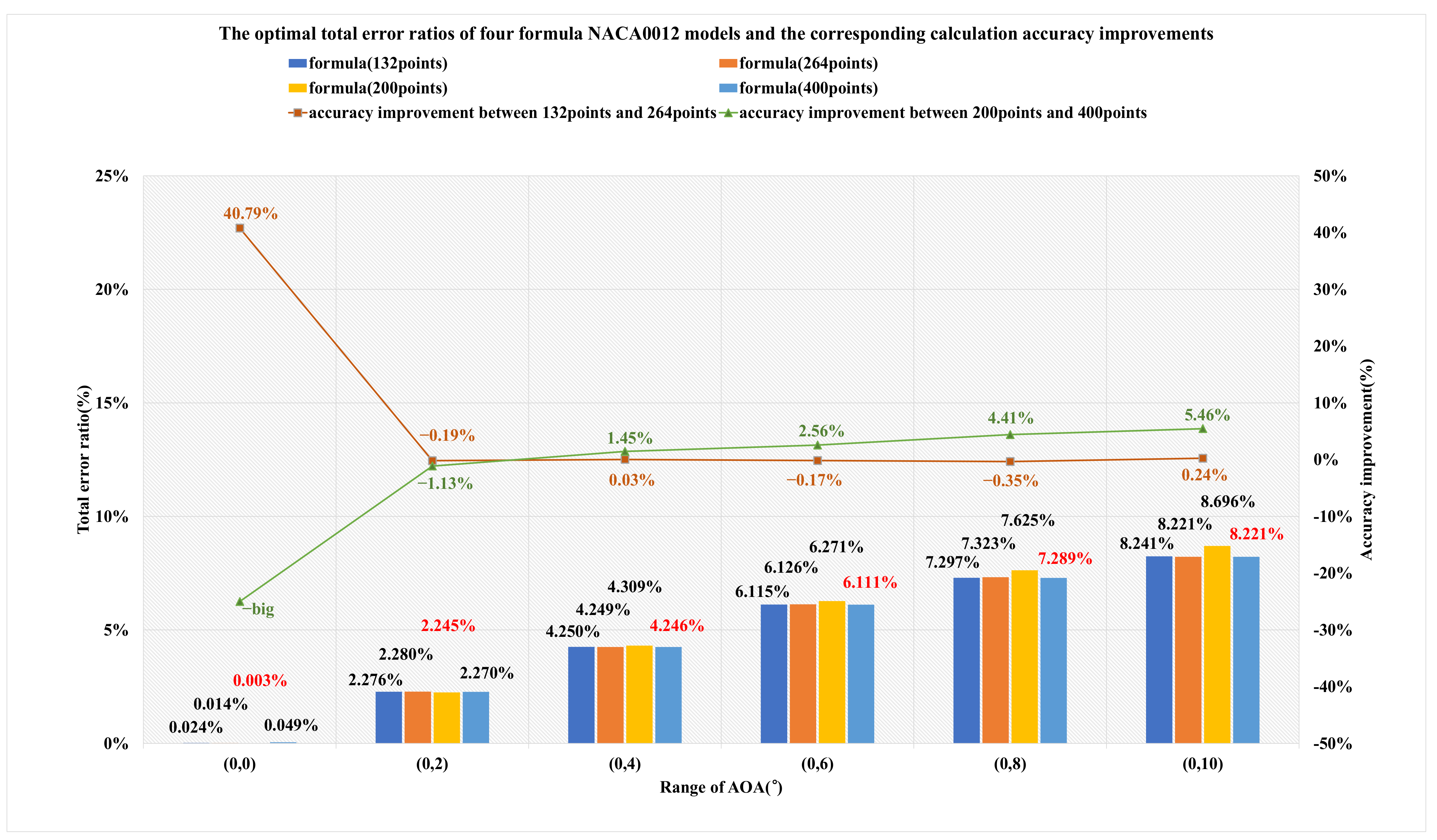
Furthermore, regarding the influence of the number of data points adopted in the definition formula on the simulation accuracy, Figure 18 presents the optimal total error ratios and the calculation accuracy improvements. From the 132 points provided by Airfoil Tools, when the data points doubled to 264 points, the accuracy improvements were 40.79%, −0.19%, 0.03%, −0.17%, −0.35%, and 0.24%, respectively. At the ranges of (0°, 0°), (0°, 4°), and (0°, 10°), the error ratios dropped but the declines in the latter two were very small. At the ranges of (0°, 2°), (0°, 6°), and (0°, 8°), the error ratios increased. Therefore, for the 132 points provided by Airfoil Tools, except at the range of (0°, 0°), the increase in the amount of data does not result in significant optimization of computational accuracy. For the 200 points provided by NACA4, as the data number doubled to 400 points, except at the ranges of (0°, 0°) and (0°, 2°), the error ratios dropped; the calculation accuracy improvements were 1.45%, 2.56%, 4.41%, and 5.46%. When the AOA range increased, the optimization effect brought by increasing the number of data points also increased. It should be noted that at the range of (0°, 0°), the optimal total error ratios are very small, at 0.003% and 0.049%, respectively. The ratio 0.049% still increased more than 100% compared to 0.003%, so the related accuracy improvement is described as “-big” in Figure 13. According to the best results under different AOA ranges, which are highlighted in red in Figure 13, the 200 points formula is preferred at the ranges of (0°, 0°) and (0°, 2°), while the 400 points formula is preferred at the ranges of (0°, 4°), (0°, 6°), (0°, 8°), and (0°, 10°). In short, the performance of the 200 points data is superior to that of the 132 points. For the 132 points, the number of data points is not directly correlated with calculation accuracy. For the 200 points, under the condition of a high AOA range, increasing the number of data points can improve the calculation accuracy.

Figure 19 presents the optimal total error ratios of three far-field distances and the corresponding calculation accuracy improvements. As the far-field distance rises from 12 L to 16 L, except at the ranges of (0°, 0°) and (0°, 2°), where the error ratios increase, the simulation accuracy increased by 2.78%, 9.01%, 12.44%, and 14.15%, respectively. Then, with the far-field distance further increasing to 20 L, compared with the 16 L far-field distance results, the error ratio decreased by 94.22%, 2.04%, 7.00%, 7.43%, 9.69%, and 10.85%. Compared with the results of 12 L far-field distance, the calculation accuracies of 20 L far-field distance increased by 93.50%, 0.88%, 9.58%, 15.77%, 20.92%, and 23.46%. The above results indicate that the key point is the degree of the far-field distance increases. When the AOA range is small ((0°, 0°), (0°, 2°)), boosting the far-field distance may not necessarily lead to an increment in simulation accuracy, but may lead to a drop. When the AOA range is large ((0°, 4°), (0°, 6°), (0°, 8°), (0°, 10°)), the greater the far-field distance, the better the simulation accuracy. As the range of the AOA grows larger, the improvement of calculation accuracy also increases, which means the degree of optimization brought by the increment of far-field distance has a positive correlation with the size of the AOA range. In conclusion, a far-field distance of 20 m is suggested.

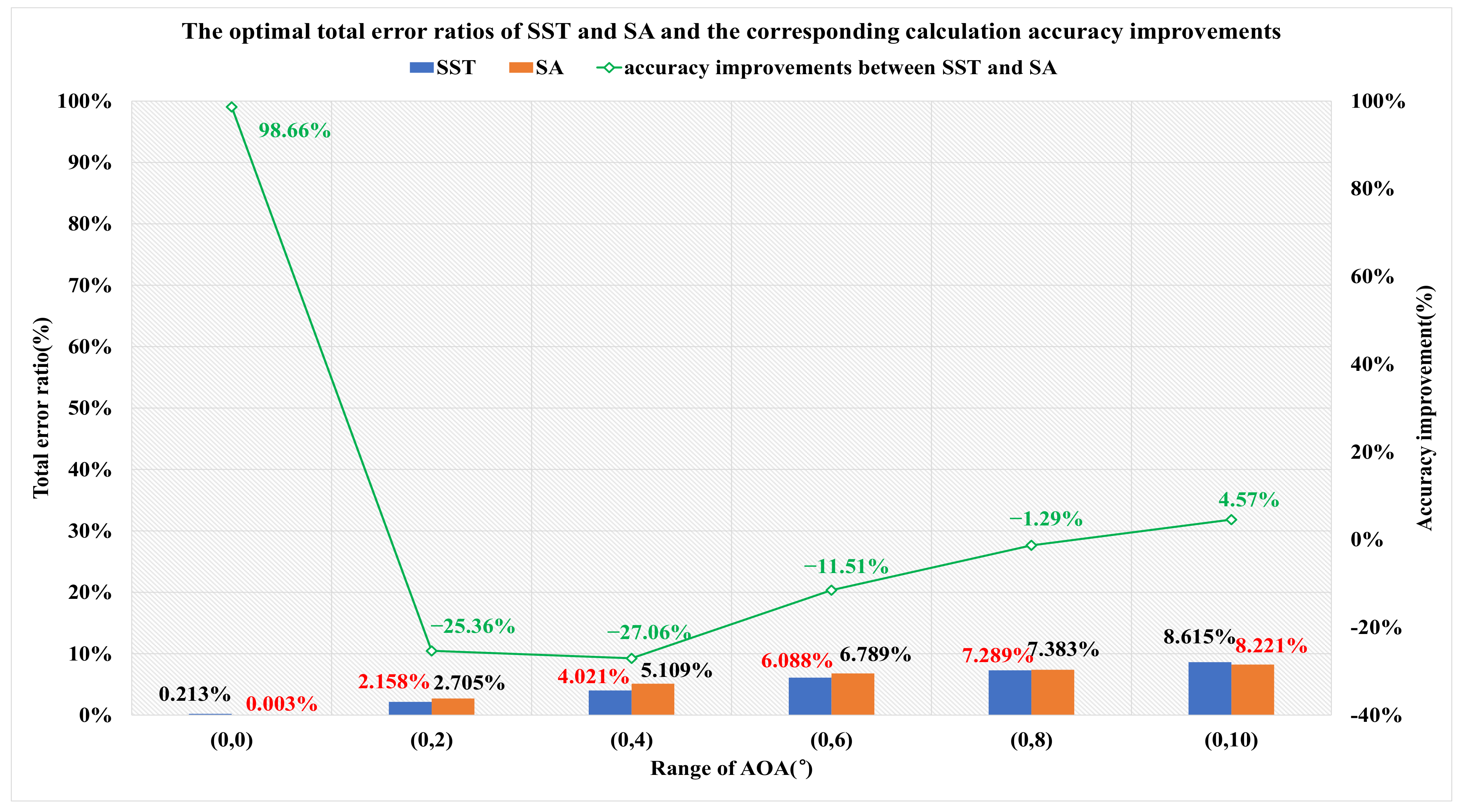
Figure 20 demonstrates the optimal total error ratios of SST k-omega and Spalart–Allmaras under different AOA ranges. At the ranges of (0°, 2°), (0°, 4°), (0°, 6°) and (0°, 8°), compared with the results of SST k-omega, the calculation accuracy changes with Spalart–Allmaras are −25.36%, −27.06%, −11.51% and −1.29%, which means SST k-omega performs better than Spalart–Allmaras. However, at the ranges of (0°, 0°) and (0°, 10°), Spalart–Allmaras behaves better than SST k-omega, with corresponding accuracy improvements of 98.66% and 4.57%. Therefore, when the AOA range is small (except (0°, 0°)), SST k-omega is preferred. However, when the AOA range increases, the performance difference between these two turbulence models decreases, and when the range increases to (0°, 10°), Spalart–Allmaras is preferred. In general, the range of AOA studied determines the chosen turbulence model.

Table 19. The optimal results and the corresponding simulation parameters.

Range of AOA(°)	Type of NACA0012 Model
	$\mathbf{The} \mathbf{Optimal} \mathbf{Mean} \mathbf{Error} \mathbf{Ratios} \mathbf{of} ({\mathit{C}}_{\mathit{d}}$
	Blunt Trailing Edge	Sharp Trailing Edge
		NACA4	Formula (132 Points)	Formula (200 Points)	Formula (264 Points)	Formula (400 Points)
(0°, 0°)	(0.21%, 0.00%)	(0.05%, 0.00%)	(0.02%, 0.00%)	(0.00%, 0.00%)	(0.01%, 0.00%)	(0.05%, 0.00%)
	SST+16 m	SA+12 m	SA+20 m	SA+20 m	SA+20 m	SA+16 m
(0°, 2°)	(1.02%, 1.85%)	(0.78%, 1.38%)	(1.03%, 1.25%)	(0.99%, 1.25%)	(1.03%, 1.25%)	(1.02%, 1.25%)
	SST+12 m	SST+20 m	SST+12 m	SST+12 m	SST+12 m	SST+12 m
(0°, 4°)	(3.43%, 1.75%)	(2.80%, 1.22%)	(2.81%, 1.44%)	(2.88%, 1.43%)	(2.82%, 1.43%)	(2.83%, 1.42%)
	SST+20 m	SST+20 m	SST+20 m	SST+20 m	SST+20 m	SST+20 m
(0°, 6°)	(5.63%, 1.34%)	(4.98%, 1.11%)	(4.93%, 1.19%)	(5.07%, 1.20%)	(4.94%, 1.18%)	(4.94%, 1.18%)
	SST+20 m	SST+20 m	SST+20 m	SST+20 m	SST+20 m	SST+20 m
(0°, 8°)	(6.52%, 1.61%)	(5.89%, 1.55%)	(5.75%, 1.55%)	(6.05%, 1.58%)	(5.78%, 1.55%)	(5.75%, 1.54%)
	SST+20 m	SST+20 m	SST+20 m	SST+20 m	SST+20 m	SST+20 m
(0°, 10°)	(7.72%, 1.65%)	(7.50%, 1.53%)	(6.68%, 1.56%)	(7.16%, 1.53%)	(6.67%, 1.55%)	(6.67%, 1.55%)
	SA+20 m	SA+20 m	SA+20 m	SA+20 m	SA+20 m	SA+20 m

gives the optimal mean error ratios and the corresponding simulation configurations based on the results of the previous three sections. In summary, if the AOA range is (0°, 0°), the sharp trailing edge based on the definition formula applying 200 points, combined with SA+20 m, achieves the optimal result, which is (0.00%, 0.00%). If the AOA ranges are (0°, 2°), (0°, 4°), and (0°, 6°), the sharp trailing edge based on 200 points NACA4-digital, combined with SST+20 m achieves the optimal results, which are (0.78%, 1.38%), (2.80%, 1.22%) and (4.98%, 1.11%). If the AOA range is (0°, 8°), the sharp trailing edge based on the definition formula applying 400 points, combined with SST+20 m, achieves the optimal result, which is (5.75%, 1.54%). If the range of AOA is (0°, 10°), the sharp trailing edge based on the definition formula applying 400 points, combined with SA+20 m, achieves the optimal result, which is (6.67%, 1.55%). If the applied trailing edge shape is blunt, the suggested corresponding simulation configurations are SST+16 m, SST+12 m, SST+20 m, SST+20 m, SST+20 m, and SA+20 m.

5. Conclusions

In this paper, based on the experimental data of Ref. [22], the effects of trailing edge shape and the corresponding modeling method, far-field distance, and turbulence model on the force coefficients under high Reynolds numbers are discussed. Section 2 introduces the applied modeling methods, grid divisions, turbulence models, and the numerical procedure. In Section 3, we confirm the appropriate grid strategy and the numerical method. The shape of the trailing edge and related modeling method dependencies, the far-field distance dependencies, and the turbulence model dependencies under six AOA ranges are expressed in Section 4. In particular, the number of data points adopted into the definition formula dependencies is discussed. Through systematic analysis, several conclusions can be drawn, as follows:

• nlike the choice of the trailing edge shape depending on the value of AOA under a lower Reynolds number, we should prioritize adopting the sharp trailing edge under a high Reynolds number. Therefore, the corresponding methods of NACA4 generator and the definition formula are suggested. The definition formula is preferred if the studied ranges are (0°, 0°), (0°, 8°), and (0°, 10°). If this is not the case, the NACA4 generator is preferred. It should be noted that a greater number of data points adopted into the definition formula does not neccesarily imply better performance. On the one hand, this may reqiore more computing resources. On the other hand, as described in Section 4.4, the improvement in calculation accuracy is limited, and accuracy may even be reduced.
• When plotting the computational domain of the airfoil external flow field, on the premise of sufficient computer resources, a far-field distance of 20 L is preferred. Although the increase of the far-field distance leads to the rise of the aspect ratio of the mesh quality, as long as it can be controlled within a reasonable range, which in this paper is smaller than 5000, the maximum far-field distance can bring the minimum simulation error ratio.
• The confirmation of the turbulence model depends on the AOA range with which one is concerned. The Spalart–Allmaras turbulence model performs better at AOA ranges of (0°, 0°) and (0°, 10°), while the SST k-omega performs better at AOA ranges of (0°, 2°), (0°, 4°), (0°, 6°), and (0°, 8°).
• In this paper, under the studied AOA ranges, the recommended simulation configurations are sharp trailing edge + 20 L far-field distance + SA/SST/SST/SST/SA, respectively, and the corresponding optimal results are (0.00%, 0.00%), (0.78%, 1.38%), (2.80%, 1.22%), (4.98%, 1.11%), (5.75%, 1.54%), and (6.67%, 1.55%).

References

1. Chen, F.; Liu, H.; Zhang, S. Time-adaptive loosely coupled analysis on fluid–thermal–structural behaviors of hypersonic wing structures under sustained aeroheating. Aerosp. Sci. Technol. 2018, 78, 620–636. [Google Scholar] [CrossRef]
2. Qu, F.; Kong, W.; Sun, D.; Bai, J. Shock-stable flux scheme for predicting aerodynamic heating load of hypersonic airliners. Sci. China Ser. G: Phys. Mech. Astron. 2019, 62, 984711. [Google Scholar] [CrossRef]
3. Lu, Y.; Guangming, Z. An Effective Simulation Scheme for Predicting the Aerodynamic Heat of a Scramjet-Propelled Vehicle. Appl. Sci. 2021, 11, 9344. [Google Scholar] [CrossRef]
4. 2D NACA 0012 Airfoil Validation Case. Available online: https://turbmodels.larc.nasa.gov/naca0012_val.html (accessed on 16 April 2021).
5. Qu, F.; Sun, D.; Bai, J.; Zuo, G.; Yan, C. Numerical investigation of blunt body’s heating load reduction with combination of spike and opposing jet. Int. J. Heat Mass Transf. 2018, 127, 7–15. [Google Scholar] [CrossRef]
6. Qu, F.; Chen, J.; Sun, D.; Bai, J.; Yan, C. A new all-speed flux scheme for the Euler equations. Comput. Math. Appl. 2019, 77, 1216–1231. [Google Scholar] [CrossRef]
7. Cook, C.; Balachandar, S.; Chung, J.; Vu-Quoc, L. A generalized Characteristic-Based Split projection method for Navier-Stokes with real fluids. Int. J. Heat Mass Transf. 2018, 124, 1045–1058. [Google Scholar] [CrossRef]
8. Sadikin, A.; Yunus, N.A.M.; Abd Hamid, S.A.; Ismail, A.; Salleh, S.; Ahmad, S.; Rahman, M.N.A.; Mahzan, S.; Ayop, S.S. A comparative study of turbulence models on aerodynamics characteristics of a NACA0012 airfoil. Int. J. Integr. Eng. 2018, 10, 134–137. [Google Scholar] [CrossRef] [Green Version]
9. Vassberg, J.C.; Jameson, A. In pursuit of grid convergence for two-dimensional Euler solutions. J. Aircr. 2010, 47, 1152–1166. [Google Scholar] [CrossRef] [Green Version]
10. Diskin, B.; Thomas, J.L.; Rumsey, C.L.; Schwoppe, A. Grid-convergence of Reynolds-averaged Navier-stokes solutions for benchmark flows in two dimensions. AIAA J. 2016, 54, 2563–2588. [Google Scholar] [CrossRef]
11. Lam, K.; Lin, Y.F.; Liu, Y.; Zou, L. Numerical Investigation of Flow Past a Wavy Airfoil. In Proceedings of the 2nd Interna-tional Conference on Mechanical and Aerospace Engineering (ICMAE 2011), Bangkok, Thailand, 29–31 July 2011; pp. 110–116. [Google Scholar]
12. Lin, Y.F.; Lam, K.; Zou, L.; Liu, Y. Numerical study of flows past airfoils with wavy surfaces. J. Fluids Struct. 2013, 36, 136–148. [Google Scholar] [CrossRef]
13. Matin, R.K.; Ghassemi, H.; Arzideh, M.H. Numerical study of the effect of geometrical changes on the aerodynamic performance. Int. J. Fluid Mech. Res. 2016, 43, 28–38. [Google Scholar] [CrossRef]
14. Devi, P.B.; Paulson, V.; Madhanraj, V.; Shah, D.A. Heat transfer and temperature effects on a dimpled NACA0012 airfoil with various angles of attack. Int. J. Ambient. Energy 2018, 39, 783–786. [Google Scholar] [CrossRef]
15. Li, Y.C.; Wang, J.J.; Zhang, P.F. Effects of Gurney flaps on a NACA0012 airfoil. Flow Turbul. Combust. 2002, 68, 27–39. [Google Scholar] [CrossRef]
16. Chao, D.D.; van Dam, C.P. Computational aerodynamic analysis of a blunt trailing-edge airfoil modification to the NREL phase VI rotor. Wind. Energy 2007, 10, 529–550. [Google Scholar] [CrossRef]
17. Grebert, A.; Bodart, J.; Joly, L. Investigation of wall-pressure fluctuations characteristics on a naca0012 airfoil with blunt trailing edge. In Proceedings of the 22nd AIAA/CEAS Aeroacoustics conference, Lyon, France, 30 May–1 June 2016. [Google Scholar]
18. Prigent, S.L.; Buxton, O.R.H.; Bruce, P.J.K. Wake of a lifting wing with cut-in sinusoidal trailing edges. AIAA J. 2017, 55, 1590–1601. [Google Scholar] [CrossRef]
19. Juntao, Z.; Zhongxi, H.; Zheng, G. Aerodynamic performance of configurations of two-dimension inflatable wings under high Reynolds number. J. Aerosp. Power 2017, 32, 657–665. (In Chinese) [Google Scholar]
20. Jha, S.K.; Gautam, U.; Pawar, P.; Narayanan, S. Investigations of Flow Phenomena Over a Flat Plate and NACA0012 Airfoil at High Angles of Attack. Iran. J. Sci. Technol. Trans. Mech. Eng. 2020, 44, 985–996. [Google Scholar] [CrossRef]
21. Arini, N.R.; Turnock, S.R.; Tan, M. A study of modified vertical axis tidal turbine to improve lift performance. Int. J. Electr. Energy 2016, 4, 37–41. [Google Scholar] [CrossRef] [Green Version]
22. Perrin, R.; Rattanasiri, P.; Lamballais, E.; Yooyen, S. Influence of the trailing edge shape on the aerodynamic characteristics of an airfoil at low Re number using RANS. IOP Conf. Ser. Mater. Sci. Eng. 2020, 886, 012021. [Google Scholar] [CrossRef]
23. Thomareis, N.; Papadakis, G. Effect of trailing edge shape on the separated flow characteristics around an airfoil at low Reynolds number: A numerical study. Phys. Fluids 2017, 29, 014101. [Google Scholar] [CrossRef] [Green Version]
24. Ansys, Inc. Ansys Fluent Theory Guide; ANSYS, Inc.: Canonsburg, PA, USA; p. 15317.
25. Smirnov, N.N.; Penyazkov, O.G.; Sevrouk, K.L.; Nikitin, V.F.; Stamov, L.I.; Tyurenkova, V.V. Tyurenkova, Detonation onset following shock wave focusing. Acta Astronaut. 2017, 135, 114–130. [Google Scholar] [CrossRef]
26. Menter, F.R. Two-equation eddy-viscosity turbulence models for engineering applications. AIAA J. 1994, 32, 1598–1605. [Google Scholar] [CrossRef] [Green Version]
27. Spalart, P.; Allmaras, S. A one-equation turbulence model for aerodynamic flows. Rech. Aerosp. 1994, 1, 5–21. [Google Scholar]
28. Jameson, A.; Schmidt, W.; Turkel, E. Numerical Solution of the Euler Equations by Finite Volume Methods Using Runge-Kutta Time-Stepping Schemes. Technical Report AIAA-81-1259. In Proceedings of the AIAA 14th Fluid and Plasma Dynamics Conference, Palo Alto, CA, USA, 23–25 June 1981. [Google Scholar]
29. Abbott, I.H.; von Doenhoff, A.E. Theory of Wing Sections; Dover Publications: New York, NY, USA, 1959. [Google Scholar]
30. Gregory, N.; O’Reilly, C.L. Low-Speed Aerodynamic Characteristics of NACA 0012 Aerofoil Sections, including the Effects of Upper-Surface Roughness Simulation Hoar Frost. Aerodynamic Division, N.P.L. Reports and Memoranda No. 3726 January, 1970. Available online: https://citeseerx.ist.psu.edu/viewdoc/download?doi=10.1.1.227.696&rep=rep1&type=pdf (accessed on 1 December 2021).
31. Ladson, C.L. Effects of Independent Variation of Mach and Reynolds Numbers on the Low-Speed Aerodynamic Characteristics of the NACA 0012 Airfoil Section. NASA TM: Washington, DC, USA, 1988; p. 4074. [Google Scholar]
32. Chorin, A.J. Numerical solution of the Navier-Stokes equations. Math. Comput. 1968, 22, 745. [Google Scholar] [CrossRef]
33. Barth, T.J.; Jespersen, D. The design and application of upwind schemes on unstructured meshes. In Proceedings of the AIAA 27th Aerospace Sciences Meeting, Reno, Nevada, 9–12 January 1989. Technical Report AIAA-89-0366. [Google Scholar]
Figure 1. (a) Six NACA0012 airfoil models; (b) close view of different models.
Applsci 12 00416 g001
Figure 2. (a) Grid division of the blunt trailing edge; (b) grid division of the sharp trailing edge.
Applsci 12 00416 g002
Figure 3. The TVR plot with y+ value of 0.5.
Applsci 12 00416 g003
Figure 4. (a) Computational domain; (b) close view of grids near the WALL region.
Applsci 12 00416 g004
Figure 5. (a) Close view of grids near the blunt trailing edge; (b) close view of grids near the sharp trailing edge.
Applsci 12 00416 g005
Figure 6. (a) Drag coefficient of blunt trailing edge based on Airfoil Tools; (b) lift coefficient of blunt trailing edge based on Airfoil Tools.
Applsci 12 00416 g006
Figure 7. (a) Drag coefficient of sharp trailing edge based on NACA 4-digital; (b) lift coefficient of sharp trailing edge based on NACA 4-digital.
Applsci 12 00416 g007
Figure 8. (a) Drag coefficient of sharp trailing edge based on 132 points formula; (b) lift coefficient of sharp trailing edge based on 132 points formula.
Applsci 12 00416 g008
Figure 9. (a) Drag coefficient of sharp trailing edge based on 200 points formula; (b) lift coefficient of sharp trailing edge based on 200 points formula.
Applsci 12 00416 g009
Figure 10. (a) Drag coefficient of sharp trailing edge based on 264 points formula; (b) lift coefficient of sharp trailing edge based on 264 points formula.
Applsci 12 00416 g010
Figure 11. (a) Drag coefficient of sharp trailing edge based on 400 points formula; (b) lift coefficient of sharp trailing edge based on 400 points formula.
Applsci 12 00416 g011
Figure 12. (a) Drag coefficient based on 12 m far-field distance; (b) lift coefficient based on 12 m far-field distance.
Applsci 12 00416 g012aApplsci 12 00416 g012b
Figure 13. (a) Drag coefficient based on 16 m far-field distance; (b) lift coefficient based on 16 m far-field distance.
Applsci 12 00416 g013aApplsci 12 00416 g013b
Figure 14. (a) Drag coefficient based on 20 m far-field distance; (b) lift coefficient based on 20 m far-field distance.
Applsci 12 00416 g014aApplsci 12 00416 g014b
Figure 15. (a) Drag coefficient based on SST k-omega turbulence model; (b) lift coefficient based on SST k-omega turbulence model.
Applsci 12 00416 g015
Figure 16. (a) Drag coefficient based on Spalart–Allmaras turbulence model; (b) lift coefficient based on Spalart–Allmaras turbulence model.
Applsci 12 00416 g016
Figure 17. The optimal total error ratios of two shapes trailing edge and the corresponding calculation accuracy improvements.
Applsci 12 00416 g017
Figure 18. The optimal total error ratios of four formula models and the corresponding calculation accuracy improvements.
Applsci 12 00416 g018
Figure 19. The optimal results of three far-field distances and the corresponding calculation accuracy improvements.
Applsci 12 00416 g019
Figure 20. The optimal total error ratios of turbulence models and the corresponding calculation accuracy improvements.
Applsci 12 00416 g020