Abstract
Nowadays material science involves powerful 3D imaging techniques such as X-ray computed tomography that generates high-resolution images of different structures. These methods are widely used to reveal information about the internal structure of geological cores; therefore, there is a need to develop modern approaches for quantitative analysis of the obtained images, their comparison, and classification. Topological persistence is a useful technique for characterizing the internal structure of 3D images. We show how persistent data analysis provides a useful tool for the classification of porous media structure from 3D images of hydrocarbon reservoirs obtained using computed tomography. We propose a methodology of 3D structure classification based on geometry-topology analysis via persistent homology.
1. Introduction
Complex structure analysis is a rapidly developing branch that comprises a broad spectrum of applications and modern data analysis methods. Such structures encompass many spatial features of various scales. Although many mathematical methods aim to describe such objects as of statistical origin, this work focuses on the approach based on topological data analysis. Statistical methods are often frequency-based and are well suited for capturing some regularities enclosed in the structure. However, when it comes to the analysis of significantly irregular formations (mostly naturally occurring), statistical methods may lack the ability to reflect the variety of spatial features present in such objects.
The main advantage of the topology-based approach is that it allows for the capture of the main structural features (such as tied parts, tunnels, and cavities) expressed through topological invariants, which appears to be extremely useful when describing such natural objects as core, soil samples, etc.
Application of computer tomography (CT) for studying the samples of hydrocarbon reservoirs has been steadily increasing in recent decades. CT was initially developed for obtaining medical scans [1,2] in the early 1970s. Soon it was proposed to use CT in geology, for instance for studying soil [3,4], meteorites [5], paleontology [6], geo-engineering [7], and sedimenthology [8]. CT can perform relatively rapid non-destructive scanning of the internal structure of solids at various scales.
The classification problem usually arises during studying porous media (for example, hydrocarbon reservoir samples). Solving it is urgent for combining results of varying survey methods or distinct samples into one dataset with the following statistical analysis. It is also essential for similar hydrocarbon reservoir matching (searching for the analogs).
Therefore, the classification problem appears during the following processes:
- 1.
- Getting a primary idea of what the object under study is;
- 2.
- Allocation of sufficiently homogeneous sampling zones for detailed study;
- 3.
- Extrapolation of structure and properties of a large volume, based on the research of a small part of it;
- 4.
- Grouping research results and their joint analysis;
- 5.
- Choosing the set of analogous samples, for example, for destructive methods of analysis.
Modern CT gives very detailed images (density maps) that can be counted as big data. Thus, an automated method for studying and classifying a large number of samples is needed, which would take into account the microstructure of the studied soil and at the same time be computationally simple and stable.
There are various approaches to the quantitative description of porous media using their 3D images. So, the internal structure of the pore space can be described using correlation functions, Minkowski functionals, or persistent homology.
Correlation functions allow one to describe the structure of three-dimensional porous media, efficiently compress and store structural information, and also provide a means to reconstruct the structure [9].
Minkowski functionals (MF) characterize the geometric and topological characteristics of a pore space [10]. MF were used to study the internal structure of sedimentary rocks [11,12], soils [13,14,15], ceramics [16], foams [17,18], and composite materials [19]. However, since the Minkowski functionals can be interpreted as the volume, area, and curvature of the surface of pore space and the Euler-Poincaré characteristic, they provide a single value measure by integrating over the surface of an object.
For a more detailed description of the topological structure of porous media, the full set of Betti numbers can be used [20,21] instead of the Euler-Poincaré characteristic (which is defined as the alternating sum of the Betti numbers). This approach was previously used to demonstrate differences in the topological structure of the pore space of soils extracted from different horizons [21]. A more detailed description of multiscale structures is possible using persistent homology.
Persistent homology (PH) is a tool of topological data analysis showing how the topological structure of data changes during the change on a scale of its perception. The theory of persistent data analysis started to develop at the end of the last century independently by three groups of scientists [22,23,24]. In 2002, the stability of persistent homology was shown [25], meaning that small changes in the source data lead to small changes in the barcodes of the corresponding homologies.
PH has found applications in material sciences [26], medical images analysis [27], bioscience [28], and geophysics [29]. This method has been applied to extract more detailed geometric information about amorphous solids compared to traditional methods [30]. Quantitative description based on tomographic images of the sphere packings [31,32,33] and natural rocks [34,35,36] was also performed using persistent homology.
Dynamic processes inside porous media, such as single-phase [37] and multiphase flows [38,39,40], mechanical deformations [40], or chemical dissolution [41,42], can also be quantitatively described using the PH. It should be noted that a similar approach can also be used for the analysis of dynamic processes into continuous media [43]. For example, a persistent homology approach for determining the trigger sites of crack initiation in iron ores has been presented [44].
The novel approach [45,46] based on the combination of persistent homology with machine learning techniques also demonstrates efficiency in the geometric description of media with complex internal structure.
We propose an automated porous media 3D image classification method based on its topological properties using persistent data analysis. It should be quick in terms of calculation computing power, stable, and allow for complex multiscale structure analysis.
The initial images of porous media obtained by CT scanning are in grayscale, and the voxel brightness is the X-ray density of the corresponding volume of the sample. Usually, porous medium models are described through the composition, properties, and distribution of the “phases” that form the object under study [33]. In the simplest and most common case, these phases are rock (solid mineral) and pore. This model is called binary. Therefore, in order to assign a voxel to one of the two phases, the image binarization procedure is performed, that is, the transition from grayscale to a black-and-white image. The binarization threshold is understood as the value by which the distinction is made. There are a number of methods for performing this procedure; in addition, the original image of the same object may slightly change (due to the noise signal) depending on the equipment used and the scanning mode. In this regard, the final binarized images of the same object may differ slightly—having an “error” relative to the “ideal” image. For this reason, the algorithms and methods used to analyze binary images must be robust, i.e., give a similar result with minor variations in the original image. This is extremely important for practical work with images of different quality; therefore, in this work, we consider the influence of the selected binarization threshold (allowing the error of choosing its optimal value in a number of cases) on the result and interpretation.
The literature describes various metrics that can be used for the classification and analysis of persistent diagrams obtained for solving the exact class of problems or studying some type of object. However, it is not known which of them are optimal for the objects under consideration: samples of porous media-natural reservoirs and what advantages and disadvantages each of them has. Therefore, a number of well-known metrics are tested to develop approaches, priorities, and restrictions in the subsequent analysis of similar objects.
The objectives of the work are:
- Develop natural porous media classification method based on topological properties analysis by persistent homologies with use of 3D X-ray density images;
- Develop and test the workflow on genuine core samples of several hydrocarbon reservoirs;
- Evaluate sensitivity to the input data (images) quality.
In the presented paper we will describe the workflow and samples we used. These samples have been obtained using micro-CT data since it provides an unprecedented level of detail of the inner porous structure. We will then name the software we used for the calculation of persistent diagrams and provide a brief overview of metrics for its comparing. After that, we provide obtained results, discuss them, and give a short conclusion.
2. Materials and Methods
2.1. Overview of Workflow
In this paper, the following algorithm for hydrocarbon reservoirs samples classification is proposed:
- 1.
- Automated (based on geometrical properties) or manual (based on expert’s decision) specifying the research area of the studied sample, creation of subsamples;
- 2.
- Subsample automated binarization;
- 3.
- Calculation of a signed Euclidean distance transform with [47];
- 4.
- Calculation of persistent diagrams and barcodes using python package “diamorse” [48], which implies computation using discrete Morse theory [49];
- 5.
- Calculation of pairwise distances between all the samples in all above-mentioned metrics;
- 6.
- Selection of one of the samples as a “base” sample, relative to which all the distances will be counted. Usually, as “base” a sample with a priori simplest structure is selected but if there is no such data all samples act as a “base” consequently, and more representative dataset is chosen after analysis;
- 7.
- Visualization of obtained distances between “base” sample and others as a 3D plot with axes representing distances in a certain homology (–);
- 8.
- Point cloud clustering and samples classification.
2.2. Used Samples
Four types of porous media were studied in this paper: sandstone Bentheimer, carbonate reservoir, and A and B sandstone hard-to-recover formations.
Bentheimer sandstone has been widely used for fluid flow studies and its properties are reported elsewhere [50,51].
2.3. Persistent Diagrams
We used the software package Diamorse [39,48] to compute the persistent homology signatures of data volumes. This package can process any two-phase image; for instance, these two phases can be two different formations or porous/grain phases. We performed only the last type of analysis. First, a signed Euclidean distance transform (SEDT) was calculated from the binary image [52]. This transform at each point reflects the Euclidean distance to the nearest pore/grain boundary; negative values represent the pore phase and positive values the grain phase.
2.4. Metrics for Comparing Diagrams
To compare persistent diagrams, we need a notion of distance between them. In this paper, we use three metrics for comparing diagrams: Bottleneck distance, Sliced Wasserstein distance, and Heat Kernel distance. Let us introduce briefly each metric.
2.4.1. Bottleneck Distance
Lets introduce a Bottleneck distance between two diagrams and as it proposed in [53]. We recall that persistent diagram is a multiset of pairs , where b refers to birth time and d to dead time.
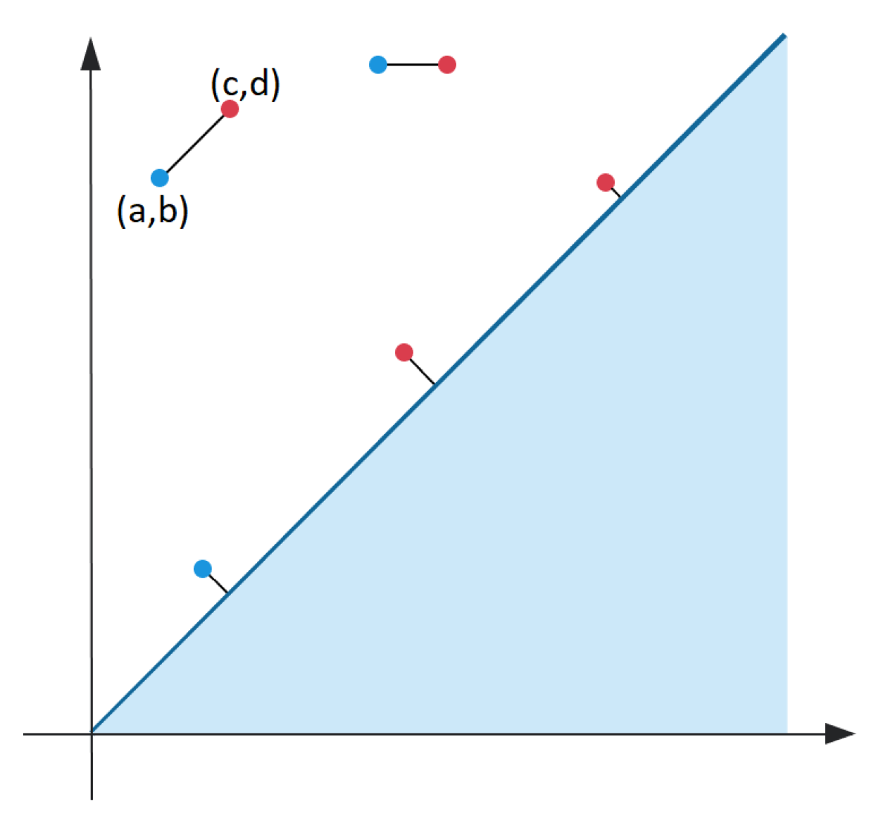
A matching between diagrams and pairs each point belonging to with a point in or some point on the diagonal line and vice versa for . See Figure 1 for illustration. In this definition we use the metric to get the distance between point and its matched point :
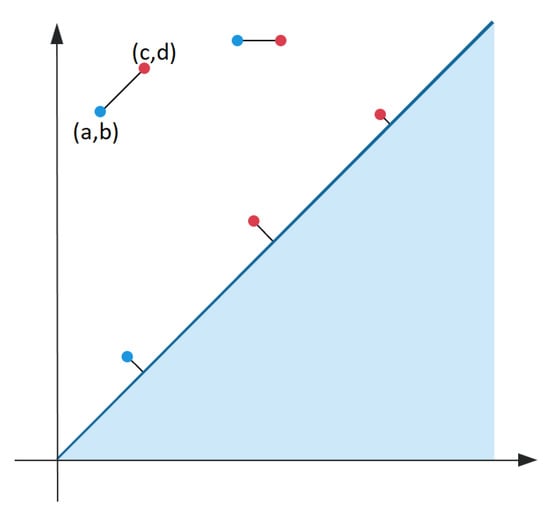
Figure 1.
A matching between points in (plotted in blue) and (plotted in red). Some points of each diagram are matched to the diagonal.
Let the size of a matching refer to the supremum of the distance between matched points. We are looking for matching with the smallest size among all possible matchings.
Definition 1.
The Bottleneck distance between persistence diagrams and is
where the supremum is taken over all matched points χ and the infinum is taken over all matchings η.
2.4.2. Sliced Wasserstein Distance
The Wasserstein distance [54,55] is a distance between probability measures. We will focus on a variant of that distance: the 1-Wasserstein distance for non-negative, not necessarily normalized, measures on the real line [56]. Let and be two non-negative measures on the real line such that their integrals on a real number line are equal. Then:
where —sets of measures on a plane with margin distributions and . This is the generic Kantorovich formulation of optimal transport, which is simply generalized to other cost functions and spaces, the modification being that we consider an unnormalized mass by reflecting it directly in the set
Then let us consider constructing a Sliced Wasserstein distance. Let there be a vector , . Let be a line , and is an orthogonal projection operator at . —persistent diagrams and and —“side view” of diagram point cloud, where —an orthogonal projection operator on the diagonal. Similar equations could be written for . Then, Sliced Wasserstein distance between could be defined as follows:
where is the unit sphere.
Therefore, to get the Sliced Wasserstein distance, the projections on straight lines passing through the origin were taken and the ordinary Wasserstein distance was calculated for all the angles of the line.
2.4.3. Heat Kernel Distance
Let us provide a definition of kernel function taken from [57]. Given a set , a function is a kernel if there exists a Hilbert space , called feature space, and a map , called feature map, such that . Equivalently, k is a kernel if it is symmetric and positive definite. Kernels allow for the application of machine learning algorithms operating on a Hilbert space to be applied to more general settings, such as strings, graphs, or, in our case, persistence diagrams. A kernel induces a pseudometric on , which is the distance in the feature space. We call the kernel k stable w.r.t. a metric d on if there is a constant such that .
Now let us get to the definition of the Heat Kernel distance. Let denote the space above the diagonal, and let denote a Dirac delta centered at the point p. For a given persistence diagram D, we now consider the solution of the partial differential equation:
The solution can be obtained as follows:
Let denote persistence diagrams. Using this closed form solution of u, we can derive a simple expression for evaluating the kernel explicitly:
where and are points of diagrams and accordingly, mirrored at the diagonal. The additional scale parameter is the dispersion parameter in Gaussian kernel. Finally, for Heat Kernel distance we have:
3. Results
We used the proposed algorithm to find and plot the distances between persistent diagrams of selected samples:
An—the A Formation type (A), n refers to different binarization threshold and resolution as follows:
- A1—resolution is 16.5 m/pixel, binarization threshold (t) = 103
- A2—16.5 m/px, t = 113
- A3—16.5 m/px, t = 123
- A4—16.5 m/px, t = 133
- A5—16.5 m/px, t = 143
- A6—33 m/px, t = 113
S—Sandstone Bentheimer (Sandstone), 20 m/px, different subsamples with same threshold;
C—carbonate rock (Carbonate), 20 m/px, different subsamples with same threshold;
T—T formations, 25 m/px, different subsamples with same threshold.
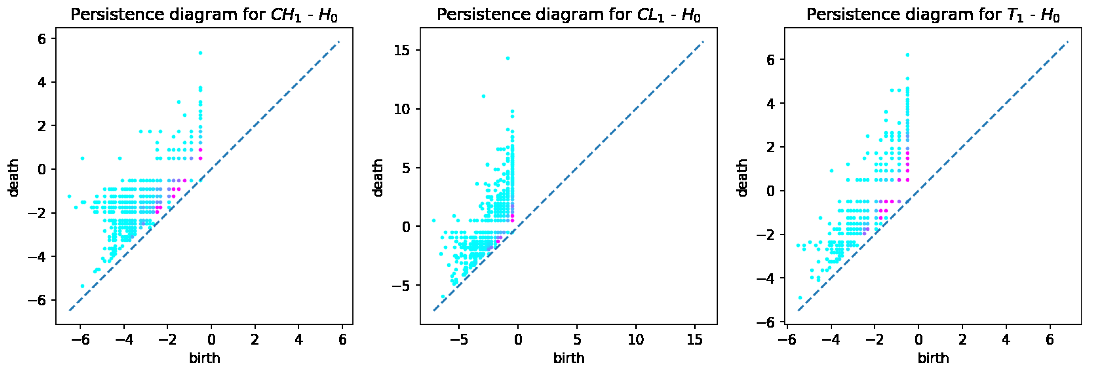
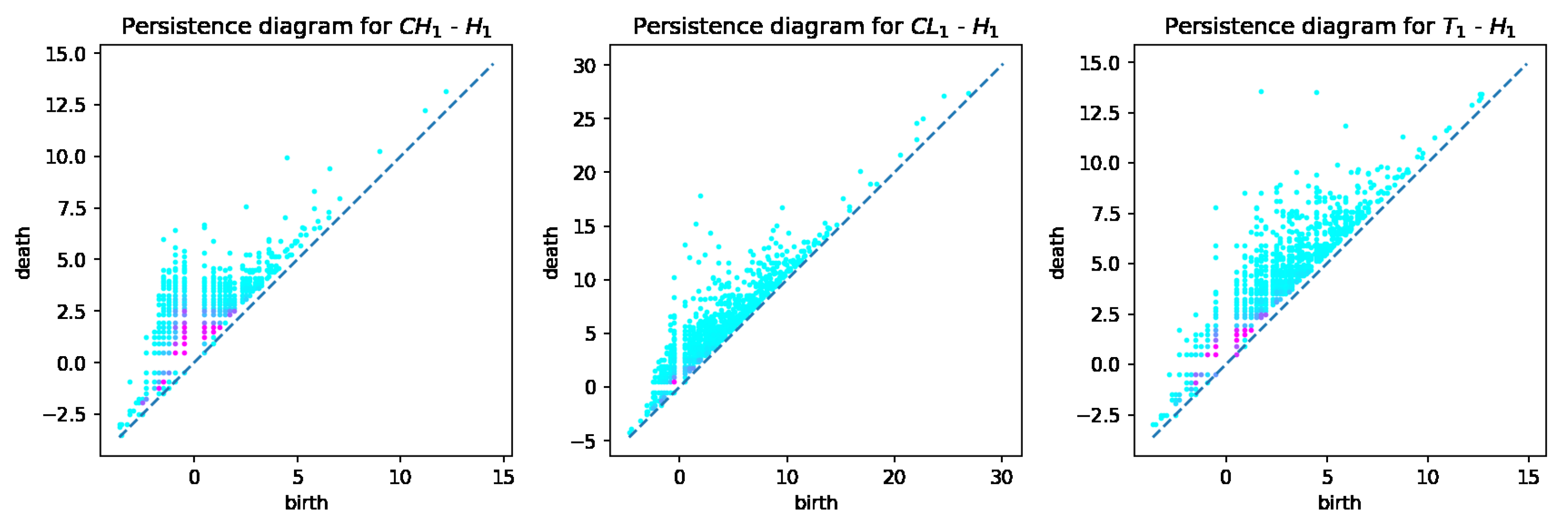
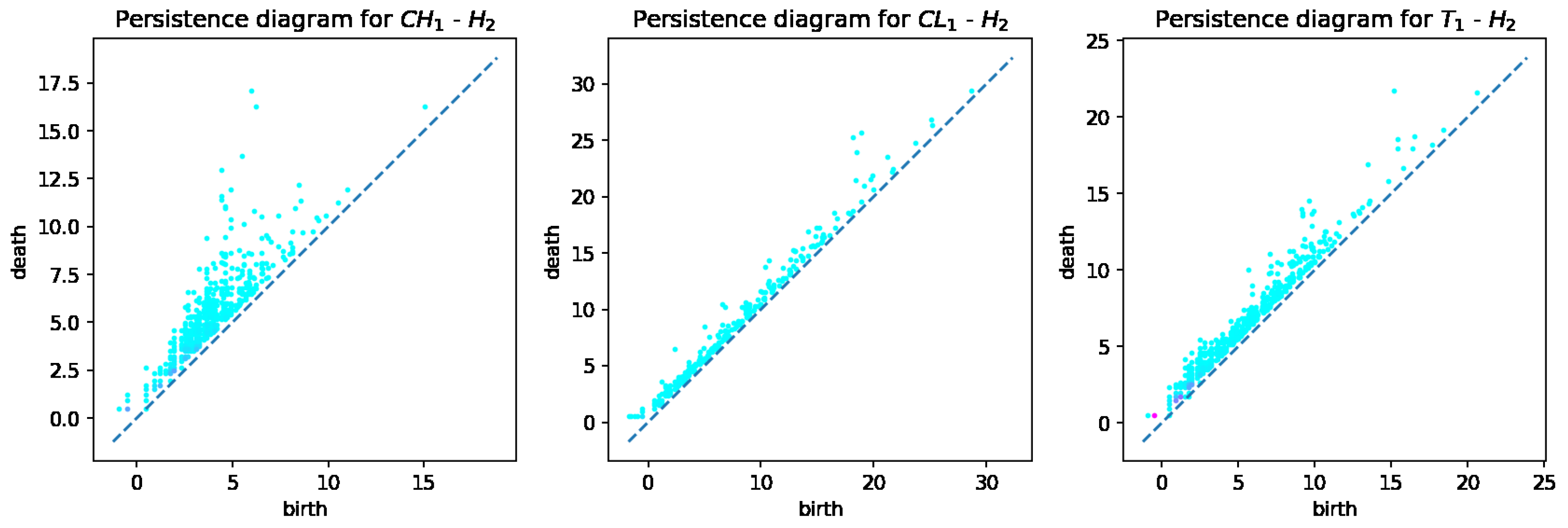
From the computed persistent diagrams for , we can see that point clouds for CH and T samples (Figure 2) are on average closer to the diagonal line than that of the CL sample. That means CL has more topologically significant connected components (more long-living topological features) and was formed from bigger fractions. As for diagrams in Figure 3, we can see that point cloud for CH sample is more concentrated along with the diagonal than those of CL and T samples. That means CL and T samples have on average wider tunnels passing through them than CH samples. From diagrams in Figure 4, we can note that the cloud point for the CH sample has more distance from the diagonal line points. That means the CH sample has on average more enclosed cavities than CL and T samples.
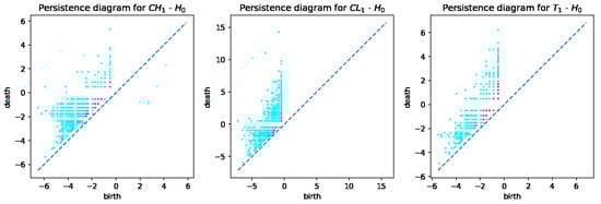
Figure 2.
persistent diagrams for CH, CL, and T samples.
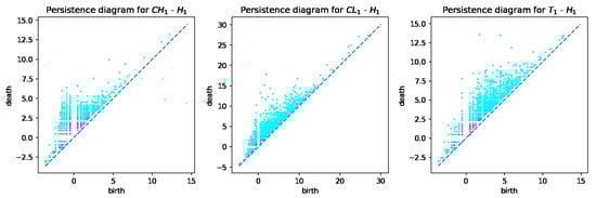
Figure 3.
persistent diagrams for CH, CL, and T samples.
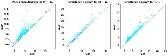
Figure 4.
persistent diagrams for CH, CL, and T samples.
Then we calculated distances between the “base” sample and each other. As the “base” sample we chose .
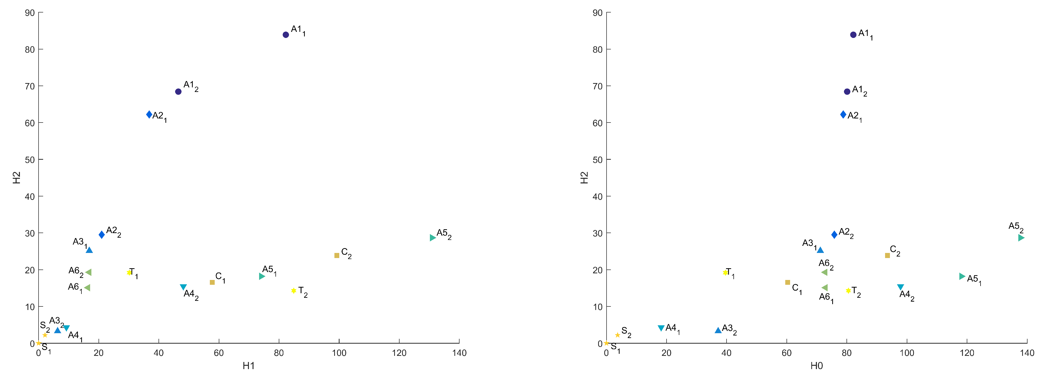
Figure A1 presents distances between “base” sample and others in Bottleneck metric in the 3D plot, as we described above, and in Figure 5 are presented projections of this plot on – and – planes. We can see that samples are not well clustered in this metric.
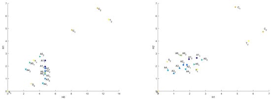
Figure 5.
Common distances in Bottleneck metric in – and – coordinates.
Figure 6 and Figure 7 present distances between “base” sample and others in Heat Kernel metric, as well as projections of this plot on –, –, and – planes.
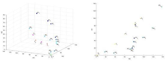
Figure 6.
Common distances in Heat Kernel metric in 3D and – coordinates.

Figure 7.
Common distances in Heat Kernel metric in – and – coordinates.
Figure A1 presents distances between “base” sample and others in Sliced Wasserstein metric; in Figure 8 are presented projections of this plot on – and – planes.

Figure 8.
Common distances in Sliced Wasserstein metric in – and – coordinates.
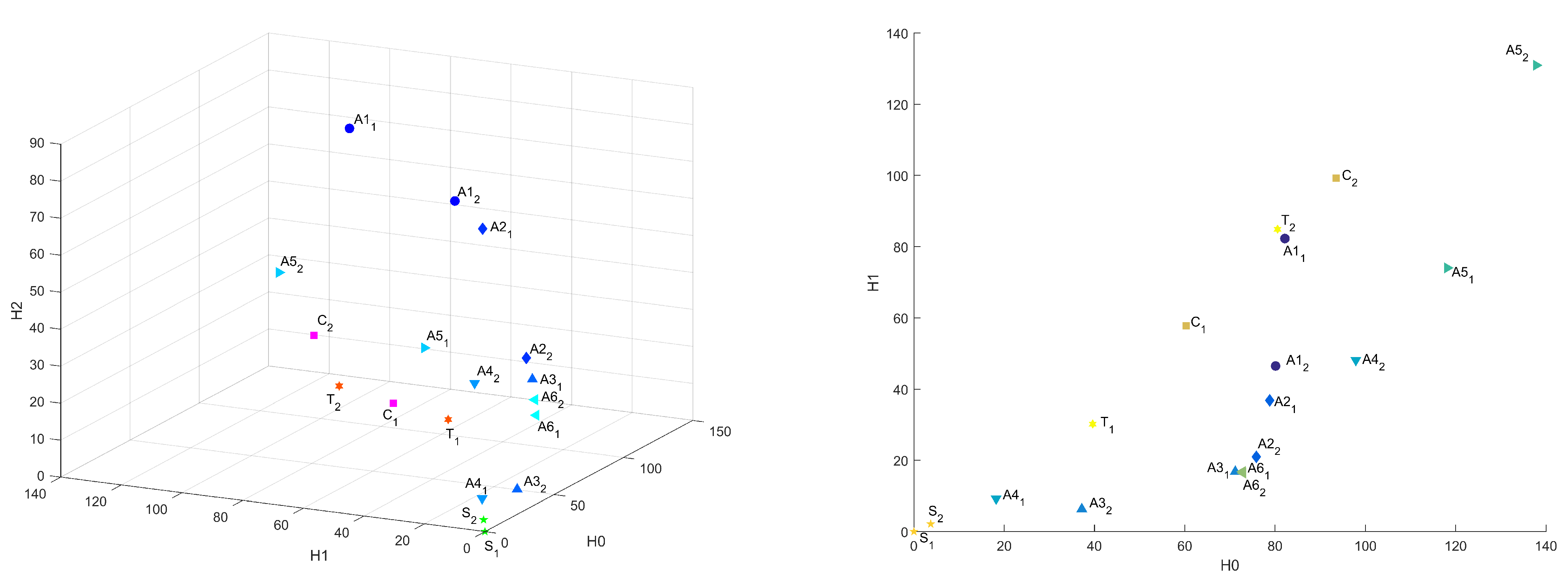
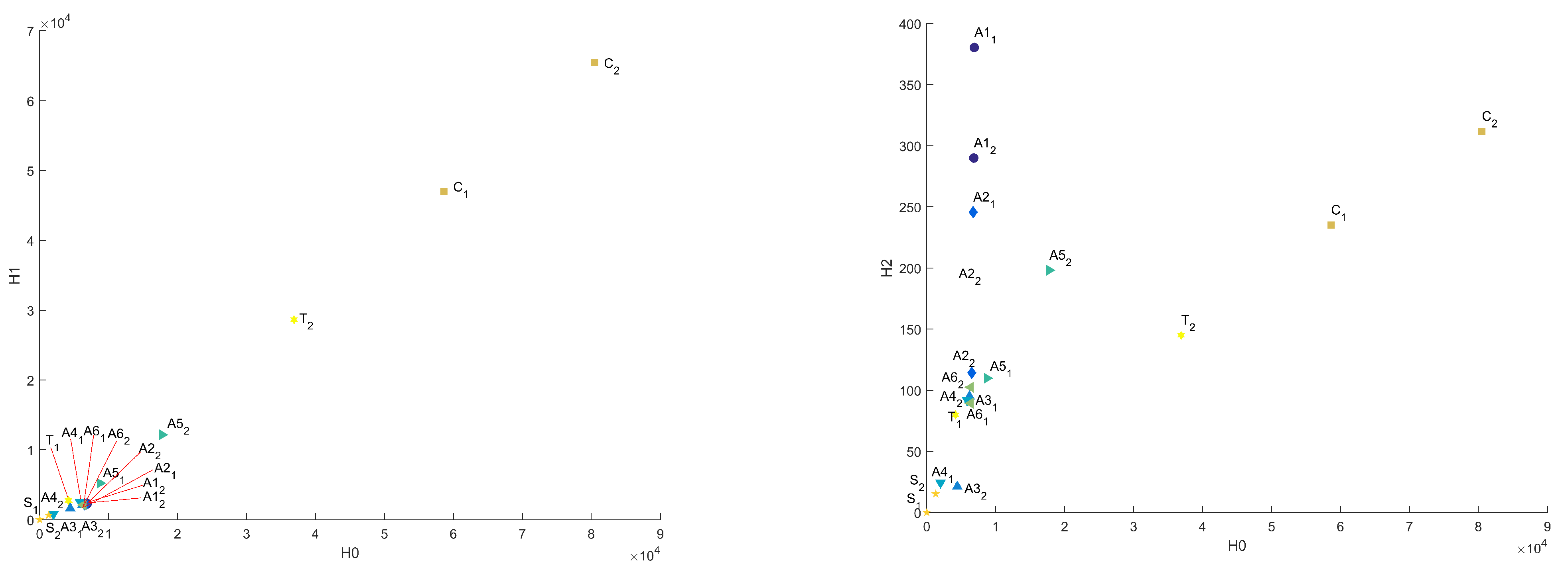
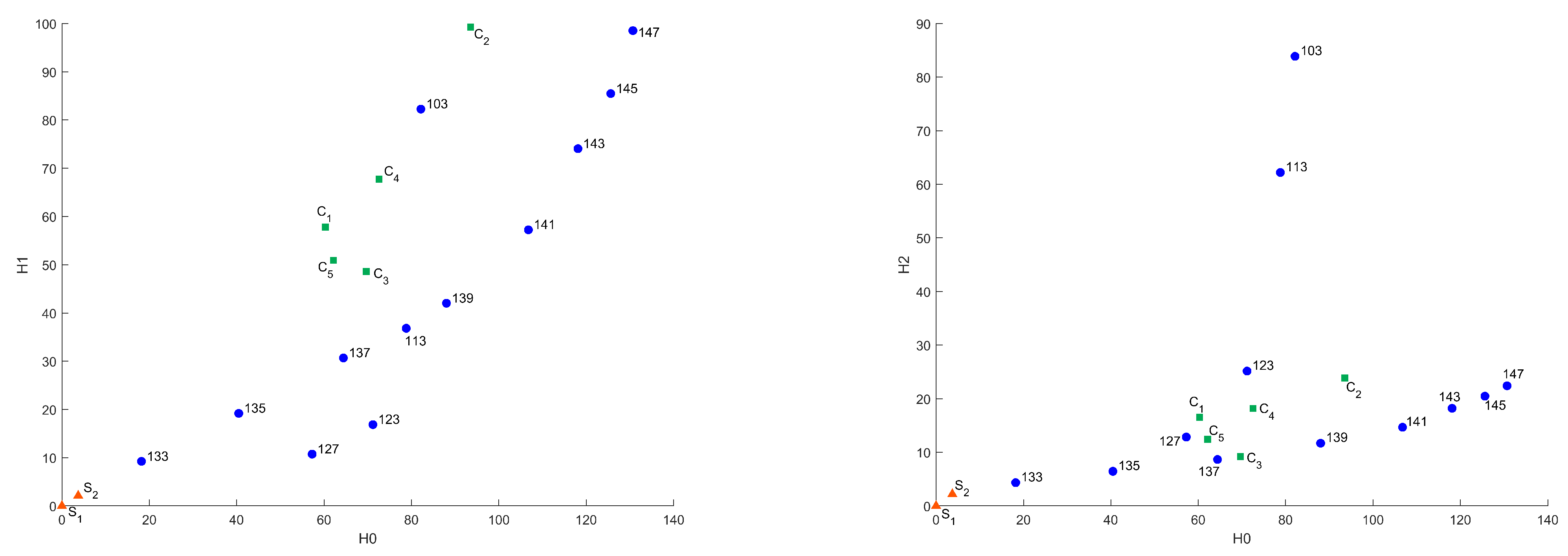
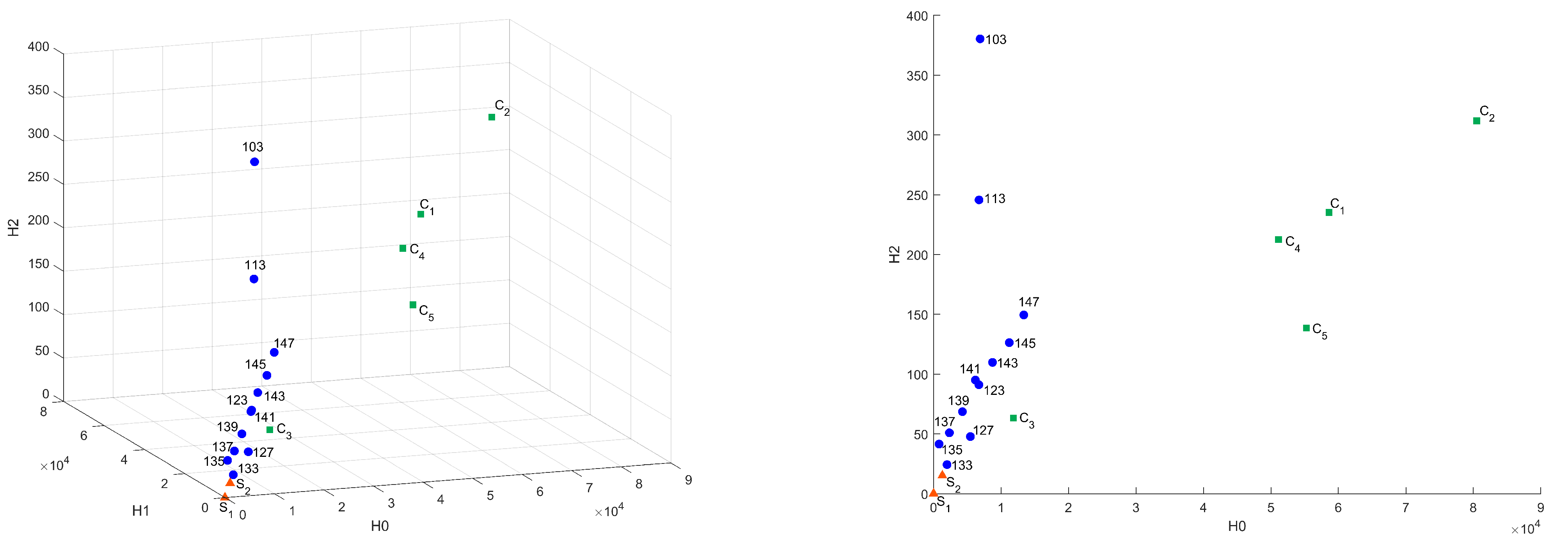
In Figure 9, Figure 10, Figure 11 and Figure 12, the influence of the binarization threshold of the A sample on the distance values from sample (“base” sample) in the Bottleneck, Heat Kernel, and Sliced Wasserstein metrics is shown (threshold value is marked as label for dots). In addition, five different subsamples of the C sample were taken for reference and marked as .
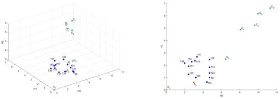
Figure 9.
Influence of the binarization threshold of A sample in Bottleneck metric in 3D and – coordinates.
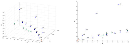
Figure 10.
Influence of the binarization threshold of A sample in Heat Kernel metric in 3D and – coordinates.
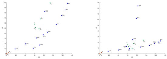
Figure 11.
Influence of the binarization threshold of A sample in Heat Kernel metric in – and – coordinates.
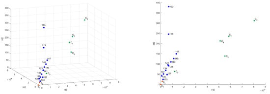
Figure 12.
Influence of the binarization threshold of A sample in Sliced Wasserstein metric in 3D and – coordinates.
It can be seen that changing the binarization threshold makes the A sample more similar to S sample in terms of surveyed metrics. It can be explained by eliminating tiny features and elements and by changing the considered scale. While transiting the inversion point of a binarized image, the differences start to arise—the details of microstructure appear. This effect is the same as while we change the resolution of the original CT image. This mechanism allows us to search for common on different scales or for different image quality. In this case, the C sample differs significantly from other samples on all considered scales because of fundamental differences in structure.
In Figure A3, CT slices with different binarization thresholds are presented.
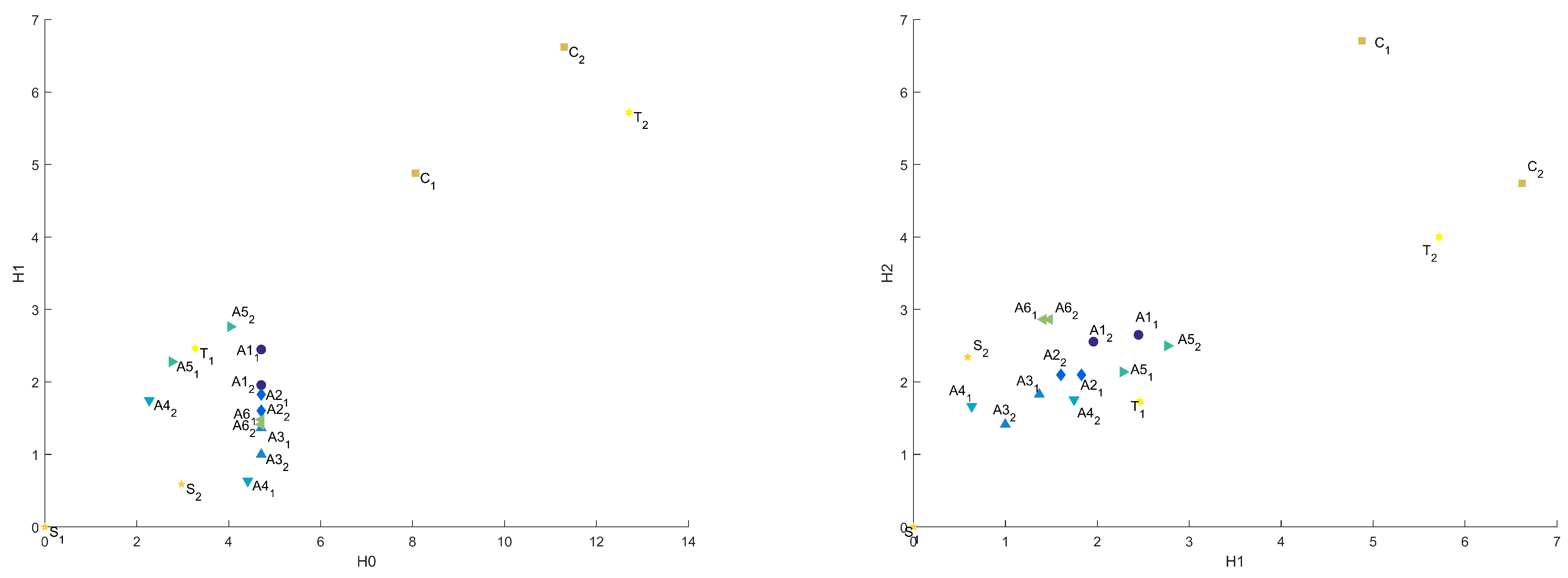
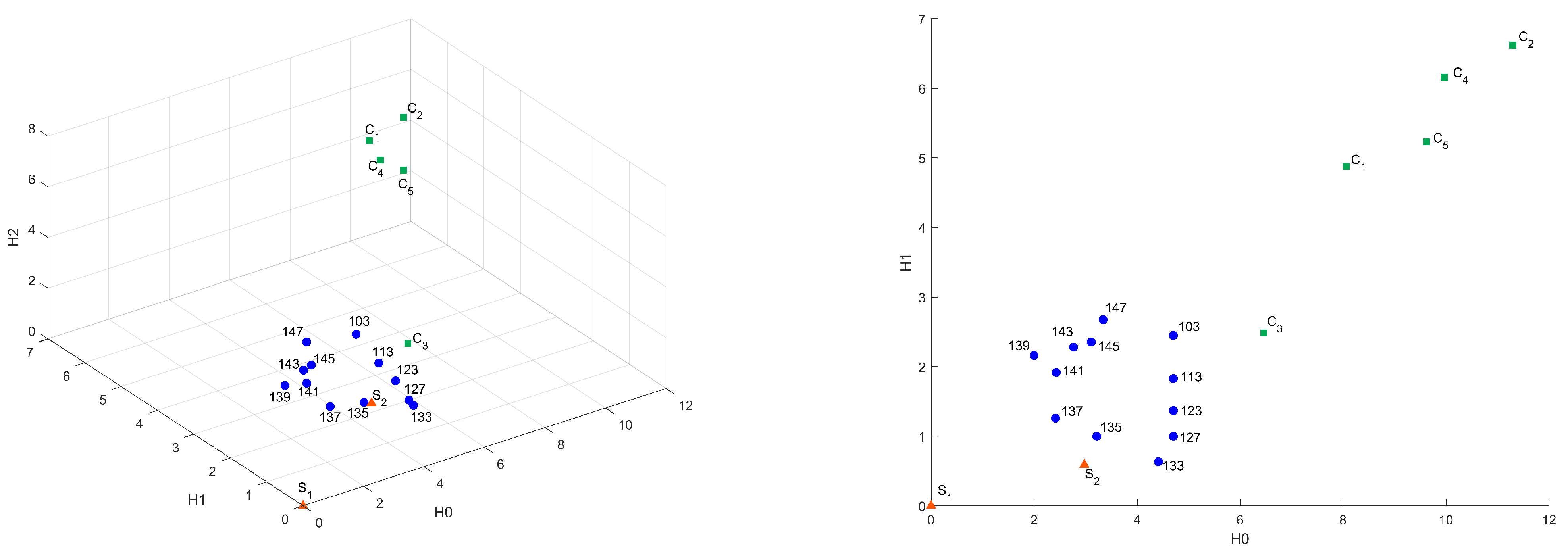
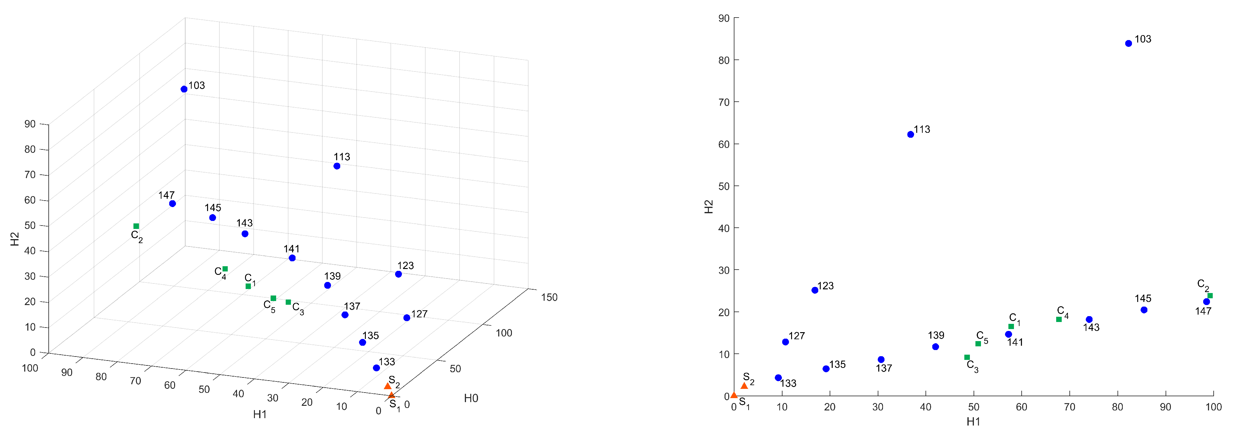
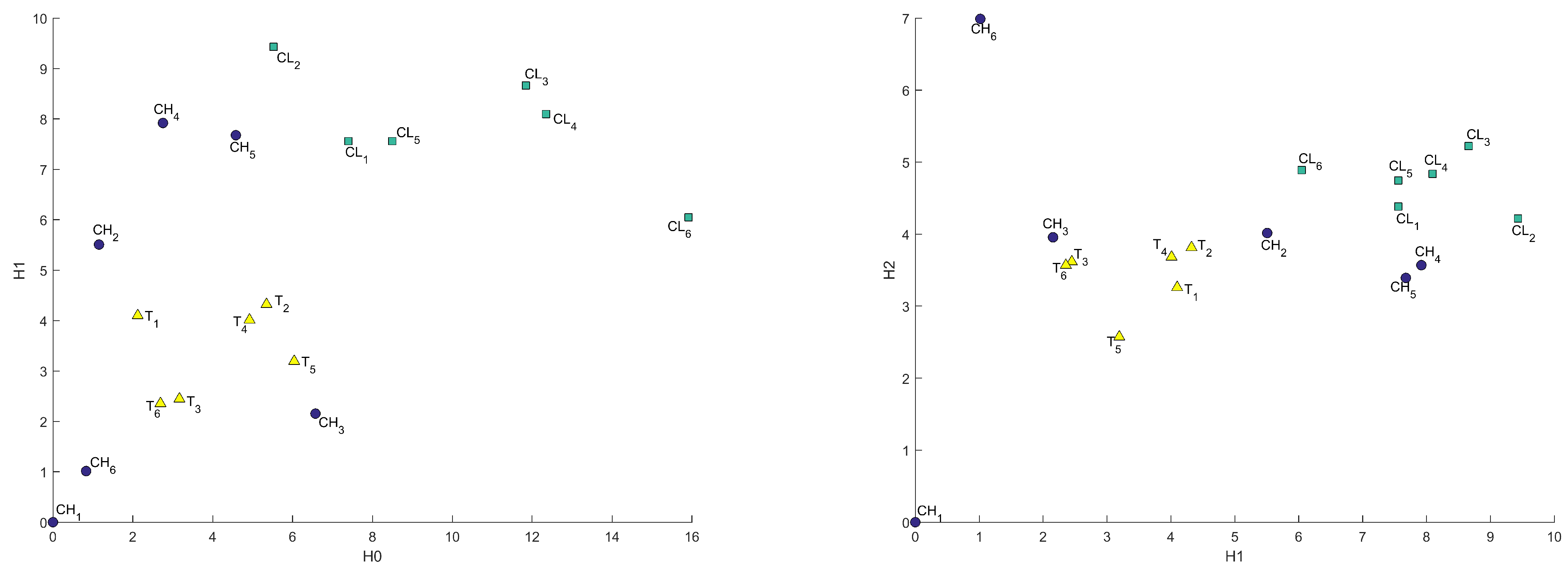
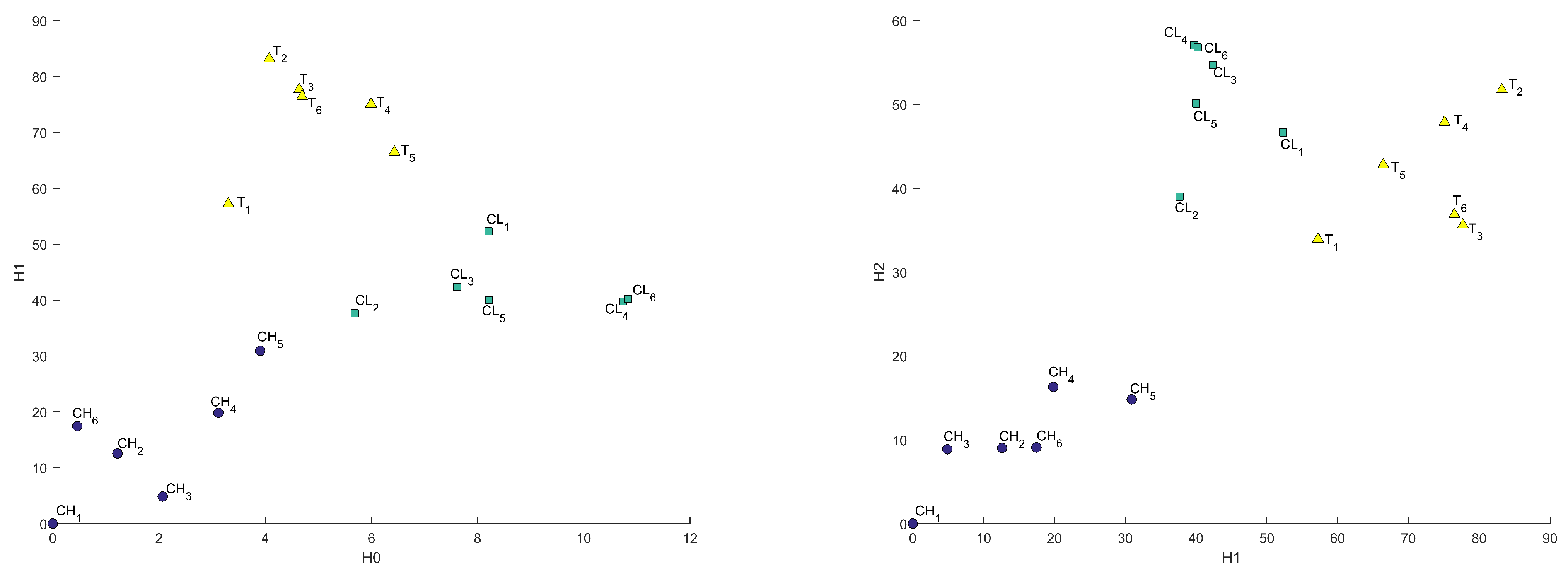
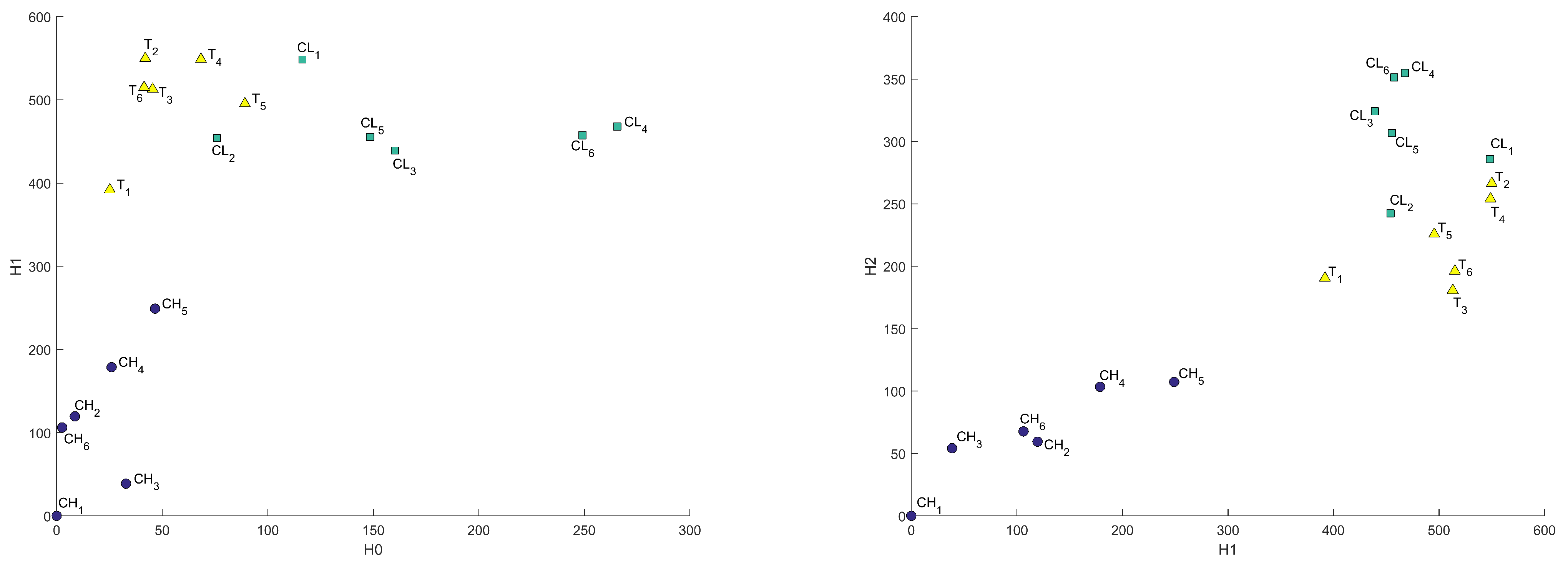
C sample was divided on two classes by porosity range and low-porosity samples were denoted as CL, high-porosity as CH, and B samples were taken for reference and were denoted as T. Results for these samples in all metrics are presented in Figure A2, Figure A3 and Figure 13, Figure 14 and Figure 15. As “base” sample was taken. We can see a good distinction between considered classes. It is worth noting that C sample groups with significantly different porosity have different genesis and evolution. However, there are still distinctions between low-porosity C and B samples, although they have similar porosity and permeability but different genesis.
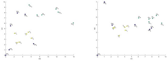
Figure 13.
Comparison of 2 classes of C (CH, CL) samples with T samples (T) in Bottleneck metric in – and – coordinates.
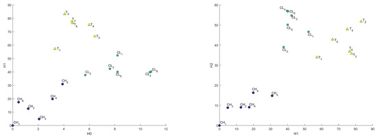
Figure 14.
Comparison of 2 classes of C (CH, CL) samples with T samples (T) in Heat Kernel metric in – and – coordinates.
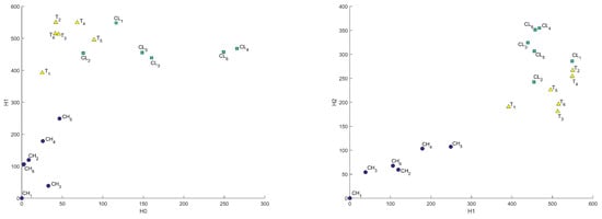
Figure 15.
Comparison of 2 classes of C (CH, CL) samples with T samples (T) in Sliced Wasserstein metric in – and – coordinates.
4. Discussion
The results show that the proposed algorithm is working well on studied samples: it classifies samples in all metrics and the most effective one is based on Heat Kernel. Calculation time is rather low: on average all the mentioned steps and calculations take less than an hour on a regular personal computer, which allows for quick calculations. Robustness and stability combined with a possibility to work in automated mode allow for a quick division of the samples into groups for further analysis or to find a sample that can be counted as a close structure analog to propose some a priori properties of the sample (if specific study procedure or sample preparation is needed). Compared to conventional methods, this approach can win when quick estimation is needed and time-consuming flow calculations are not suitable, or when classical statistical distribution classification is not working well. That case might happen when studied samples have complex or combined distributions or in the case of highly anisotropic samples. In that case, samples with quite formal distributions can have completely different properties due to the statistically rare microstructure objects that define integral sample properties. Taking into account topology allows using such objects for correct classification.
Another application is multiscale analysis, when samples have more than one distribution of microstructure objects such as pores or pore channels in one or different scales. In that case, it is quite hard to differentiate one from another just using statistics or cross-plots because distributions can interfere and peaks can be smoothed and hard to separate. As it happens, the proposed method also shows the possibility to separate distributions (as it was shown for subsamples of sample C) or even to separate scales with the use of threshold or resolution variations and make a multiscale classification in one automated calculation run. This might be useful to find dominating scale, find separate analogs for different scales of the same sample, or to check the possibility of some secondary formation processes that occurred with samples and thus generated some new distribution.
In addition, usage of the proposed method can somewhat elucidate the physical and chemical processes that happened during sample (porous media) formation and evolution because genesis processes are not completely random and microstructure is connected to the genesis process and thus that process can be partially reconstructed with the use of sample microstructure objects topology. This approach is widely used in lithology and facial geological analysis and the proposed method can be used as an instrument for such type of workflow. However, the exact correlation of topological properties with physical and chemical processes yet needs to be studied in further research with more samples with different genesis.
This methodology can be applied to many other complex structures with different scales. Due to the specifics and volume of the data we have accumulated in our work, we have chosen samples of hydrocarbon reservoirs for verification since they have been well studied using other methods, and many results have been accumulated on them.
Obtained results show four main methodology limitations:
- Calculation limitation: current maximum image size processed by the proposed workflow is 500 × 500 × 500, but it can be improved further by software and hardware optimization;
- High-quality images are required for adequate and precise calculations;
- Samples studied in this paper have quite different geometrical structures. More statistics are required to estimate the precision of the proposed method to separate samples with similar structure;
- The proposed algorithm takes into account only geometrical properties and yet ignores physical properties such as wettability/surface charge and so on.
The proposed algorithm was tested on a set of standard samples. In the future, it is planned to test the algorithm on a wider set of samples, which will allow a more detailed assessment of its advantages and limitations.
5. Conclusions
In this paper, a new method of 3D-structures classification is proposed, based on the topological data analysis methods, by constructing persistent diagrams of binarized images and qualitatively determining the similarity of samples in terms of the distances between persistent homologies in three different metrics.
- 1.
- The applicability of this method to the classification of hydrocarbon reservoir samples is shown. The procedure is described;
- 2.
- The algorithm is stable (linear response, small changes in input parameters lead to small changes in output) and could be highly automated;
- 3.
- The resolution and threshold of binarization affect the distance values (cluster size), but the clustering is preserved. It lasts as long as the objects are physically different: at certain thresholds, the samples become similar in visible structure, which means the cluster changes;
- 4.
- The proposed algorithm for classifying hydrocarbon reservoir samples makes it possible to classify the samples taking into account their microstructure and the topological properties of the porous media at different scales and to take into account genesis and the conditions for forming the sample which allows to study some physical/chemical/geological processes that occurred at that reservoir during formation stage. For example, Binarization or downscaling allows the search for commonalities in structure between different formations at different scales;
- 5.
- The most contrasting results of clustering of sample groups are obtained in the Heat Kernel metric.
Author Contributions
Conceptualization, E.G.; methodology, D.I. and A.F.; software, D.I. and A.F.; validation, P.G. and M.C.; formal analysis, E.G.; investigation, A.F.; resources, P.G.; data curation, P.G.; writing—original draft preparation, A.F.; writing—review and editing, A.F., P.G., and D.I.; visualization, A.F.; supervision, E.G.; project administration, E.G.; funding acquisition, P.G. All authors have read and agreed to the published version of the manuscript.
Funding
This work was supported by the Ministry of Science and Higher Education of the Russian Federation under agreement No. 075-10-2020-119 within the framework of the development program for a world-class Research Center.
Institutional Review Board Statement
Not applicable.
Informed Consent Statement
Not applicable.
Data Availability Statement
Not applicable.
Acknowledgments
The authors thank the two anonymous referees for taking the time to review our manuscript and for their helpful comments, which have improved the manuscript.
Conflicts of Interest
The authors declare no conflict of interest.
Appendix A. 3D Graphics
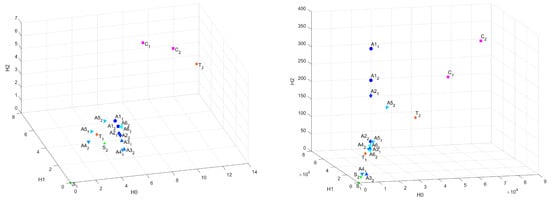
Figure A1.
3D-plot of common distances in Bottleneck and Sliced Wasserstein metrics.
Figure A1.
3D-plot of common distances in Bottleneck and Sliced Wasserstein metrics.
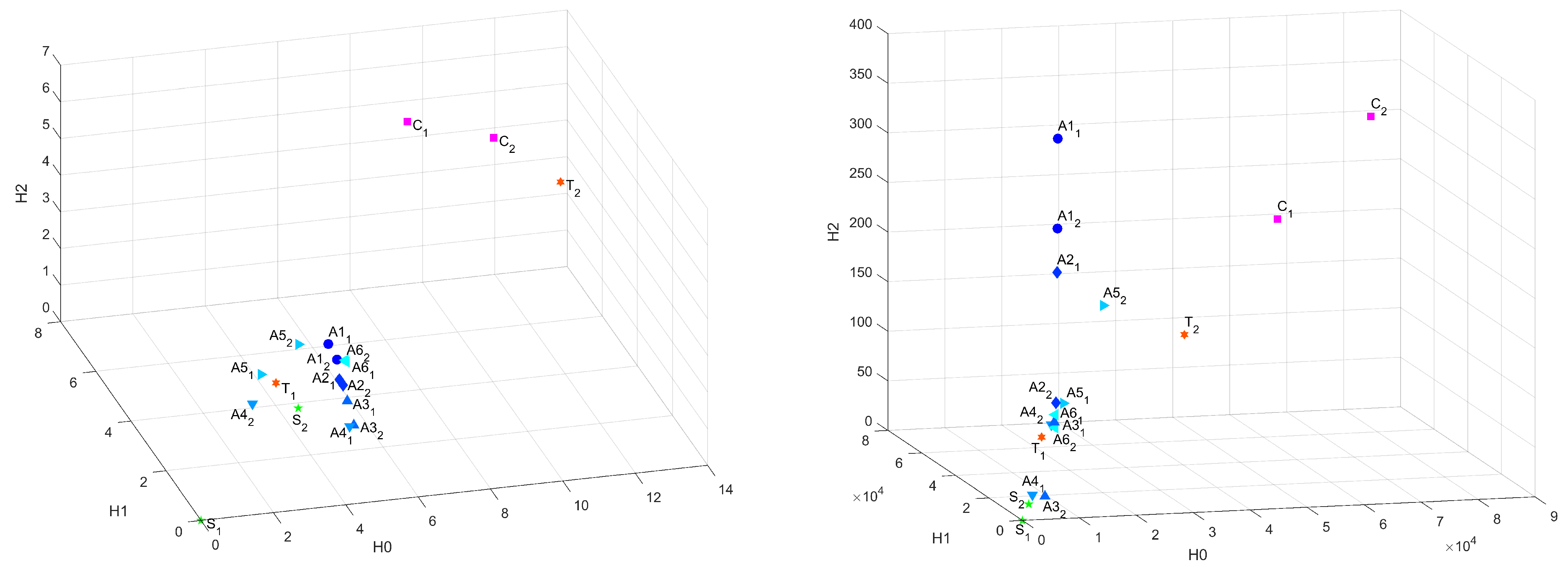
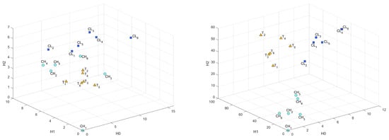
Figure A2.
Comparison of 2 classes of C (CH, CL) samples with T samples (T) in Bottleneck and Heat Kernel metrics in 3D coordinates.
Figure A2.
Comparison of 2 classes of C (CH, CL) samples with T samples (T) in Bottleneck and Heat Kernel metrics in 3D coordinates.
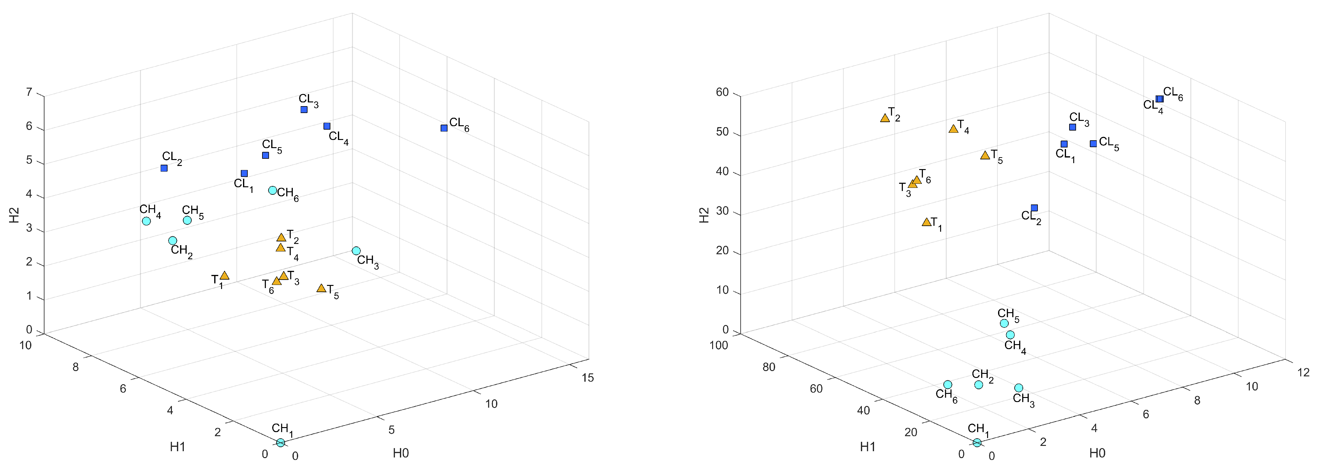

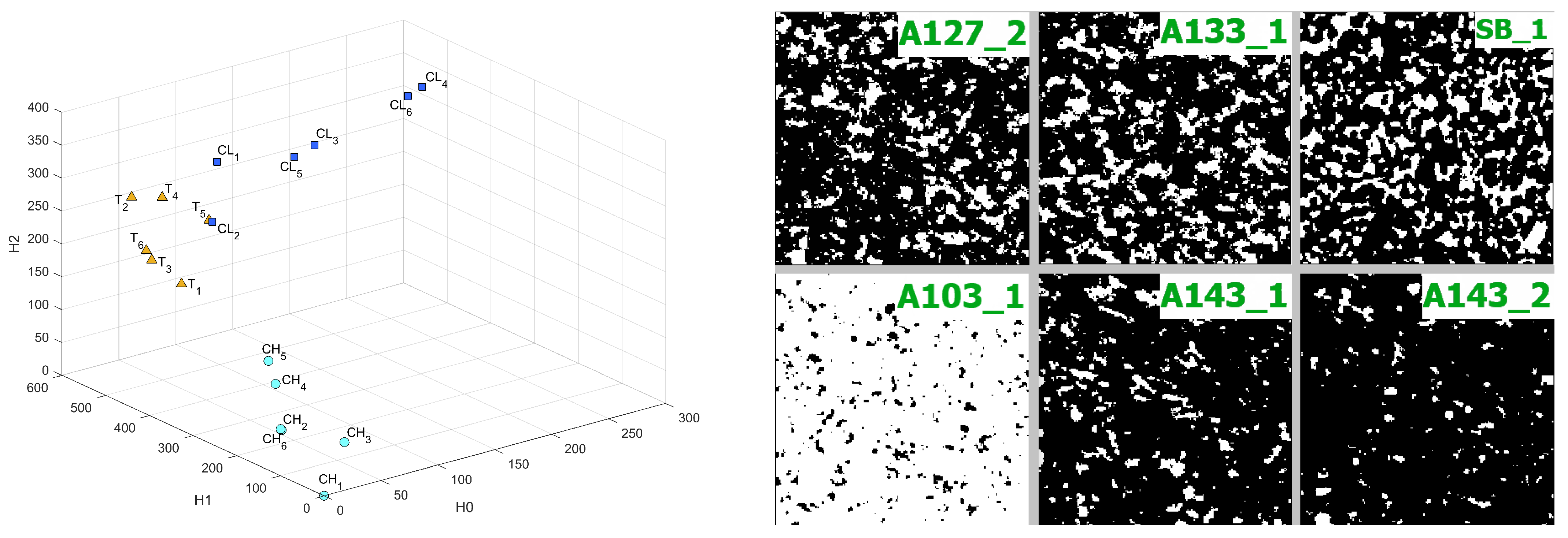
Figure A3.
Comparison of 2 classes of C (CH, CL) samples with T samples (T) in Sliced Wasserstein metric in 3D coordinates (left figure) and example of sample’s slices with different binarization threshold. A denotes A sample, SB—Sandstone, numbers denote threshold, underscore denotes the number of subsample (right figure).
References
- Hounsfield, G.N. A Method of and Apparatus for Examination of a Body by Radiation Such as X-or Gamma-radiation. British Patent No. 1,283,915, 1972. [Google Scholar]
- Hounsfield, G.N. Computerized transverse axial scanning (tomography): Part 1. Description of system. Br. J. Radiol. 1973, 46, 1016–1022. [Google Scholar] [CrossRef]
- Petrovic, A.; Siebert, J.; Rieke, P. Soil bulk density analysis in three dimensions by computed tomographic scanning. Soil Sci. Soc. Am. J. 1982, 46, 445–450. [Google Scholar] [CrossRef]
- Hainsworth, J.; Aylmore, L. The use of computer assisted tomography to determine spatial distribution of soil water content. Soil Res. 1983, 21, 435–443. [Google Scholar] [CrossRef]
- Arnold, J.; Testa, J.; Friedman, P.; Kambic, G. Computed tomographic analysis of meteorite inclusions. Science 1983, 219, 383–384. [Google Scholar] [CrossRef] [Green Version]
- Haubitz, B.; Prokop, M.; Dohring, W.; Ostrom, J.; Wellnhofer, P. Computed tomography of Archaeopteryx. Paleobiology 1988, 14, 206–213. [Google Scholar] [CrossRef]
- Raynaud, S.; Fabre, D.; Mazerolle, F.; Geraud, Y.; Latière, H.J. Analysis of the internal structure of rocks and characterization of mechanical deformation by a non-destructive method: X-ray tomodensitometry. Tectonophysics 1989, 159, 149–159. [Google Scholar] [CrossRef]
- Renter, J.A. Applications of computerized tomography in sedimentology. Mar. Georesources Geotechnol. 1989, 8, 201–211. [Google Scholar] [CrossRef]
- Karsanina, M.V.; Lavrukhin, E.V.; Fomin, D.S.; Yudina, A.V.; Abrosimov, K.N.; Gerke, K.M. Compressing soil structural information into parameterized correlation functions. Eur. J. Soil Sci. 2021, 72, 561–577. [Google Scholar] [CrossRef]
- Serra, J. Image analysis and mathematical morphology. IEEE Trans. Pattern Anal. Mach. Intell. 1982, 4, 532–550. [Google Scholar]
- Gong, L.; Nie, L.; Xu, Y. Geometrical and topological analysis of pore space in sandstones based on x-ray computed tomography. Energies 2020, 13, 3774. [Google Scholar] [CrossRef]
- Ivonin, D.; Grishin, P.; Grachev, E. Quantitative Analysis of Samples of Natural Hydrocarbon Reservoirs by the Methods of Integral Geometry and Topology. Izv. Phys. Solid Earth 2021, 57, 366–374. [Google Scholar] [CrossRef]
- Vogel, H.J.; Weller, U.; Schlüter, S. Quantification of soil structure based on Minkowski functions. Comput. Geosci. 2010, 36, 1236–1245. [Google Scholar] [CrossRef]
- Lucas, M.; Vetterlein, D.; Vogel, H.J.; Schlüter, S. Revealing pore connectivity across scales and resolutions with X-ray CT. Eur. J. Soil Sci. 2021, 72, 546–560. [Google Scholar] [CrossRef] [Green Version]
- Muñoz Ortega, F.J. Geometrical Characterization of Undisturbed Soil Samples Using X-ray Computed Tomography Image Analysis. Effect of Soil Management on Soil Structure. Ph.D. Thesis, The Technical University of Madrid (UPM), Madrid, Spain, 2015. [Google Scholar]
- Pabst, W.; Uhlířová, T.; Gregorová, E. Microstructure characterization of porous ceramics via Minkowski functionals. In Ceramic Transactions Series; Singh, D., Fukushima, M., Kim, Y.-W., Shimamura, K., Imanaka, N., Ohji, T., Amoroso, J., Lanagan, M., Eds.; John Wiley & Sons, Inc.: Hoboken, NJ, USA, 2018; pp. 53–64. ISBN 978-1-119-49409-6. [Google Scholar]
- Gregorová, E.; Uhlířová, T.; Pabst, W.; Diblíková, P.; Sedlářová, I. Microstructure characterization of mullite foam by image analysis, mercury porosimetry and X-ray computed microtomography. Ceram. Int. 2018, 44, 12315–12328. [Google Scholar] [CrossRef]
- Kader, M.; Brown, A.; Hazell, P.; Robins, V.; Escobedo, J.; Saadatfar, M. Geometrical and topological evolution of a closed-cell aluminium foam subject to drop-weight impact: An X-ray tomography study. Int. J. Impact Eng. 2020, 139, 103510. [Google Scholar] [CrossRef]
- Tsukanov, A.; Ivonin, D.; Gotman, I.; Gutmanas, E.Y.; Grachev, E.; Pervikov, A.; Lerner, M. Effect of Cold-Sintering Parameters on Structure, Density, and Topology of Fe–Cu Nanocomposites. Materials 2020, 13, 541. [Google Scholar] [CrossRef] [Green Version]
- Gilmanov, R.R.; Kalyuzhnyuk, A.V.; Taimanov, I.A.; Yakovlev, A.A. Topological characteristics of digital models of geological core. In International Cross-Domain Conference for Machine Learning and Knowledge Extraction; Springer: Berlin/Heidelberg, Germany, 2018; pp. 273–281. [Google Scholar]
- Ivonin, D.; Kalnin, T.; Grachev, E.; Shein, E. Quantitative Analysis of Pore Space Structure in Dry and Wet Soil by Integral Geometry Methods. Geosciences 2020, 10, 365. [Google Scholar] [CrossRef]
- Robins, V. Towards computing homology from finite approximations. Topol. Proc. 1999, 24, 503–532. [Google Scholar]
- Edelsbrunner, H.; Harer, J. Persistent homology—A survey. Contemp. Math. 2008, 453, 257–282. [Google Scholar]
- Letscher, H.; Zomorodian, A. Topological persistence and simplification. Discret. Comput. Geom. 2002, 28, 511–533. [Google Scholar]
- Cohen-Steiner, D.; Edelsbrunner, H.; Harer, J. Stability of persistence diagrams. Discret. Comput. Geom. 2007, 37, 103–120. [Google Scholar] [CrossRef] [Green Version]
- Murakami, M.; Kohara, S.; Kitamura, N.; Akola, J.; Inoue, H.; Hirata, A.; Hiraoka, Y.; Onodera, Y.; Obayashi, I.; Kalikka, J.; et al. Ultrahigh-pressure form of Si O 2 glass with dense pyrite-type crystalline homology. Phys. Rev. B 2019, 99, 045153. [Google Scholar] [CrossRef] [Green Version]
- Moon, C.; Li, Q.; Xiao, G. Predicting survival outcomes using topological features of tumor pathology images. arXiv 2020, arXiv:2012.12102. [Google Scholar]
- Oyama, A.; Hiraoka, Y.; Obayashi, I.; Saikawa, Y.; Furui, S.; Shiraishi, K.; Kumagai, S.; Hayashi, T.; Kotoku, J. Hepatic tumor classification using texture and topology analysis of non-contrast-enhanced three-dimensional T1-weighted MR images with a radiomics approach. Sci. Rep. 2019, 9, 1–10. [Google Scholar] [CrossRef]
- Armstrong, R.T.; McClure, J.E.; Robins, V.; Liu, Z.; Arns, C.H.; Schlüter, S.; Berg, S. Porous media characterization using Minkowski functionals: Theories, applications and future directions. Transp. Porous Media 2019, 130, 305–335. [Google Scholar] [CrossRef]
- Hiraoka, Y.; Nakamura, T.; Hirata, A.; Escolar, E.G.; Matsue, K.; Nishiura, Y. Hierarchical structures of amorphous solids characterized by persistent homology. Proc. Natl. Acad. Sci. USA 2016, 113, 7035–7040. [Google Scholar] [CrossRef] [Green Version]
- Saadatfar, M.; Takeuchi, H.; Robins, V.; Francois, N.; Hiraoka, Y. Pore configuration landscape of granular crystallization. Nat. Commun. 2017, 8, 1–11. [Google Scholar] [CrossRef]
- Robins, V.; Turner, K. Principal component analysis of persistent homology rank functions with case studies of spatial point patterns, sphere packing and colloids. Phys. D Nonlinear Phenom. 2016, 334, 99–117. [Google Scholar] [CrossRef] [Green Version]
- Robins, V.; Saadatfar, M.; Delgado-Friedrichs, O.; Sheppard, A.P. Percolating length scales from topological persistence analysis of micro-CT images of porous materials. Water Resour. Res. 2016, 52, 315–329. [Google Scholar] [CrossRef] [Green Version]
- Suzuki, A.; Miyazawa, M.; Minto, J.M.; Tsuji, T.; Obayashi, I.; Hiraoka, Y.; Ito, T. Flow estimation solely from image data through persistent homology analysis. Sci. Rep. 2021, 11, 1–13. [Google Scholar] [CrossRef]
- Jiang, F.; Tsuji, T.; Shirai, T. Pore geometry characterization by persistent homology theory. Water Resour. Res. 2018, 54, 4150–4163. [Google Scholar] [CrossRef]
- Delgado-Friedrichs, O.; Robins, V.; Sheppard, A. Morse theory and persistent homology for topological analysis of 3d images of complex materials. In Proceedings of the 2014 IEEE International Conference on Image Processing (ICIP), Paris, France, 27–30 October 2014; pp. 4872–4876. [Google Scholar]
- Moon, C.; Mitchell, S.A.; Heath, J.E.; Andrew, M. Statistical inference over persistent homology predicts fluid flow in porous media. Water Resour. Res. 2019, 55, 9592–9603. [Google Scholar] [CrossRef]
- Arns, J.Y.; Robins, V.; Sheppard, A.P.; Sok, R.M.; Pinczewski, W.V.; Knackstedt, M.A. Effect of network topology on relative permeability. Transp. Porous Media 2004, 55, 21–46. [Google Scholar] [CrossRef]
- Herring, A.; Robins, V.; Sheppard, A. Topological persistence for relating microstructure and capillary fluid trapping in sandstones. Water Resour. Res. 2019, 55, 555–573. [Google Scholar] [CrossRef] [Green Version]
- Tsuji, T.; Jiang, F.; Suzuki, A.; Shirai, T. Mathematical modeling of rock pore geometry and mineralization: Applications of persistent homology and random walk. In Forum “Math-for-Industry”; Springer: Berlin/Heidelberg, Germany, 2016; pp. 95–109. [Google Scholar]
- Khachkova, T.S.; Bazaikin, Y.V.; Lisitsa, V.V. Use of the computational topology to analyze the pore space changes during chemical dissolution. Numer. Methods Progr. 2020, 21, 41–55. [Google Scholar]
- Prokhorov, D.I.; Bazaikin, Y.V.; Lisitsa, V.V. Digital image reduction for analysis of topological changes in the pore space of the rock matrix during chemical dissolution. Numer. Methods Progr. 2020, 21, 319–328. [Google Scholar]
- Ichinomiya, T.; Obayashi, I.; Hiraoka, Y. Persistent homology analysis of craze formation. Phys. Rev. E 2017, 95, 012504. [Google Scholar] [CrossRef] [Green Version]
- Kimura, M.; Obayashi, I.; Takeichi, Y.; Murao, R.; Hiraoka, Y. Non-empirical identification of trigger sites in heterogeneous processes using persistent homology. Sci. Rep. 2018, 8, 1–9. [Google Scholar] [CrossRef] [Green Version]
- Buchet, M.; Hiraoka, Y.; Obayashi, I. Persistent homology and materials informatics. In Nanoinformatics; Springer: Singapore, 2018; pp. 75–95. [Google Scholar]
- Obayashi, I.; Hiraoka, Y.; Kimura, M. Persistence diagrams with linear machine learning models. J. Appl. Comput. Topol. 2018, 1, 421–449. [Google Scholar] [CrossRef] [Green Version]
- Ye, Q.Z. Signed Euclidean Distance Transform Applied to Shape Analysis. In Issues on Machine Vision; Springer: Berlin/Heidelberg, Germany, 1989; pp. 249–262. [Google Scholar]
- Delgado-Friedrichs, O.; Robins, V.; Sheppard, A. Skeletonization and partitioning of digital images using discrete morse theory. IEEE Trans. Pattern Anal. Mach. Intell. 2014, 37, 654–666. [Google Scholar] [CrossRef] [PubMed]
- Robins, V.; Wood, P.J.; Sheppard, A.P. Theory and algorithms for constructing discrete Morse complexes from grayscale digital images. IEEE Trans. Pattern Anal. Mach. Intell. 2011, 33, 1646–1658. [Google Scholar] [CrossRef] [PubMed]
- Peksa, A.E.; Wolf, K.H.A.; Slob, E.C.; Chmura, Ł.; Zitha, P.L. Original and pyrometamorphical altered Bentheimer sandstone; petrophysical properties, surface and dielectric behavior. J. Pet. Sci. Eng. 2017, 149, 270–280. [Google Scholar] [CrossRef] [Green Version]
- Peksa, A.E.; Wolf, K.H.A.; Zitha, P.L. Bentheimer sandstone revisited for experimental purposes. Mar. Pet. Geol. 2015, 67, 701–719. [Google Scholar] [CrossRef]
- Sheppard, A.; Sok, R.; Averdunk, H. Improved pore network extraction methods. Int. Symp. Soc. Core Anal. 2005, 2125, 1–11. [Google Scholar]
- Han, S.M.; Okonek, T.; Yadav, N.; Zheng, X. Distributions of Matching Distances in Topological Data Analysis. arXiv 2018, arXiv:1812.11258. [Google Scholar]
- Villani, C. Optimal Transport: Old and New; Springer: Berlin/Heidelberg, Germany, 2009; Volume 338. [Google Scholar]
- Carriere, M.; Cuturi, M.; Oudot, S. Sliced wasserstein kernel for persistence diagrams. In Proceedings of the International Conference on Machine Learning, Sydney, NSW, Australia, 6–11 August 2017; pp. 664–673. [Google Scholar]
- Santambrogio, F. Optimal transport for applied mathematicians. Birkäuser NY 2015, 55, 94. [Google Scholar]
- Reininghaus, J.; Huber, S.; Bauer, U.; Kwitt, R. A stable multi-scale kernel for topological machine learning. In Proceedings of the IEEE Conference on Computer Vision and Pattern Recognition, Boston, MA, USA, 7–12 June 2015; pp. 4741–4748. [Google Scholar]
Publisher’s Note: MDPI stays neutral with regard to jurisdictional claims in published maps and institutional affiliations. |
© 2021 by the authors. Licensee MDPI, Basel, Switzerland. This article is an open access article distributed under the terms and conditions of the Creative Commons Attribution (CC BY) license (https://creativecommons.org/licenses/by/4.0/).