Parameter Observer Useable for the Condition Monitoring of a Capacitor

Abstract

Monitoring the condition of electrolytic capacitors in practical applications is a topic that has been and remains the subject of much research. This article is part of research in this area. It develops a parameter observer (PO) and proposes its use for the determination of the equivalent capacity and equivalent serial resistance of electrolytic capacitors. The observer is an integral-open-loop type second-order system, the input of which is the voltage at the capacitor terminals measured during a two-stage capacitor’s discharging process through a variable resistor. The PO estimates the so-called time constant of the discharging circuit for each of the two stages from which values the capacitor’s parameters are calculated. The use of PO is illustrated for determining the output capacitor parameters of a buck DC–DC converter. The experiments were performed with two electrolytic capacitors with the nominal values 100 μF and 470 μF. Compared with other monitoring methods that use observers, the proposed observer is faster in tracking error mitigation, e.g., 10⁻³ s in comparison with 5·10⁻³ s or more. The low computational volume of the discrete-time PO allows the prospect of implementation in real time.

1. Introduction

Electrolytic capacitors are characterized by high electrical capacity/volume ratio, low internal resistance, and last but not least, their low price. These features are of great importance for various applications in the field of short-term electricity storage [1]. However, capacitors are vulnerable devices, responsible for numerous failures [2,3,4]. The high frequency of failures caused by electrolytic capacitors imposes the requirement of monitoring their equivalent parameters, mainly the capacitance (C) decreasing and the equivalent serial resistance (ESR) increasing, as part of condition monitoring. Much electronic equipment in the aerospace, medical, military or energy domains requires high reliability [5], and, consequently, fault diagnosis or maintenance based on monitoring the ESR and the capacitance of electrolytic capacitors [6,7,8] to ensure that they operate within the required degradation model [9].

There are more recent studies on the operational safety of equipment, in particular of power converters, from several perspectives. A wide range of analysis and decision-making techniques are used for this purpose, nowadays reaching the use of machine learning techniques [10,11,12]. Specific interfaces and algorithms, suitable for interaction with converters, are required for their application. Article [13] considers an ESR monitoring scheme without a current sensor, based on the calculation of the parameter’s values from the measurement of the AC component of the output voltage at precise times of the output switching cycle. In [14] a method of ESR monitoring is proposed based on the jump of the output voltage and the measurement of the ripple voltage output and inductor current. A model-free predictive control strategy, for the online estimation of the ESR and capacitance, aimed at the continuous evaluation of the electrolytic capacitor condition is discussed in [4]. The capacitor current and output voltage acquisitions are required.

The design of electronic circuits involving electrolytic capacitors uses different conceptual electrical models of capacitors, more or less simplified, and equivalent electrical parameters [5,15,16]. Simple models, type R-C, are widely used in modelling the circuits in which the capacitors are embedded, particularly in DC–DC converters [17]. In practice, C and ESR, the main parameters of electrolytic capacitors, vary substantially depending on the operating mode (voltage waveform, working frequency and temperature), but also due to the irreversible aging phenomenon [18]. During the transient phenomena, characteristic of electric charging–discharging cycles, there is a reversible variation in the values of the main parameters of the electrolytic capacitors. In [19] this behaviour is highlighted for a capacitor discharging process.

A comprehensive and topical synthesis regarding monitoring dc-link capacitors in power converters is presented in [7]. It highlights the equivalent conceptual schemes and estimation principles used. From the perspective of our research, we note the equivalent scheme R-C, used when the equivalent series inductance is negligible, as well as the principle of the model-based estimation in the non-periodic discharging profile variant. It is also worth noting the study in [20], which addresses the monitoring of the output capacitor and the inductor of a boost converter, considering for the capacitor an equivalent R-C model.

The authors of [8] propose a method of online monitoring of the ESR and C of the output capacitor of a buck converter based on the analysis of the transient voltage regimes at the terminals of the output capacitor. In the same vein, [6] presents a condition-monitoring procedure for dc-link capacitors of AC–DC–AC power converters based on a variable electrical network capable of estimating the equivalent C and the equivalent ESR of the dc-link capacitor. No current sensor was used in either study, and no external signal was injected.

Observers are widely used in technology as tools for extracting information from a dynamic system. They are continuous-time or discrete-time dynamic systems, which contain, as appropriate, models of the observed system and/or models of external signals incident to the observed system. The observers approximate, depending on the situation, the signals from the observed system or incident signals, or combinations thereof [21,22]. Generally, in a technical solution, observers are implemented as a software function of the electronic control unit, contributing to various operations such as measurement, protection, condition monitoring, etc. A unified characterization of the state and disturbance observers can be found in [23]. The area of use of the observers mainly includes control and measurement applications in many fields, including DC–DC converters, e.g., [24], but also fault diagnosis via observer-based detection filters [25], or attack detection on sensor areas in cyber–physical systems [26]. Cen and Stewart in [3], Jain et al. in [27] and Meng et al. in [28] adopt a different approach, which falls into the category of estimating the parameters of electrical circuits. In [3], three continuous-time observers are used, one for the fault diagnosis of a buck converter and two, depending on the fault’s localization, for the inductance estimation of the converter and for the capacitance estimation of the output capacitor of the converter. Ref. [27] develops an improved robust adaptive parameter identifier for DC–DC power electronic converters that use a continuous-time observer with amplifications designed using the H∞-type performance criterion. The use is aimed at both the capacitor and inductance of the output stage of a DC–DC boost converter. Paper [28] proposes for the output capacitor of a boost converter two parameter observers, one for ESR and one for C. Both use the R-C model of the capacitor in structures that have as inputs, in addition to the capacitor’s voltage, at least one more current signal. A 100 Hz signal is injected to trigger the estimation process in the diagram.

In this paper, we present a new type of observer, called parameter observer (PO), designed for first-order systems, in a free regime. The new idea is to transform the parameter into a state variable. We associate the main purpose with the illustration of the possibility of using the PO to calculate the values of the equivalent parameters of the final filter electrolytic capacitor of a DC–DC buck source. The PO monitors the so-called time constant of the capacitor discharging circuit through a resistor using only the voltage at the capacitor terminals. The method for determining the equivalent parameters of the capacitor is by dividing the discharging process of the capacitor into two stages. In [6] the dividing is carried out in three stages. From the viewpoint of the structure, the proposed observer falls into the category of open-loop observers [29], and from the viewpoint of treating the observation errors in the category of proportional integral observers [23].

Section 2 of the article describes the operating principle of the proposed parameter observer in both the continuous-time version and the discrete-time version, respectively, the method by which the equivalent parameters of an electrolytic capacitor are determined with its help. The results calculated with the PO from offline-processed experimental data are shown in Section 3. The discussion in Section 4 is intended to assess the applicability of the parameter observer. The last section summarizes the contributions of this paper.

All experimental data processing and simulations were performed using the MATLAB-SIMULINK environment.

2. Materials and Methods

This section presents the concept of a parametric observer usable for determining the time constant of a first-order continuous-time linear system from the free response of the system and a method of its use for determining the equivalent values of ESR and the capacitance of an electrolytic capacitor.

The parameter observer is presented in both the continuous-time and the discrete-time version.

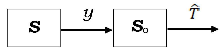
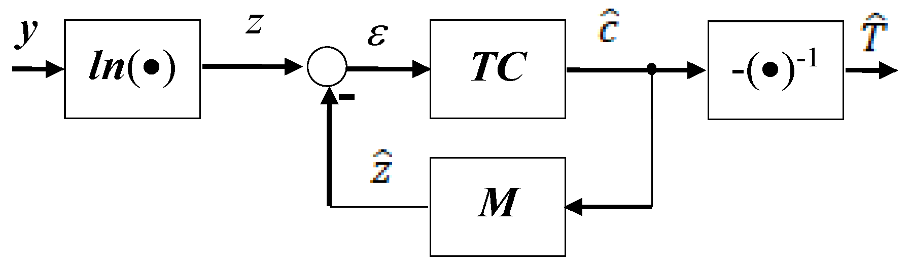
2.1. Continuous-Time Observer for Determining the Variation of the Parameters of a First-Order Continuous-Time System from Its Non-Sampled Free Response

In Figure 1, the block S is the first-order system (1) and S₀ is an observer of the parameter T, hereinafter, parameter observer (PO). The function of PO is to indirectly measure the value of T during the free regime of the system S:

$$T\left(t\right)\dot{y}\left(t\right)+y\left(t\right)=0, y\left(0\right)=y_0.$$

(1)

We assume that throughout the free regime determined by the initial state y₀ are met the conditions: y is measurable, $\dot{y}\left(t\right)\ne 0$, and T(t)$>0$.

The operating principle of S₀ is suggested by rewriting the model (1) in form (2):

$$T\left(t\right)\dot{z}\left(t\right)+1=0 ,z\left(0\right)=z_0=\ln \left(y_0\right),$$

(2)

where

$$z\left(t\right)=ln\left(y\left(t\right)\right).$$

(3)

Since $T\left(t\right)>0,$we define the variable:

$$c\left(t\right)=-\frac{1}{T\left(t\right)} ,$$

(4)

and model (2) becomes

$$\dot{z}\left(t\right)=c\left(t\right), z\left(0\right)=z_0.$$

(5)

As a result of the above substitutions, the problem of estimating T(t) becomes the problem of tracking the variable c(t) with an observer S₀ that includes the model (5). The structure in Figure 2, in which M is the model (5) rewritten as (6), and TC is a tracking controller of z(t), can perform the tracking of T(t). The input block performs the operation (3), and the output block performs the operation (7), opposite to the one in (4):

$$d\widehat{z}/dt=\widehat{c}\left(t\right), \widehat{z}\left(0\right)={\widehat{z}}_0,$$

(6)

$$\widehat{T}\left(t\right)=-\frac{1}{\widehat{c}\left(t\right)} .$$

(7)

The tracking error,

$$\epsilon \left(t\right)=z\left(t\right)-\widehat{z}\left(t\right),$$

(8)

must approach asymptotically to 0, and for this reason, the controller should have an integrative character. We adopt the structure (9) of the PI type:

$$\widehat{c}\left(t\right)=K_p\epsilon \left(t\right)+K_i{\int }_0^t\epsilon \left(\tau \right)d\tau +{\widehat{c}}_0,$$

(9)

where ${\widehat{c}}_0$ is the initial value of $\widehat{c}\left(t\right)$.

Equations (6), (8) and (9) together represent the mathematical model of the tracking subsystem. It provides the linking Equation (10) between the Laplace images of the input signal to the subsystem and the initial conditions, on the one hand, and the tracking error, on the other hand:

$$\epsilon \left(s\right)=\frac{s^2}{s^2+K_p·s+K_i}·z\left(s\right)-\frac{s}{s^2+K_p·s+K_i}·{\widehat{z}}_0-\frac{1}{s^2+K_p·s+K_i}·{\widehat{c}}_0.$$

(10)

According to (10), the tracking subsystem has the characteristic polynomial (11):

$$\mu \left(s\right)=s^2+K_p·s+K_i.$$

(11)

To reduce the duration and amplitudes of the transient oscillations of ε(t), we adopt a unit damping factor $\frac{K_p}{2\sqrt{K_i}}=1$. This requires the expression (11) to be a perfect square of the form (12), where ${\omega }_0$ has the meaning of the natural frequency of the observer:

$$\mu \left(s\right)={\left(s+{\omega }_0\right)}^2.$$

(12)

The higher the value of ${\omega }_0$, the shorter the transient due to the last two terms in (10). However, from the perspective of real-time implementation, the value adopted for ${\omega }_0$, must be superior in a limited manner.

From (11) and (12) we obtain the design formula of the controller’s parameters:

$$K_p=2·{\omega }_0 , K_i={\omega }_{0 }^2.$$

(13)

Adopting these values, from (9) and (10) we obtain

$$\widehat{c}\left(t\right)={\widehat{c}}_f\left(t\right)+\left(1-{\omega }_0·t\right)·e^{-{\omega }_0·t}·{\widehat{c}}_0-\left(2-{\omega }_0·t\right)·{\omega }_0·e^{-{\omega }_0·t}·{\widehat{z}}_0.$$

(14)

In (14), ${\widehat{c}}_f\left(t\right)$ is the forced response of the tracking loop to the input signal z(t), i.e., the original of the expression $\frac{{\omega }_0{}^2·\left(2·s+{\omega }_0\right)}{{\left(s+{\omega }_0\right)}^2}·z\left(s\right)$. From (14) results the equations:

$$\widehat{c}\left(0\right)-{\widehat{c}}_f\left(0\right)={\widehat{c}}_0-2·{\omega }_0·{\widehat{z}}_0, \underset{t\to \infty }{\lim }\left[\widehat{c}\left(t\right)-c_f\left(t\right)\right]=0.$$

(15)

According to Equations (14) and (15), the output of the tracking subsystem shows the deviation${\widehat{c}}_0-2·{\omega }_0·{\widehat{z}}_0$, from the desired value, which tends asymptotically to 0. Practically, the attenuation is obtained for ${\omega }_0·t\ge 10$. If τ is the chosen approximate value of the time interval after which the tracking mode must be installed, we derive the Formula (16) for adopting the value of ${\omega }_0$:

$${\omega }_0\ge \frac{10}{\tau } .$$

(16)

The state Equation (17) corresponds to the tracking subsystem described by (6), (8), (9) and (13):

$$\{\begin{array}{l}\left[\begin{array}{c}{\dot{x}}_1\left(t\right)\\ {\dot{x}}_2\left(t\right)\end{array}\right]=\left[\begin{array}{cc}-2·{\omega }_0& 1\\ -{\omega }_{0 }^2& 0\end{array}\right]·\left[\begin{array}{c}{x}_1\left(t\right)\\ x_2\left(t\right)\end{array}\right]+\left[\begin{array}{c}2·{\omega }_0\\ {\omega }_{0 }^2\end{array}\right]·\left[z\left(t\right)\right], \left[\begin{array}{c}{x}_1\\ x_2\end{array}\right]=\left[\begin{array}{c}{\widehat{z}}_0\\ {\widehat{c}}_0\end{array}\right] \\ \left[\begin{array}{c}{y}_1\left(t\right)\\ y_2\left(t\right)\end{array}\right]=\left[\begin{array}{cc}1& 0\\ -2·{\omega }_0& 1\end{array}\right]·\left[\begin{array}{c}{x}_1\left(t\right)\\ x_2\left(t\right)\end{array}\right]+\left[\begin{array}{c}0\\ 2·{\omega }_0\end{array}\right]·\left[z\left(t\right)\right]\end{array},$$

(17)

here:

$$x_1\left(\mathrm{t}\right)=\widehat{z}\left(t\right),\hspace{1em}{x}_2\left(\mathrm{t}\right)=K_i{\int }_0^t\epsilon \left(\tau \right)d\tau , y_1\left(t\right)=\widehat{z}\left(t\right), y_2\left(t\right)=\widehat{c}\left(t\right).$$

(18)

Figure 3 and Figure 4 show two examples of how the observation process works. In the scenario of Figure 3, the observer’s task is to estimate the time constant of the exponential signal y(t) = $10e^{-t}$ represented in Figure 3a, i.e., the value T = 1 s. Figure 3b shows that the transient regime caused by the chosen initial conditions is attenuated in less than 0.1 s. As a result, Formula (16) proves to be sufficiently wide in scope. Figure 3c illustrates the fair identification of the value of T; the estimated value is denoted as T*.

The scenario in Figure 4 refers to the signal (19) in Figure 4a, for which T varies and has values of a few milliseconds:

$$y\left(t\right)=10·e^{-\frac{t}{0.0015}}·\left[2·{\left(\frac{t}{0.007}\right)}^2-2·\left(\frac{t}{0.007}\right)+1\right].$$

(19)

The calculation of the value of T in Figure 4b used the formula:

$$T\left(t\right)=-\frac{y\left(t\right)}{\dot{y}\left(t\right)}.$$

(20)

Note too that in this case, except for the initial portion corresponding to the transient caused by the initial conditions, the estimated variation $\widehat{T}\left(t\right)$ and the calculated variation T(t) present a high degree of overlap (Figure 4c).

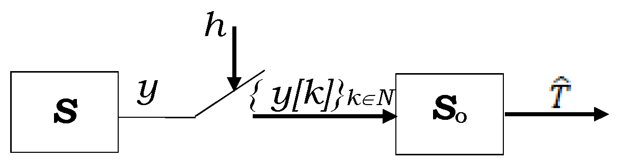
2.2. Discrete-Time Observer for Determining the Variation in the Parameters of a First-Order Continuous-Time System from Its Sampled Free Regime

In this section, we refer to the situation when the output of system S in Figure 1 is not available as a continuous-time signal y(t), but as a discrete-time signal ${\left\{y\left[k\right]\right\}}_{kϵN}$according to Equation (21) and Figure 5, where h is a constant sampling time:

$${\left\{y\left[k\right]\right\}}_{kϵN}, y_k=y\left(k·h\right).$$

(21)

Two possibilities for approximating the variation in T may be considered:

• Interpolation of the signal (21) followed by the processing of the interpolated signal with the PO from Figure 2
• Replacing the continuous-time PO with a homologous PO in discrete-time.

Due to the great computational effort associated with interpolation with continual smooth functions, only the second approach is of practical interest.

For the case in Figure 5, when the observer S₀ is a discrete-time system, we considered that the tracking subsystem results from the replacement in Equations (6), (8) and (9) of the integration and derivation operations according to Euler’s method and the backward difference, respectively [30]. Thus, for a constant sampling period h, we obtain, respectively:

$$\widehat{z}\left[k\right]=\widehat{z}\left[k-1\right]+h·\widehat{c}\left[k\right], \widehat{z}\left[0\right]={\widehat{z}}_0,$$

(22)

$$\epsilon \left[k\right]=z\left[k\right]-\widehat{z}\left[k\right],$$

(23)

$$\widehat{c}\left[k\right]=K_p\left(\epsilon \left[k\right]-\epsilon \left[k-1\right]\right)+h·K_i·\epsilon \left[k-1\right]+\widehat{c}\left[k-1\right], \widehat{c}\left[0\right]={\widehat{c}}_0 .$$

(24)

In (23) we have

$$z\left[k\right]=\ln \left(y_I\left[k\right]\right).$$

(25)

Equation (22) corresponds to block M in Figure 6, and Equation (24) to block TC.

Finally, instead of Equation (7), we will operate with Equation (26) and the average value (27):

$$\widehat{T}\left[k\right]=-\frac{1}{\widehat{c}\left[k\right]},$$

(26)

$${\widehat{T}}_m\left[k\right]=\frac{1}{k·h-k_0·h}·{\sum }_{k_0+1}^k\widehat{T}\left[k\right],k=k_0+1, k_0+2,\dots .$$

(27)

Here, $k_0$ corresponds to the time t₀ from which the average value is calculated. It is chosen so that the average value is not calculated over the time interval when the mentioned transient regime occurs.

The input signal (19) sampled with h = 5·10⁻⁶ s was used to validate the discrete-time PO. The results are shown in Figure 7. On the left are the input signal and the corresponding estimated signal. After a short-term transient regime, the follow-up is carried out without issue. According to the error {ε[𝑘]} represented in Figure 7b, the transient regime lasts about 2·10⁻³ s. On the right is illustrated $\left\{{\widehat{T}}_m\left[k\right]\right\}$. Ignoring the transient regime, the result practically coincides with that in Figure 4c. In (27) k₀ = 0 corresponds to t₀ = 10⁻³ s.

Additionally, for the validation of the discrete-time PO, we used the input signal (28) with a time constant which for t = 4·10⁻³ s has a jump from the value T₁ = 5.8·10⁻³ s to the value T₂ = 2.9·10⁻³ s.

y(t) = min {20·e^{−500·ln(2)·t},10·e^{−250·ln(2)·t}}.

(28)

The signal’s sampling period was h = 5·10⁻⁶ s. The results are shown Figure 8. Figure 8a illustrates the signal y(t) and the estimated signal $\left\{\widehat{y}\left[k\right]\right\}$, and Figure 8b the estimated variation $\left\{\widehat{T}\left[k\right]\right\}$. Note that the tracking is performed very well after going through a transient regime with an approximate duration of 0.25·10⁻³ s.

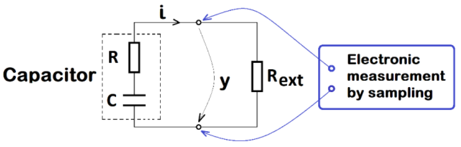
2.3. Method for Estimating the Parameters of a Capacitor

The process we refer to occurs in the circuit in Figure 9 and consists of discharging a real capacitor through an ideal resistor R_ext. In the R-C model used for the capacitor, R represents the ESR. The voltage at the terminals of the capacitor is y, and the discharging current i.

As a working hypothesis, we consider that both C and R vary in time, resulting in the so-called “circuit time constant T” being the function of time (29):

T(t) = C(t)⋅[R(t) + R_ext].

(29)

We also consider that $y\left(0\right)=y_0>0$. Under these circumstances, the discharging process is described by the model (1). Assuming the measurement of y(t) by sampling, the situation is identical to that described in Section 2.2. Consequently, we can determine the signal ${\left\{\widehat{T}\left[k\right]\right\}}_{k\in N}$ using the tracking subsystem (22)–(24), the linking Formulas (25) and (26), and the variation ${\left\{{\widehat{T}}_m\left[k\right]\right\}}_{k\in N}$ by Formula (27).

Given that for the sampling instants (29) becomes $T\left[k\right]=C\left[k\right]·\left(R\left[k\right]+R_{ext}\right)$, we can consider that beginning at the end of the transient regime, Equation (30) is valid:

$$\widehat{T}\left[k\right]=C\left[k\right]·\left(R\left[k\right]+R_{ext}\right).$$

(30)

Since, as will be seen below, ${\left\{\widehat{T}\left[k\right]\right\}}_{k\in N}\ne const.$, this result highlights that T varies during the discharging process. Naturally, we are interested in the variations ${\left\{C\left[k\right]\right\}}_{k\in N}$ and ${\left\{R\left[k\right]\right\}}_{k\in N}$. Their determination from a single Equation (30) is impossible because at each moment k⋅h, Equation (30) presents two unknown values. Hence, a second equation is needed, and that means a new capacitor’s discharge from the same initial condition y₀ through a different external resistance. However, this implies a process for which the dynamics at time k⋅h are characterized by a different pair $(C\left[k\right],$ $R\left[k\right])$.

For this reason, the only calculation alternative for the presented situation is the operation with equivalent values ${\widehat{T}}_e, {\widehat{C}}_e, {\widehat{R}}_e$ of the variations of $T, C, R$ linked by Equation (31):

$${\widehat{T}}_e={\widehat{C}}_e·\left({\widehat{R}}_e+R_{ext}\right),$$

(31)

and splitting the discharging process into at least two stages during which ${\widehat{C}}_e$ and ${\widehat{R}}_e$ can be considered constant. Let us admit in this context the possibility of performing the discharge of the same capacitor in two stages through two different external resistors, R_ext1 and R_ext2, assigned for each stage. As a consequence, the value of ${\widehat{T}}_e$, changes for the first and second stage to ${\widehat{T}}_{e1}$ and ${\widehat{T}}_{e2}$, respectively, and we obtain the system of Equation (32) with respect to ${\widehat{C}}_e$ and ${\widehat{R}}_e$:

$$\{\begin{array}{c}{\widehat{T}}_{e1}={\widehat{C}}_e·\left({\widehat{R}}_e+R_{ext1}\right)\\ {\widehat{T}}_{e2}={\widehat{C}}_e·\left({\widehat{R}}_e+R_{ext2}\right)\end{array}.$$

(32)

The above-described situation can be implemented with a good approximation using the discharging scheme in two stages, as shown in Figure 10a. At t_s, at the end of the first stage, the switch closes, determining the voltage variation y(t) presented in Figure 10b. This is due to the variation in the equivalent resistance R_ext with its different values, R_ext1 and R_ext2, according to Equation (33):

$$R_{ext1}=R_L , R_{ext2}=\frac{R_L·R_a}{R_L+R_a} .$$

(33)

The idea of modifying the value of the discharging resistor during the process appears in [6], which also shows the modification of the discharging resistor by connecting additional resistors in parallel.

2.4. Bisector Method

Assuming the validity of Equations (32) and (33), it is necessary to establish a method for determining the value of ${\widehat{T}}_e$. For this purpose, we consider the examples in Figure 11a where the curve ${\widehat{T}}_m\left(t\right)$ corresponds to the 220 µF/25 V electrolytic capacitor investigated in [29]. Due to the multiple oscillations, the variations in $\widehat{T}\left(t\right)$ would make it difficult to obtain an equivalent value. However, the variations in the average value ${\widehat{T}}_m$ are suitable for defining an equivalent value. Given that at the end of the discharging process, the signal-to-noise ratio ends up affecting the recorded values of the voltage y(t) we adopt, in the following, as an equivalent value of T_e, the value of ${\widehat{T}}_m$ corresponds to the moment t₁ when the Equation (34) is fulfilled:

$${\widehat{T}}_m\left(t_1\right)=t_1-t_0.$$

(34)

Graphically, Equation (34) has the following interpretation:

$${\widehat{T}}_e={\widehat{T}}_m\left(t_1\right)=AC=BC.$$

(35)

3. Results

The output electrolytic capacitor of a DC–DC buck converter was considered as an example to apply the PO and the method for calculating the capacitor’s equivalent parameters using the PO. Section 3.1 presents the experimental context, and Section 3.2 the outcome results.

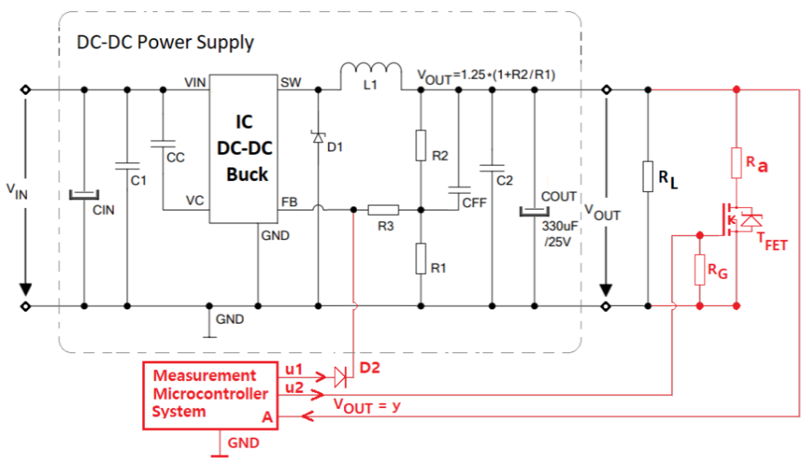
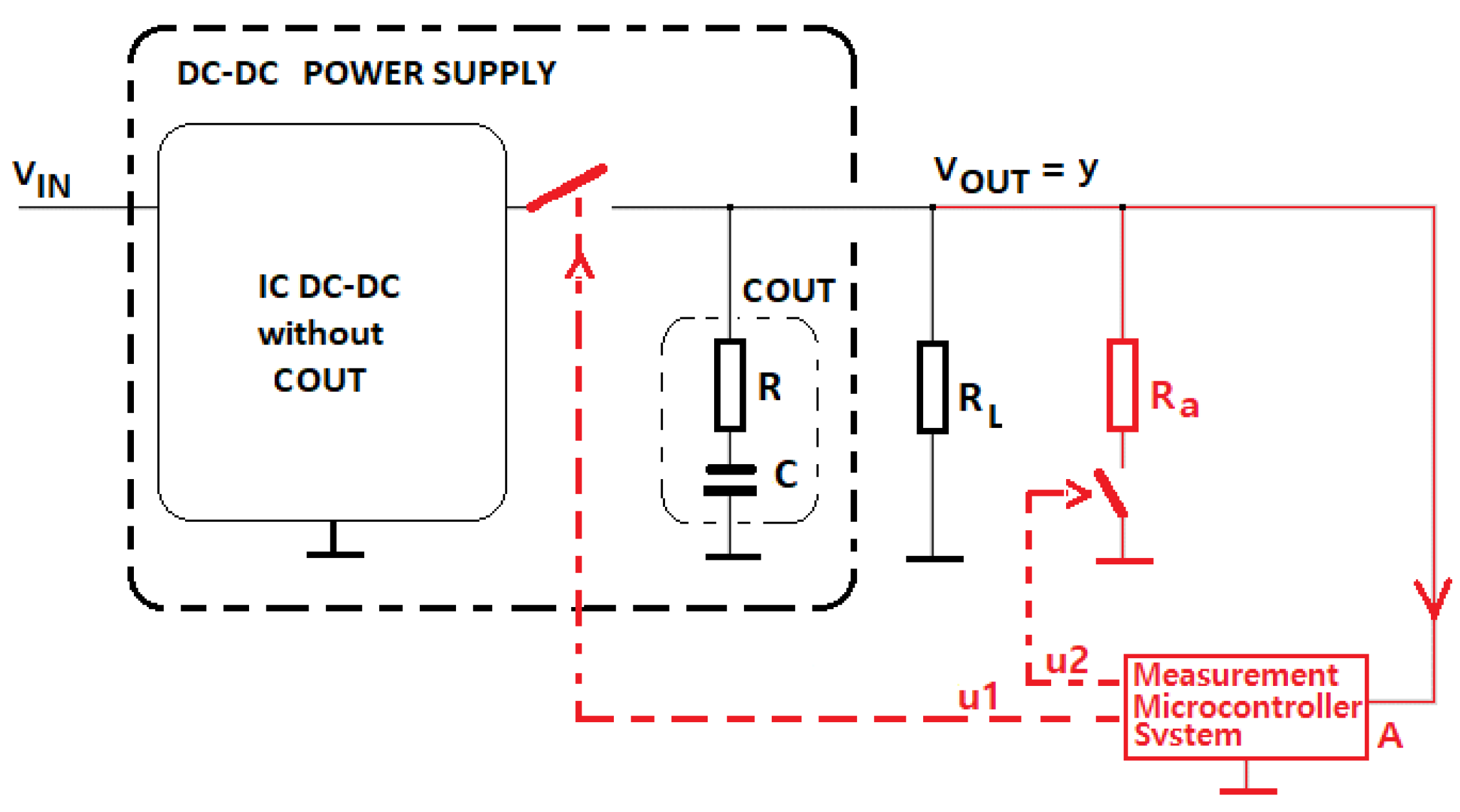
3.1. The Circuit Used to Estimate the Parameters of the Output Capacitor of a DC–DC Buck Converter

The discrete-time PO is further used to determine the equivalent parameters of the COUT electrolytic capacitor of the DC–DC buck converter in Figure 12 [31]. The power supply is realized with a dedicated integrated circuit. At the input of the source, the unstabilized voltage V_IN is used, and at the output, the stabilized voltage V_OUT (V_OUT < V_IN) is applied to load R_L. The elements and connections represented in red were added to produce a non-invasive two-stage discharge. The signal u1, applied by an ATMEGA 328 microcontroller, on the FB pin of the integrated circuit (IC DC–DC Buck) via diode D2, stops the DC–DC power supply and triggers the first stage of the discharging process. The microcontroller also controls by u2 signal the T_FET transistor to connect at the proper moment the additional resistor R_a. The signal applied to input A is used to monitor the voltage V_OUT = y, determining by its level the moment when the second stage must be initiated. For applications, the value of COUT can be adopted in a wide range. Thus, compared with the capacitor of 330 µF in Figure 12, we used two capacitors of 100 µF and 470 µF. For the values of R1, R2, C2 and CFF we used 270 Ω, 4.05 kΩ, 100 nF and 10 nF, respectively.

Assuming that the elements connected before the COUT do not practically influence the process of discharging the COUT through the load resistor, the diagram in Figure 12 can be simplified as in Figure 13.

The signals u1 and u2 are time-delayed pulses: a high level on u1 stops the DC–DC buck converter and triggers the first stage (discharging of the COUT capacitor through the load R_L), and a high level on u2, generated at t_s seconds after u1, connects the additional resistor R_a in parallel with R_L. The moment t_s corresponds to the instant when y reaches a preset threshold level. The discharge of the COUT capacitor is represented in Figure 10b. Equation (36) resulting from Equation (32) is valid:

$${\widehat{C}}_e=\frac{{\widehat{T}}_{e1}-{\widehat{T}}_{e2}}{R_L^2/\left(R_L+R_a\right)} , {\widehat{R}}_e=R_L·\left[\frac{{\widehat{T}}_{e1}·R_L}{\left({\widehat{T}}_{e1}-{\widehat{T}}_{e2}\right)·\left(R_L+R_a\right)}-1\right].$$

(36)

3.2. Experimental Results

The experiments were performed for two cases in which the COUT capacitor in Figure 12 and Figure 13 had the nominal values of 100 μF and 470 μF, respectively. The capacitors were of the type aluminium electrolytic capacitor Nichicon 100 μF/25 V and Panasonic polymer SMD electrolytic capacitor 470 μF/25 V, respectively. The discharges were performed each time in two stages through the resistors with the resistances R_L = 29.89 Ω and R_a = 15.84 Ω while the setup environment temperature was constant 22 °C. The voltage across the output capacitor terminals was measured using a LeCroy WaveSurfer 104MX digital oscilloscope (8-bit resolution) and saved in files for offline digital processing in the MATLAB-SIMULINK environment. The sampling frequency of the oscilloscope was several times higher than the corresponding frequency bandwidth of the capacitor discharging process according to the oversampling technique. Thus, we took measurements with a sampling frequency of 5 MHz. The results are shown in Figure 14, Figure 15, Figure 16 and Figure 17 that refer to the use of the method in Section 2.2. The resolutions indicated in the texts of Figure 14 and Figure 17 are for information only.

Figure 14 shows the discharging curve stages of the 100 μF capacitor, together with the estimates calculated with the discrete-time PO. Figure 14a corresponds to the first stage, while Figure 14b to the second stage. Figure 15 illustrates for the first stage the variations $\widehat{T}\left(t\right)$ and ${\widehat{T}}_m\left(t\right)$ calculated in two processing hypotheses. Thus, Figure 15a,b corresponds to the processing of the measured voltage values filtered with the 51-point moving average filter (38), while Figure 15c,d corresponds to unfiltered data processing.

$$y_{av}\left[n\right]=\frac{1}{51}·{\sum }_{j=n-25}^{n+25}x\left[n-j\right].$$

(37)

Figure 15b,d shows, using the bisector method, the equivalent values ${\widehat{T}}_{e1}=2.9066·{10}^{-3} \mathrm{s}$ and ${\widehat{T}}_{e1}=2.9071·{10}^{-3} \mathrm{s}$. The calculated values correspond to t₁ = 3.6087⋅10⁻³ s, and t₁ = 3.6137⋅10⁻³ s. Therefore, we consider that:

$${\widehat{T}}_{e1}=2.9·{10}^{-3} \mathrm{s}.$$

(38)

Figure 16 shows the counterparts of Figure 15 for the second discharging stage. The equivalent values calculated for filtered (Figure 16a) and unfiltered (Figure 16c) records are ${\widehat{T}}_{e2}=1.1024·{10}^{-3} \mathrm{s}$, (Figure 16b) and ${\widehat{T}}_{e2}=1.1036·{10}^{-3} \mathrm{s}$ (Figure 16d), respectively. They correspond to the moments t₁ = 3.6137·10⁻³ s and t₁ = 2.1036·10⁻³ s, respectively. Here, we will consider:

$${\widehat{T}}_{e2}=1.1·{10}^{-3} \mathrm{s}.$$

(39)

For the values in (38) and (39), the Formula (36) also leads to equivalent values

$${\widehat{C}}_e=92.84·{10}^{-6} F, {\widehat{R}}_e=1.5339 \Omega .$$

(40)

In the case of the capacitor with a nominal value of 470 µF, the two discharging stages are shown in Figure 17a,b, respectively.

From calculations similar to those of the 100 μF capacitor, we obtained ${\widehat{T}}_{e1}=13.5·{10}^{-3} \mathrm{s}$ and ${\widehat{T}}_{e2}=4.9·{10}^{-3} \mathrm{s}$, respectively:

$${\widehat{C}}_e=443.6·{10}^{-6} F, {\widehat{R}}_e=0.7324 \Omega .$$

(41)

4. Discussion

The purpose of this article is first of all theoretical. The proposed POs were used in analytical examples and for experimental data regarding the electrolytic capacitor COUT in Figure 12 and Figure 13. For both capacitors tested (100 μF/25 V and 470 μF/25 V), the experimental data were processed using the discrete-time PO.

The main aspects that we retain from the study are summarized below in points 1–7. The figures and/or the equations that support these aspects are specified in brackets.

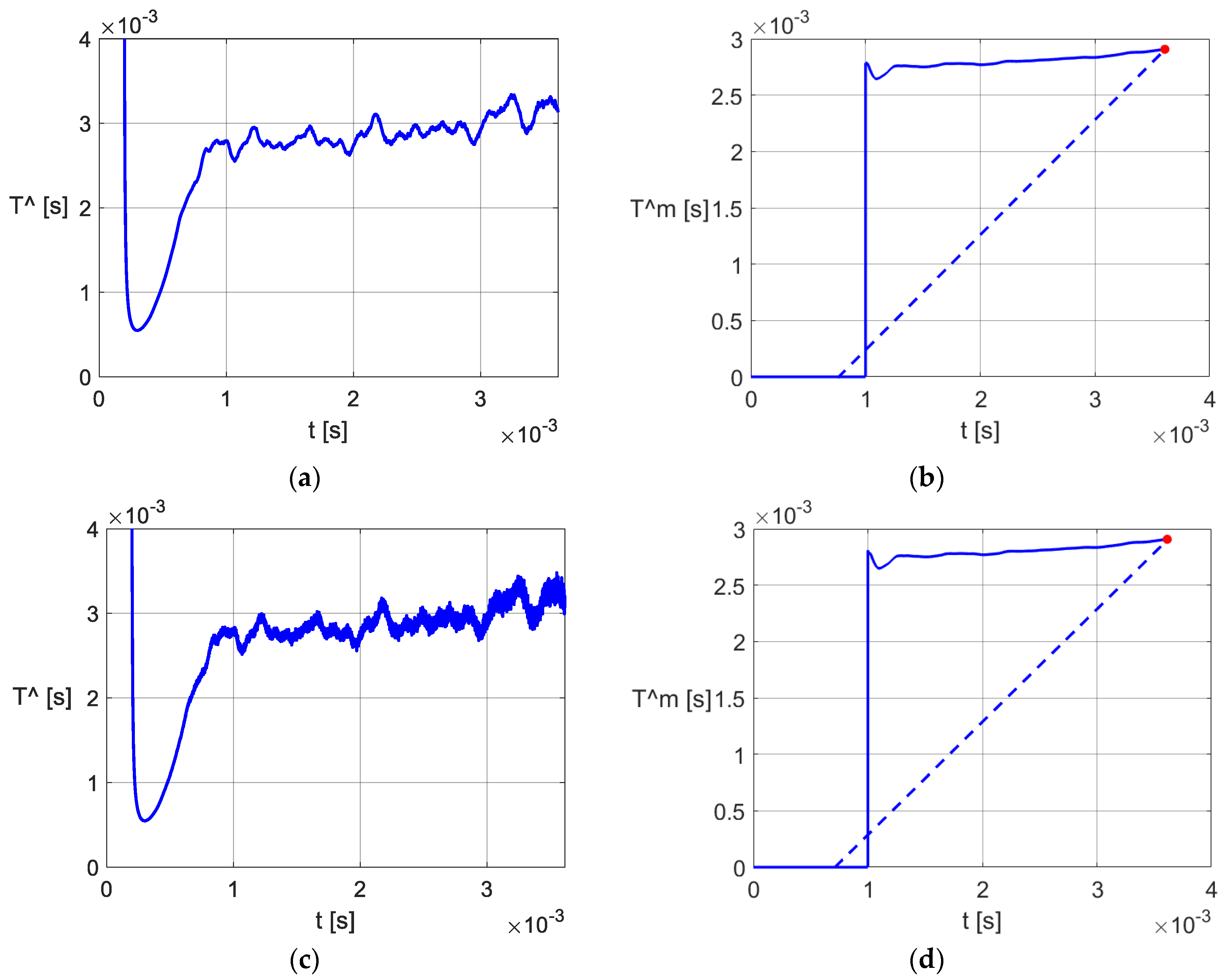
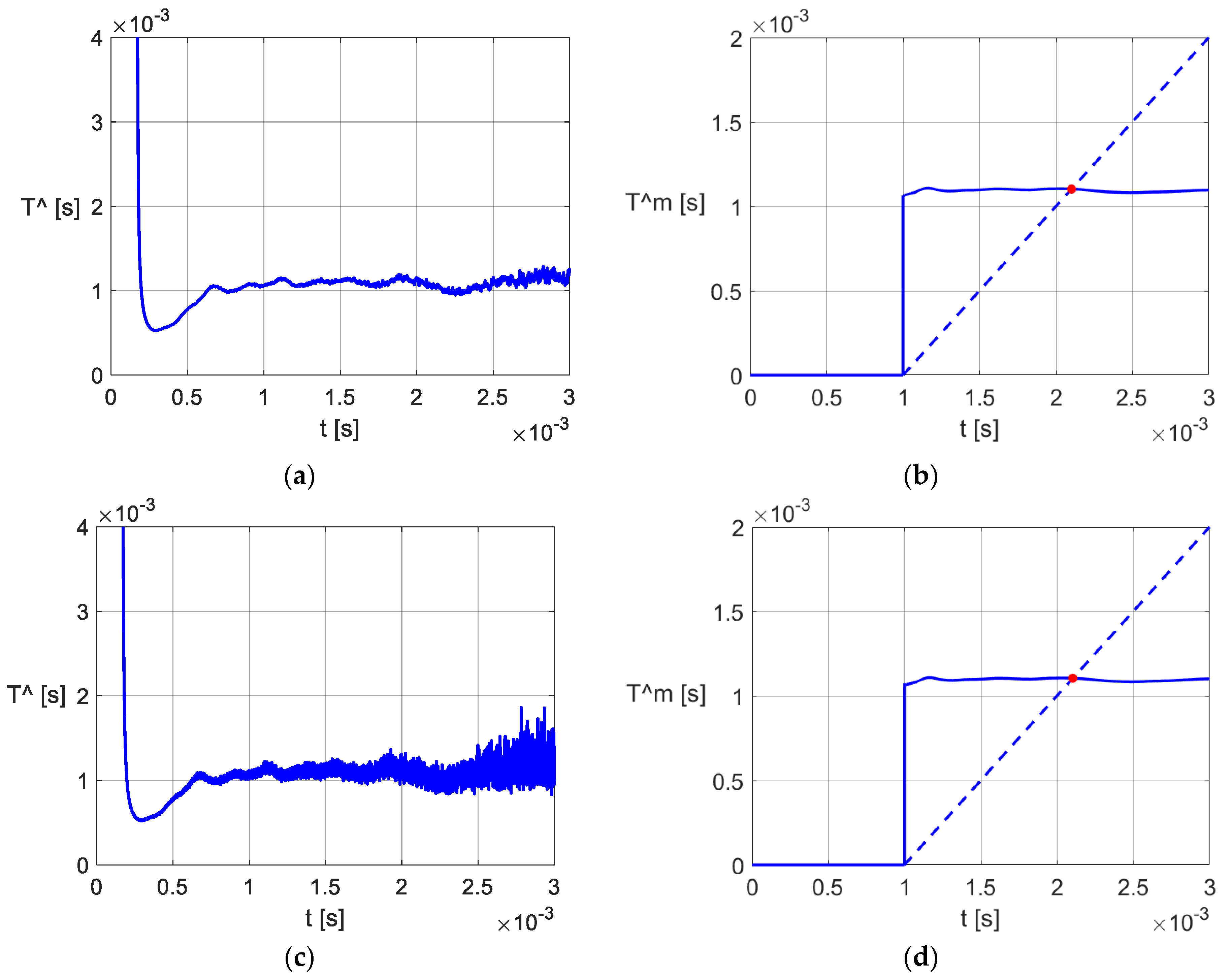
• During the capacitor’s discharging process, the parameter T of the circuit, currently called the time constant, varies (Figure 15a,c and Figure 16a,c). According to [19], the variation in the estimated value $\widehat{T}{\left(t\right)}_{ }$ reflects that both C and ESR vary in time. From a practical perspective, this conclusion implies the defining of equivalent values: ${\widehat{T}}_{e, }{\widehat{C}}_e,{\widehat{R}}_e.$ To determine the equivalent value ${\widehat{T}}_e$ of T(t), the variation in the average value $\left\{{\widehat{T}}_m\left[k\right]\right\}$ was calculated using the discrete-time PO, and ${\widehat{T}}_e$ was extracted by the “bisector method” (Figure 11, Figure 15b,d and Figure 16b,d).
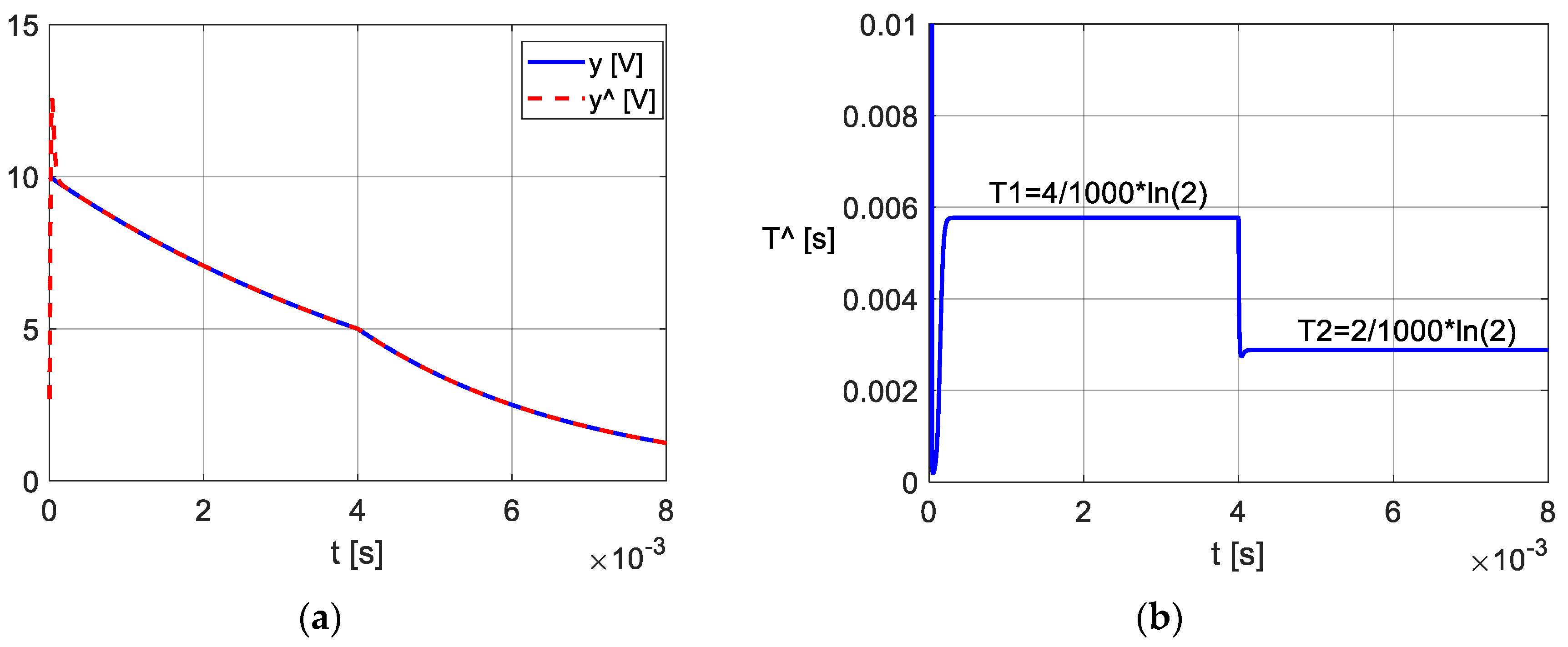
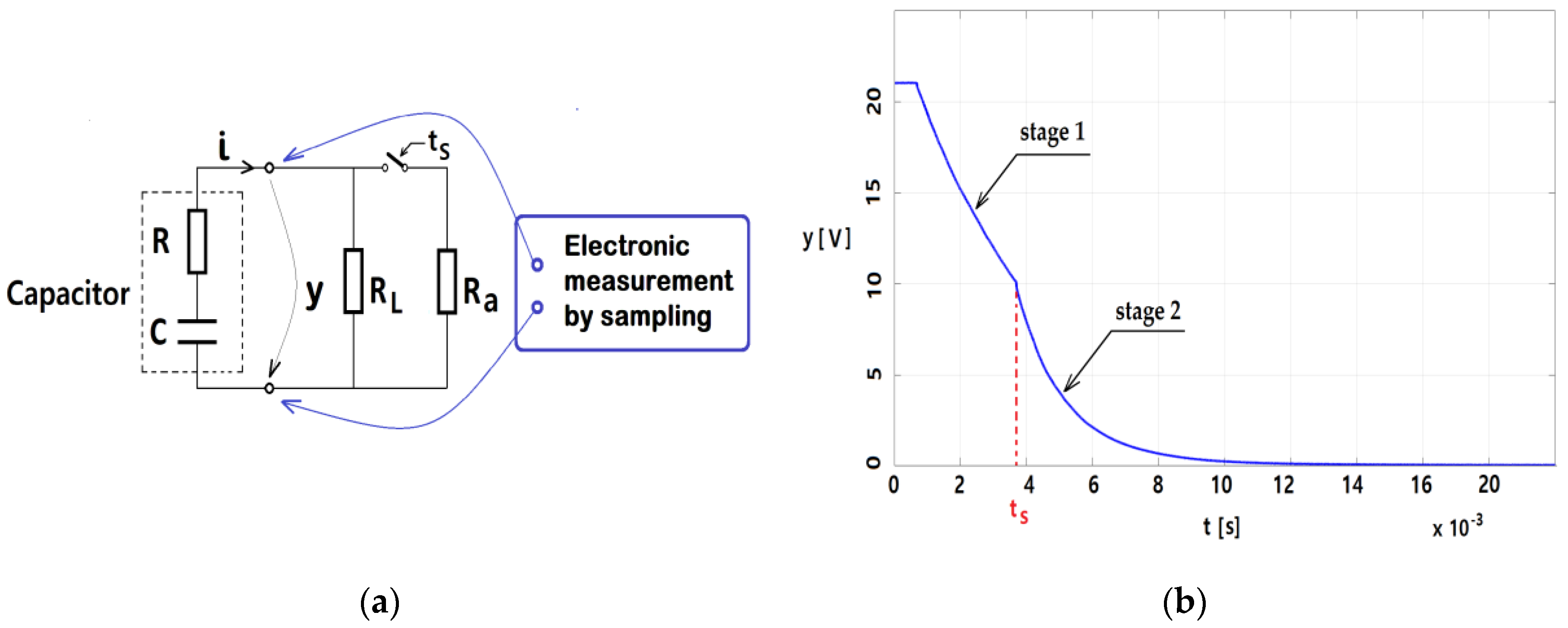
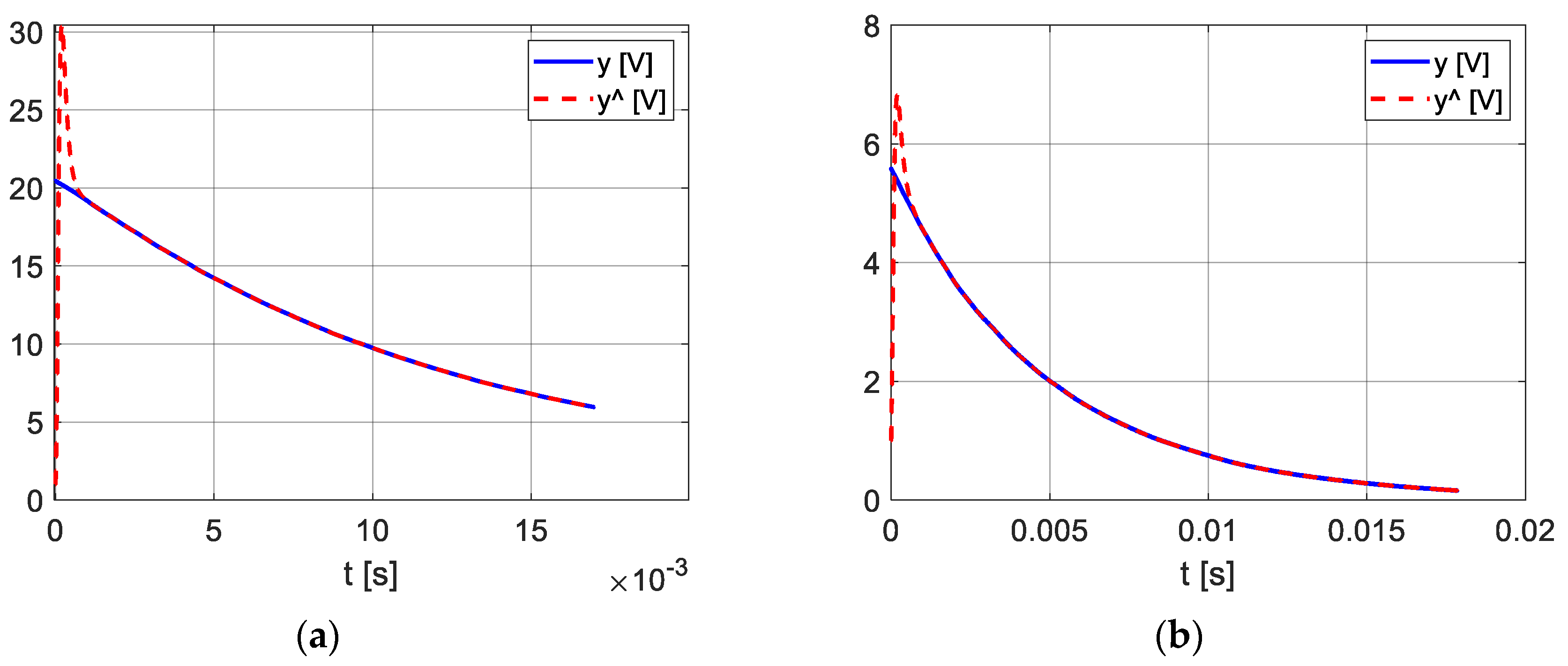
• The working hypothesis of simplifying the scheme in Figure 12 as in Figure 13 means that the discharge current on the left side of COUT is negligible with respect to the discharge current on the right side. The hypothesis is confirmed by simulation with a Simscape Electrical model.
• Obtaining the values ${\widehat{C}}_e,{\widehat{R}}_e$ requires two discharging experiments. To maintain, as far as possible, the same discharging regime, according to the method presented in [6] a two-stage discharge was used (Figure 10). For each capacitor, the two stages were treated separately (Figure 15 and Figure 16). As the time required for the two discharge steps is much longer than the ripple’s discharge time, the method can be applied as in [6], only when the converter is stopped. Unlike [6], where the capacitor discharge process exceeds 10 s, in our paper the discharge time is less than 0.02 s. As a result, the necessary stop time of the converter is quite short. The difference is due to the inertia of the discharging electrical circuits to which the capacitors belong.
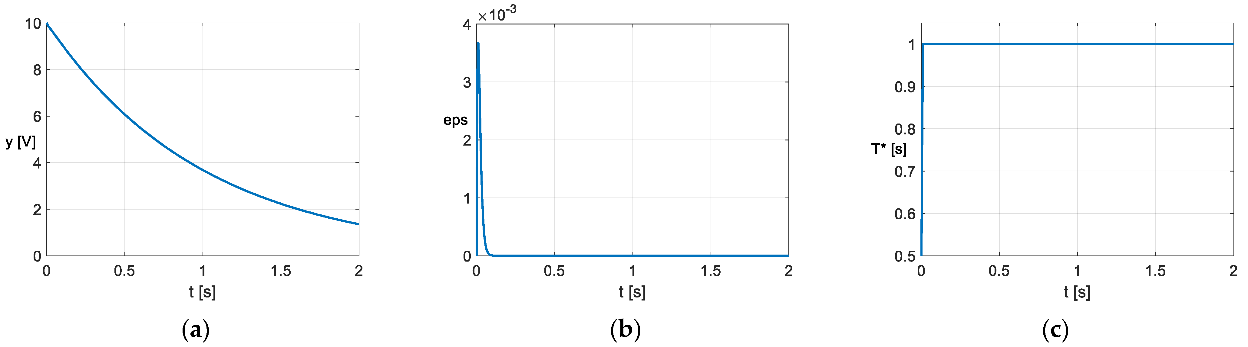
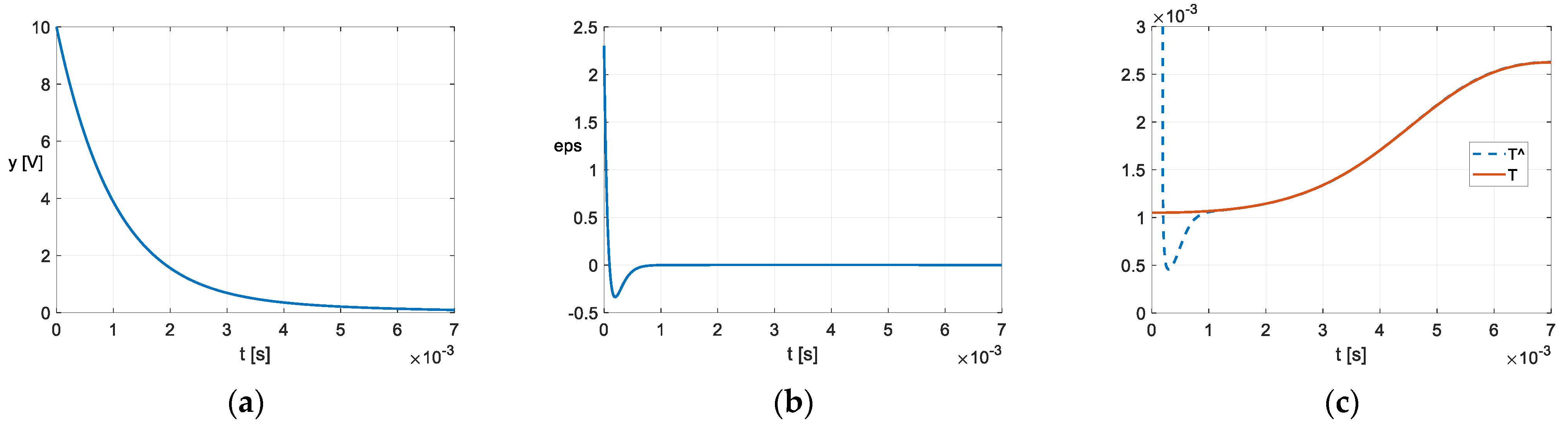
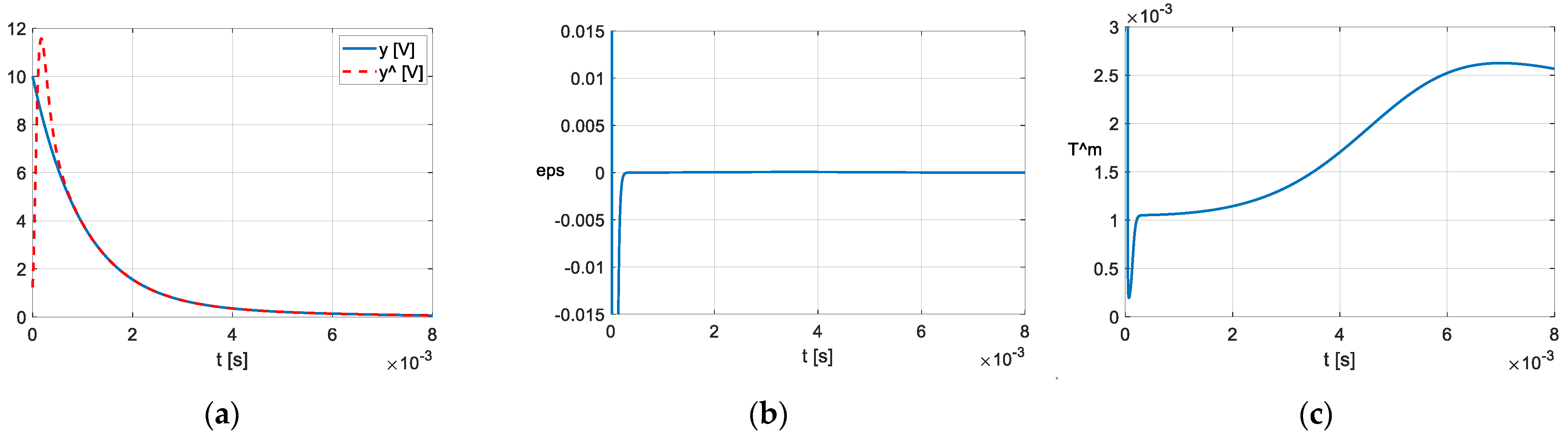
• The estimation of the T parameter with both proposed POs is affected at the beginning by a short transient regime caused by the inconsistency between the initial state variables of the PO with the observer’s input. The duration of the transient may be shortened by appropriately adopting the parameters of the observer. As the transient cannot be eliminated, it was avoided in the calculation of ${\widehat{T}}_m\left(t\right)$ by choosing the moment t₀. The attenuation time of the estimation error of the PO used for the experimental data is a maximum of 10⁻³ s (Figure 14 et seq.), and so is smaller than the attenuation of approx. 5·10⁻³ s that occurred in [3], and much smaller than that of approx. 50·10⁻³ s that occurred in [27,28].
• The study of the influence of noise filtering on $\widehat{T}\left(t\right)$, applied for 100 μF, does not show favorable noticeable consequences on the equivalent value ${\widehat{T}}_e$ (Figure 16b,d).
• In the theoretical examples, for which the values of T(t) can be verified analytically, the PO ensures the correct estimation of T after the attenuation of the transient regime (Figure 3, Figure 4, Figure 7 and Figure 8). Since a theoretical verification of T(t) is impossible in the practical case of the two capacitors, we analysed the equivalent values (40) and (41). Both values of ${\widehat{C}}_e$ are in the range of 20 Hz–25 kHz of the measured frequency characteristics C(f), while the values of ${\widehat{R}}_e$ are below 20 Hz. It should be also noted that the calculated values of ${\widehat{R}}_e$ with Formula (36) are very sensitive in relation to the values of ${\widehat{T}}_{e1}-{\widehat{T}}_{e2}$, R_L and R_a, while the values of ${\widehat{C}}_e$ are less sensitive.
• The recording resolution, as shown in Figure 14, Figure 15 and Figure 17, in relation to the dynamics of the capacitor’s discharge process, should not lead to the conclusion that the use of PO requires a high sampling frequency or oversampling. Indeed, the calculated values of ${\widehat{T}}_e$ have undergone non-essential changes using a set of measured sequences $\left\{\left(t_i,y_i\right)\right\}$, corresponding to a sampling period of 20 μs from the discharge curves in Figure 16. This result, in conjunction with the simplicity of the PO algorithm, expands the potential of the POs for real-time implementation.

5. Conclusions

This paper proposes a parameter observer designed to estimate the time constant of a first-order linear system in a free regime. The estimation, performed on the basis of the variation in the system’s output, is possible also when this parameter is time-variable.

The observer can be used for electrolytic capacitors for which the parameters are time-varying during transient processes. This is highlighted by discharging the capacitor through a resistor, and considered for the capacitor the equivalent R-C serial scheme. Since the voltage across the capacitor terminals is experimentally obtained in sampled form, the discrete time version of the observer is recommended. From the voltage curve generated for two-stage discharges, equivalent values for the parameters of the R-C serial scheme are determined using a processing procedure/algorithm with few operations. The procedure is applied in the paper to determine the equivalent parameters of the output capacitor of a DC–DC buck converter. Two capacitors with different nominal values are considered for the same converter scheme. The results obtained via offline processing support the general possibility of determining equivalent parameters for capacitors by using the parameter observers. The tracking process of the time constant variation is performed practically after approx. 10⁻³ s. The obtained values for the equivalent capacitance are according to the spectral range of the discharge signal, while the values for the equivalent resistance belong to the range below 20 Hz.

Due to the simplicity of the working algorithm, the parameter observer can be integrated for the condition monitoring of capacitors in maintenance and fault detection applications. As the observer is designed for first-order linear processes, its application should not be restricted to the area of electrolytic capacitors.

References

1. Wang, H.; Blaabjerg, F. Reliability of capacitors for DC-link applications in power electronic converters—An overview. IEEE Trans. Ind. Appl. 2014, 50, 3569–3578. [Google Scholar] [CrossRef] [Green Version]
2. Wang, H.; Ma, K.; Blaabjerg, F. Design for reliability of power electronic systems. In Proceedings of the IECON 2012—38th Annual Conference on IEEE Industrial Electronics Society, Montreal, QC, Canada, 25–28 October 2012; pp. 33–34. [Google Scholar]
3. Cen, Z.; Stewart, P. Condition parameter estimation for photovoltaic buck converters based on adaptive model observers. IEEE Trans. Reliab. 2017, 66, 148–160. [Google Scholar] [CrossRef]
4. Laadjal, K.; Bento, F.; Jlassi, I.; Cardoso, A.J.M. Online Condition Monitoring of Electrolytic Capacitors in DC-DC Interleaved Boost Converters, Adopting a Model-Free Predictive Controller. In Proceedings of the 2021 IEEE 15th International Conference on Compatibility, Power Electronics and Power Engineering (CPE-POWERENG), Florence, Italy, 14–16 July 2021. [Google Scholar]
5. Khandebharad, A.R.; Dhumale, R.B.; Lokhande, S.S.; Lokhande, S.D. Real time remaining useful life prediction of the electrolytic capacitor. In Proceedings of the 2015 International Conference on Information Processing (ICIP), Pune, India, 16–19 December 2015; pp. 631–633. [Google Scholar]
6. Wu, Y.; Du, X. A VEN Condition Monitoring Method of DC-Link Capacitors for Power Converters. IEEE Trans. Ind. Electron. 2019, 66, 1296–1306. [Google Scholar] [CrossRef]
7. Zhao, Z.; Davari, P.; Lu, W.; Wang, H.; Blaabjerg, F. An Overview of Condition Monitoring Techniques for Capacitors in DC-Link Applications. IEEE Trans. Power Electron. 2021, 36, 3692–3716. [Google Scholar] [CrossRef]
8. Zhao, Z.; Lu, W.; Davari, P.; Du, X.; Iu, H.H.C.; Blaabjerg, F. An Online Parameters Monitoring Method for Output Capacitor of Buck Converter Based on Large-Signal Load Transient Trajectory Analysis. IEEE J. Emerg. Sel. Top. Power Electron. 2021, 9, 4004–4015. [Google Scholar] [CrossRef]
9. Gupta, Y.; Ahmad, M.W.; Narale, S.; Anand, S. Health Estimation of Individual Capacitors in a Bank with Reduced Sensor Requirements. IEEE Trans. Ind. Electron. 2019, 66, 7250–7259. [Google Scholar] [CrossRef]
10. Corti, F.; Reatti, A.; Patrizi, G.; Ciani, L.; Catelani, M.; Kazimierczuk, M.K. Probabilistic evaluation of power converters as support in their design. IET Power Electron. 2020, 13, 4542–4550. [Google Scholar] [CrossRef]
11. Yao, B.; Chen, H.; Hi, X.-Q.; Xiao, Q.-Z.; Kuang, X.-J. Reliability and failure analysis of DC/DC converter and case studies. In Proceedings of the 2013 International Conference on Quality, Reliability, Risk, Maintenance, and Safety Engineering (QR2MSE), Chengdu, China, 15–18 July 2013; pp. 1133–1135. [Google Scholar]
12. Bindi, M.; Corti, F.; Grasso, F.; Luchetta, A.; Manetti, S.; Piccirilli, M.-C.; Reatti, A. Failure prevention in DC-DC converters: Theoretical approach and experimental application on a Zeta converter. In IEEE Transactions on Industrial Electronics (Early Access); IEEE: Piscataway, NJ, USA, 2022. [Google Scholar] [CrossRef]
13. Duan, X.; Zou, J.; Li, B.; Wu, Z.; Lei, D. An Online Monitoring Scheme of Output Capacitor’s Equivalent Series Resistance for Buck Converters without Current Sensors. IEEE Trans. Ind. Electron. 2021, 68, 10107–10117. [Google Scholar] [CrossRef]
14. Ren, L.; Gong, C.; Zhao, Y. An Online ESR Estimation Method for Output Capacitor of Boost Converter. IEEE Trans. Power Electron. 2019, 34, 10153–10165. [Google Scholar] [CrossRef]
15. Gasperi, M.L. Life prediction modeling of bus capacitors in AC variable frequency drives. In Proceedings of the IEEE Conference Record of Annual Pulp and Paper Industry Technical Conference, Jacksonville, FL, USA, 20–23 June 2005; pp. 141–146. [Google Scholar]
16. Plazas-Rosas, R.A.; Orozco-Gutierrez, M.L.; Spagnuolo, G.; Franco-Mejía, É.; Petrone, G. DC-Link Capacitor Diagnosis in a Single-Phase Grid-Connected PV System. Energies 2021, 14, 6754. [Google Scholar] [CrossRef]
17. Ahmeid, M.; Armstrong, M.; Gadoue, S.; Al-Greer, M.; Missailidis, P. Real-time parameter estimation of DC-DC converters using a self-tuned kalman filter. IEEE Trans. Power Electron. 2017, 32, 5666–5674. [Google Scholar] [CrossRef] [Green Version]
18. Soliman, H.; Wang, H.; Blaabjerg, F. A Review of the Condition Monitoring of Capacitors in Power Electronic Converters. IEEE Trans. Ind. Appl. 2016, 52, 4976–4989. [Google Scholar] [CrossRef]
19. Barbulescu, C.; Dragomir, T.-L. Parameter estimation for a simplified model of an electrolytic capacitor in transient regimes. J. Phys. Conf. Ser. 2021, 2090, 012143. [Google Scholar] [CrossRef]
20. Li, L.; Yao, K.; Guan, C.; Wu, C.; Fang, B.; Zhang, Z.; Ma, C.; Chen, J.; Zhang, J. A quasi-online monitoring method of output capacitor and boost inductor for DCM boost converter. In Proceedings of the 2019 IEEE Energy Conversion Congress and Exposition (ECCE), Baltimore, MD, USA, 29 September–3 October 2019; pp. 2205–2211. [Google Scholar]
21. Luenberger, D. Introduction to Dynamic Systems. In Theory, Models, and Applications; John Wiley & Sons: New York, NY, USA, 1979. [Google Scholar]
22. Setoodeh, P.; Habibi, S.; Haykin, S. Nonlinear Filters: Theory and Applications; John Wiley & Sons: New York, NY, USA, 2022. [Google Scholar]
23. Radke, A.; Gao, Z. A survey of state and disturbance observers for practitioners. In Proceedings of the American Control Conference, Minneapolis, MN, USA, 14–16 June 2006; Volume 2006, pp. 5183–5188. [Google Scholar]
24. Gonzalez-Fonseca, N.; de Leon-Morales, J.; Leyva-Ramos, J. Observer-based controller for switch-mode dc-dc converters. In Proceedings of the 44th IEEE Conference on Decision and Control, Seville, Spain, 15 December 2005; pp. 4773–4778. [Google Scholar]
25. Levin, K.T.; Hope, E.M.; Domínguez-Garcíay, A.D. Observer-based fault diagnosis of power electronics systems. In Proceedings of the 2010 IEEE Energy Conversion Congress and Exposition, Atlanta, GA, USA, 12–16 September 2010; pp. 4434–4440. [Google Scholar]
26. Chowdhury, N.R.; Belikov, J.; Baimel, D.; Levron, Y. Observer-based detection and identification of sensor attacks in networked CPSs. Automatica 2020, 121, 109166. [Google Scholar] [CrossRef]
27. Jain, P.; Poon, J.; Jian, L.; Spanos, C.; Sanders, S.R.; Xu, J.X.; Panda, S.K. An improved robust adaptive parameter identifier for DC-DC converters using H-infinity design. In Proceedings of the 2018 IEEE Applied Power Electronics Conference and Exposition (APEC), San Antonio, TX, USA, 4–8 March 2018; pp. 2922–2926. [Google Scholar]
28. Meng, J.L.; Chen, E.X.; Ge, S.J. Online E-cap condition monitoring method based on state observer. In Proceedings of the 2018 IEEE International Power Electronics and Application Conference and Exposition (PEAC), Shenzhen, China, 4–7 November 2018; pp. 1–6. [Google Scholar]
29. Szidarovszky, F.; Bahill, A.T. Linear Systems Theory, 2nd ed.; Routledge: London, UK, 2018. [Google Scholar]
30. James, G. Advanced Modern Engineering Mathematics; Pearson Education Limited: London, UK, 2004. [Google Scholar]
31. Datasheet 5 A 180 KHz 36 V Buck DC to DC Converter XL4015. Available online: www.xlsemi.com (accessed on 26 April 2022).
Figure 1. The block diagram of the continuous-time observation structure of the parameter T.
Applsci 12 04891 g001
Figure 2. The structure of the parameter observer S0.
Applsci 12 04891 g002
Figure 3. The behavior of the PO for y(t) = 10 e t , z ^ 0 = 2.302585 , c ^ 0 = 2 , τ = 0.5   s , ω 0 = 100   s 1 , Kp = 200   s 1 , Ki = 10 , 000   s 2 : (a) input signal y(t); (b), error ε(t); (c) estimated time-constant.
Applsci 12 04891 g003
Figure 4. The behaviour of the PO for y(t) given by the Formula (19), z ^ 0 = 0 , c ^ 0 = 0 , τ = 10 3   s , ω 0 = 10 4   s 1 , Kp = 2⋅104 s 1 , Ki = 108 s 2 : (a) input signal y(t); (b) error ε(t); (c) estimated T ^ , and T calculated with (20).
Applsci 12 04891 g004
Figure 5. The block diagram of the observation of the parameter T.
Applsci 12 04891 g005
Figure 6. Block diagram of the discrete-time tracking subsystem.
Applsci 12 04891 g006
Figure 7. The estimation of the parameter { T ^ m [ k ] } k N in the case that the signal (19) is sampled: (a) the input signal; (b) the signal {ε[𝑘]}; (c) the estimated average value T ^ m .
Applsci 12 04891 g007
Figure 8. Estimation of the parameter { T [ k ] } k N for the sampled signal corresponding to (28): (a) the signal (28) and its estimate; (b) the estimated time constant.
Applsci 12 04891 g008
Figure 9. The analysed circuit.
Applsci 12 04891 g009
Figure 10. The two-stage discharging of a capacitor: (a) experimental scheme; (b) voltage variation at capacitor terminals during the two-stages.
Applsci 12 04891 g010
Figure 11. Calculation of T ^ e : (a) with the bisector method; (b) with the extension of the bisector method.
Applsci 12 04891 g011
Figure 12. Diagram for determining the transient equivalent values of the COUT capacitor parameters.
Applsci 12 04891 g012
Figure 13. Simplified representation of the diagram in Figure 12.
Applsci 12 04891 g013
Figure 14. Results obtained with the discrete-time PO for the two-stage discharge of the 100 µF capacitor. Recording resolution: 50 ns. (a) The first stage of discharge; (b) the second stage of discharge.
Applsci 12 04891 g014
Figure 15. The variations T ^ ( t ) and T ^ m ( t ) for the first discharging stage of the 100 μF capacitor in Figure 14a calculated using a discrete-time PO for: (a,b) filtered data; (c,d) unfiltered data.
Applsci 12 04891 g015
Figure 16. Variations T ^ ( t ) and T ^ m ( t ) calculated with the discrete-time PO for the second stage of discharge of 100 µF in Figure 14b: (a,b) the results calculated using filtered data; (c,d) results calculated using unfiltered data.
Applsci 12 04891 g016
Figure 17. Two-stage discharge of a 470 μF capacitor. Recording resolution: 200 ns. (a) The first discharging stage; (b) the second discharging stage.
Applsci 12 04891 g017
Publisher’s Note: MDPI stays neutral with regard to jurisdictional claims in published maps and institutional affiliations.