CFD Investigations of Cyclone Separators with Different Cone Heights and Shapes

Abstract

Due to the great achievements in the field of optimization of the design of cyclone separators, non-standard solutions are sought to increase their performance. Therefore, in this study, we consider the impact of different cone and cylinder height variants on the performance of cyclone separators. Additionally, we propose non-standard shapes for these sections. Three different heights: H/D = 0.5, 1.0, and 1.5, with D (the main cyclone body diameter), are analyzed. Since the cone is one of the most important geometrical entities, three different shapes viz. a straight (conventional) profile, a concave profile as well as a convex profile are also taken into account. Cyclone performance is rated at three different inlet velocities viz. U_in = 10 m/s, 15 m/s, and 20 m/s. Hence, a total of 27 simulations have been performed using the Reynolds stress model. It becomes apparent from the present study that the pressure loss is lowest in the convex variant, whereas the separation efficiency is better in the conventional design. Furthermore, an increase in the length of the cylindrical section reduces pressure drop with a mild decrease in the collection efficiency in all variants.

1. Introduction

Cyclone separators are mechanical separators that are used to remove the particulate matter contained in the gas stream. Due to tangential injection and the curved wall, the dust-laden gas experiences a swirling motion that generates a centrifugal force field readily felt by suspended solid particles. This causes the solid particles to move in a radially outward direction towards the walls, thereby aiding the separation process. Hence, the particle concentration near the walls is higher for larger particles, and these particles are transported down to the collection bin attached at the cyclone bottom under the influence of axial velocity [1]. Cyclones are used in almost every industry where the solid particles are to be separated before releasing the fluid into the open atmosphere. Cyclones are used either as pre-separators to reduce the dust loading on the bag filters or as a final separation unit. Other roles include the classification of particles according to the size to recover the catalyst and many more. These devices are popular due to several advantages such as significantly shorter particle residence time, simple construction, ability to operate continuously even in corrosive environments, lower maintenance cost, and no moving parts (to name a few) [2,3]. Cyclones find application in several industries such as steel plants, cement industries, flour mills, power plants, etc. [4].

Since the development of cyclone separators, several studies have been undertaken to optimize the construction of these separators. The vortex finder diameter significantly affects the performance of cyclone separators—with an increase in diameter of the vortex finder, the pressure drop largely reduces, followed by a net reduction in the collection efficiency [5,6] and vice-versa. The insertion length of the outlet tube mildly influences the cyclone performance [7,8]. The eccentricity provided to the centre of the outlet tube largely affects the cyclone performance [9]. If performed without special care, the cyclone performance may deteriorate; hence, this aspect requires performing an optimization before implementation [10]. The vortex finder with cross-shaped blades decreases the pressure drop by more than 16% with a slight improvement of 0.64% in the separation efficiency [11]. Installing the de-swirler closer to the vortex finder inlet counts more on cyclone performance [12]. The convergent-divergent vortex finder helped to improve the pressure drop by as much as 6% followed by a reduction in the cut size from 1.6 µm to 1.4 µm [13]. The main cyclone body diameter (D) significantly influences the performance—an increase in the cyclone main body diameter increases the pressure drop, whereas the collection efficiency of larger particles is improved [14,15]. The increase in the length of cyclones plays a vital role; in fact, this is the only parameter that at the same time improves the performance indicators [16]. Apart from the inlet dimensions [17], the bend angle of the inlet duct [6,18] and the location of the secondary inlet [19] likewise affect its performance. The increasing value of the inlet angle was reported to increase the cut-off size and reduce the pressure drop coefficient [20]. The pressure drop in cyclone was reported to be the least at an inlet angle of 450 and the collection efficiency was found to improve with further increase in this angle [21]. A contracted inlet duct length largely affects cyclone performance [22]—increasing the length of the duct enhanced the tangential velocity. The outlet tubes with inverted cone shapes were noticed to yield a higher pressure drop and collection efficiency [23]. The notched outlet tubes were reported to increase the overall cyclone performance [24]. The location of the multi-inlet duct was found as an important parameter [25]. Compared to the widely used tangential inlet, a scroll-type inlet design attaching several subsidiary cyclones to the exterior of the cyclone body increased collection efficiency and significantly lowered the pressure drop [26]. The circular rod inserted at the centre of cyclones was reported to enhance cyclone performance [27]. The dipleg shape also affected the pressure drop and collection efficiency [28]—the pressure drop was highest observed in cylindrical dipleg, whereas the lowest pressure drop occurs in the cyclone without a dipleg. A cyclone separator with fin diameter ratios of 2/5 or porosity equal to 0.2 was recommended for lower pressure drops [29]. Qiang et al. [30] considered optimizing the performance of two-stage cyclones in series using response surface methodology and reported enhancement in the overall performance. A dynamic cyclonic classifier was employed to classify particles according to their sizes by Galletti et al. [31], wherein a rotating impeller was employed to improve the efficiency of the cyclone. Another classifier was proposed by Sun et al. [32], in which three characteristic regions were used to capture solid particles based on the particle size. The novel slotted vortex finder was reported to enhance the cyclone performance by Fu et al. [33]. Mofarrah et al. [34] designed a cyclone for indoor use to separate the pollens that may lead to severe allergies in humans. An et al. [35] made use of cyclone separators for sampling black carbon.

The cone tip diameter was found to have a mild effect on the cyclone performance [17,36]. Xiang et al. [37] experimented on a lab-scale cyclone model with a diameter of 0.031 m to determine the pressure drop and collection efficiency. They reported a mild pressure drop as well as collection efficiency with a decrease in the cone tip diameter. However, Stern et al. [38] (mentioned in [37]) stated that the cone was merely a carrier of separated solid particles, and that it does not have any influence on the cyclone performance. In a different study by Shastri and Brar [39] and Shastri et al. [40], the cone was revealed to be an important entity in cyclones. With an increase in the cone length (thus the overall height of the cyclone is the same), the collection efficiency was found to increase, and vice versa—the cyclone model without the cone was reported to have the lowest collection efficiency. Brar et al. [16] reported that an increase in the length of the conical section significantly increases the collection efficiency than an increase in the length of the cylindrical section.

Considering the studies performed so far on the conical section, it becomes apparent that the cone is one of the most important parts of the cyclone. However, it has also been observed that the impact of different shapes of the conical walls on cyclone performance has not been taken into account so far. Therefore, in this study, we consider studying the impact of the curved wall profile of the conical section rather than the straighter one (as in the conventional design) for analysis. Here, two different shapes viz. the cone with concave wall and the convex wall profiles are accounted for. The definition of convexity and concavity of the walls is in context to the observer exterior to the cyclone. A part of the convex profile and concave profile has been earlier analyzed by [41] in hydrocyclone, and no such study has been undertaken in the context of the gas cyclones. Hence, the present study undertakes different shapes of the cone section. Apart from the different shapes of the cone section, the length of the cylindrical section is also included in this study to evaluate its impact on the different shapes of cone sections.

In short, we consider three different lengths of the cylindrical section while three different shapes of the conical section viz. a conventional (straight) profile, concave profile, and convex profile for analysis. The length of the cylinder is varied such that the total height of the cyclone remains the same. The cyclone performance has been analyzed through numerical simulations. The pressure drops, separation efficiencies and cut-off particle sizes of the new variants have been compared to the conventional design to evaluate the relative differences.

2. Materials and Methods

For analysis and optimization of cyclone separators, the CFD approach is widely preferred over the experiment. This is due to the expensive nature of the experimental setup, and optimization would demand fabricating several cyclones. In such cases, CFD has proven as the best alternative to the expensive experimental methods, and this technique has gained tremendous popularity worldwide. Therefore, the present study makes use of CFD to predict the performance indicators of cyclones. For this, we make use of the commercial CFD code Fluent—a popular finite volume solver.

2.1. Continuous Phase Equations

Given that the flow is incompressible and isothermal, the continuity, and the Reynolds-Average Navier-Stokes (RANS) equation can be adequately expressed as [42]:

$$\frac{\partial u_i}{\partial x_i}=0$$

(1)

$$\rho \frac{\partial u_i}{\partial t}+\rho u_j\frac{\partial u_i}{\partial x_j}=-\frac{\partial P}{\partial x_i}+\frac{\partial u_i}{\partial x_j}\left[2\mu S_{ij}-\rho \overline{u_i^{\prime }{u}_j^{\prime }}\right]$$

(2)

where $u_i$—the mean velocity; $x_i$.the coordinate system, P—mean pressure,$\rho$—density of the gas, and µ is the dynamic viscosity of the continuous phase. Equation (2) determines the Reynolds stress tensor, ${\tau }_{ij}=-\rho \overline{u_i^{\prime }{u}_j^{\prime }}$

$$\mathrm{The} \mathrm{strain} \mathrm{rate} \mathrm{tensor}, S_{ij}=\frac{1}{2}\left[\frac{\partial u_i}{\partial x_j}+\frac{\partial u_j}{\partial x_i}\right]$$

(3)

Reynolds Stress Model (RSM)

The way to solve the Reynolds stress tensor τ_ij is most important for numerical studies. In the RSM closure model, all six Reynolds stress components are solved along with the dissipation rate. Ignoring the production conditions related to the buoyancy and rotation of the system, the transport equations for RSM can be defined as [42]:

$$\frac{\partial {\tau }_{ij}}{\partial t}+u_k\frac{\partial {\tau }_{ij}}{\partial x_k}=-{\tau }_{ik}\frac{\partial u_j}{\partial x_k}-{\tau }_{jk}\frac{\partial u_i}{\partial x_k}+{ϵ}_{ij}-{\varphi }_{ij}+\frac{\partial }{\partial x_k}\left[\nu \frac{\partial {\tau }_{ij}}{\partial x_k}+C_{ijk}\right]$$

(4)

The right part of the Equation (4) represents the response: derivative of local time and convection. In turn, the left side represents the stress generation, the dispersion tensor, and the pressure-strain correlation tensor, respectively. The first and second components in parentheses represent molecular diffusion and turbulent diffusion tensors.

$$\mathrm{The} \mathrm{dissipation} \mathrm{tensor}, {ϵ}_{ij}=-2\nu \overline{\frac{\partial u_i^{\prime }}{\partial x_k}\frac{\partial u_j^{\prime }}{\partial x_k}}$$

(5)

$$\mathrm{The} \mathrm{pressure}\text{-}\mathrm{strain} \mathrm{correlation} \mathrm{tensor}, {\varphi }_{ij}=\overline{\frac{p^{\prime }}{\rho }\left[\frac{\partial u_i^{\prime }}{\partial x_j}+\frac{\partial u_j^{\prime }}{\partial x_i}\right]}$$

(6)

$$\begin{array}{c}\mathrm{The} \mathrm{turbulent} \mathrm{diffusive} \mathrm{transport} \mathrm{tensor},\\ \rho C_{ijk}=\rho \overline{u_i^{\prime }{u}_j^{\prime }{u}_k^{\prime }}+\overline{p^{\prime }{u}_i^{\prime }}{\delta }_{jk}+\overline{p^{\prime }{u}_j^{\prime }}{\delta }_{ik}\end{array}$$

(7)

The term δ, in Equation (7), is termed the Kronecker delta. Ignoring the pressure fluctuations, the tensor C_ijk is symmetrical in all three indexes, which makes it invariant in rotation. To close Equation (4), the tensors must be defined ${ϵ}_{ij}, {\varphi }_{ij},$ and $C_{ijk}$ from Equations (5)–(7) [42,43].

2.2. Solid-Phase Transport

To define the trajectory of the solid phase, the particle force equilibrium equation is configured within the Lagrange frame of reference. The force balance equation can be written as follows:

$$\frac{d{u}_{pi}}{dt}=F_D\left(u_i-u_{pi}\right)+\frac{\left({\rho }_p-\rho \right)}{{\rho }_p}{g}_i+F_i$$

(8)

where: the subscript i denotes the direction of the flow parameter, $u_{pi}$—the particle velocity; F_i—additional force (e.g., Brownian force, Saffman lift, etc.) expressed as force per unit mass, the term F_D$\left(u_i-u_{pi}\right)$_. —drag force per particle mass unit; ${\rho }_p$—the particle density; $g_i$—the grav. acceleration.

For spherical particles, the drag force (Stokes) can be defined as follows:

$$F_D=\frac{18\mu }{{\rho }_p{d}_p^2}\frac{C_{D}Re}{24}$$

(9)

where: d_p—the diameter of the particle; Re—the Reynolds number; µ—the molecular viscosity of the fluid phase.

$$Re=\frac{\rho d_p\left|u_{pi}-u_i\right|}{\mu }$$

(10)

In Equation (8), the second term on the right-hand side viz. C_D∗Re/24 approaches unity for Stokes flow. The first term bears a unit of reciprocal of time and is a representation of the particle response time, given as:

$${\tau }_p=\frac{{\rho }_p{d}_p^2}{18\mu }$$

(11)

The drag coefficient for smooth particles is given as (a₁, a₂, and a₃—constants) [44]:

$$C_D=a_1+\frac{a_2}{R{e}_p}+\frac{a_3}{R{e}_p^2}$$

(12)

A single particle velocity is determined by integrating Equation (8) in discrete time steps, and its position in the non-stationary flow is determined from the equation:

$$\frac{d_{\mathit{xi}}}{d_t}=u_{\mathit{pi}}$$

(13)

Then the Equation (8) can be expressed in the following form:

$$\frac{d{u}_{pi}}{dt}=\frac{1}{{\tau }_p}\left(u_i-u_{pi}\right)+a_i$$

(14)

where: the term $a_i$ contains accelerations due to all force terms; τ_p—the particle relaxation time.

Fluent includes several options for tracing (or discretizing) the trajectory of solid particles. In most of the research on flow in cyclone separators carried out so far, higher-order schemes, especially trapezoidal ones, have been recommended [45].

In trapezoidal diagrams, the particle’s progress in each successive discrete time step is determined. In Equation (12), the right part is averaged as:

$$\frac{u_{pi}^{n+1}-u_{pi}^n}{\Delta t}=\frac{1}{{\tau }_p}\left(u_i^{*}-u_{pi}^{*}\right)+a_i{}^n$$

(15)

where: $u_{\mathit{pi}}^{*}$, $u_i^{*}$—mean values of variables u_i, u_pi—whose values can be expressed as appropriate: $u_{pi}^{*}=\left(u_{pi}^n+u_{pi}^{n+1}\right)/2$, $u_i^{*}=\left(u_i^n+u_i^{n+1}\right)/2$, and $u_i^{n+1}=u_i^n+\Delta t{u}_{pi}^n\nabla u_i^n$.

The particle velocity at the new location n + 1 is expressed as:

$$u_{pi}^{n+1}=\frac{u_{pi}^n\left(1-\frac{\Delta t}{2{\tau }_p}\right)+\left(u_i^n+\frac{1}{2}\Delta t{u}_{pi}^n\nabla u_i^n\right)\frac{\Delta t}{{\tau }_p}+\Delta ta}{1+\frac{\Delta t}{2{\tau }_p}}$$

(16)

Since the solid particles used here are in the range of 0.4–8.0 microns and present in the dilute phase, it was necessary to take into account the turbulent dispersion effect caused by instantaneous velocity (defined as the sum of average velocity and variable velocity). For this reason, a stochastic tracking model (random walk) has been used to account for the effect of instantaneous velocity fluctuations on the trajectories of particles. The dispersion of turbulent particles is defined by integrating the trajectory equations for each solid particle in the particle path.

The discrete random walk (DRW) model—the stochastic model—has been used to account for the effect of the instantaneous velocity of the carrier fluid on the solid particles. The turbulence is assumed to be consistent with the Gaussian probability distribution in variable velocity using the correlation as:

$$u_i^{\prime }=\zeta \sqrt{\overline{u_i^{\prime }{u}_j^{\prime }}}$$

(17)

with ζ as a normally distributed random number, and the remaining term on the right-hand side represents the local root mean square (RMS) of velocity fluctuations. With RSM, the characteristic lifetime of an eddy is taken as:

τ_e = −T_L ln(r)

(18)

where r is a uniform random number (0 < r < 1), and the fluid Lagrangian integral time scale T_L is defined as:

T_L ≈ 0.3k/ε

(19)

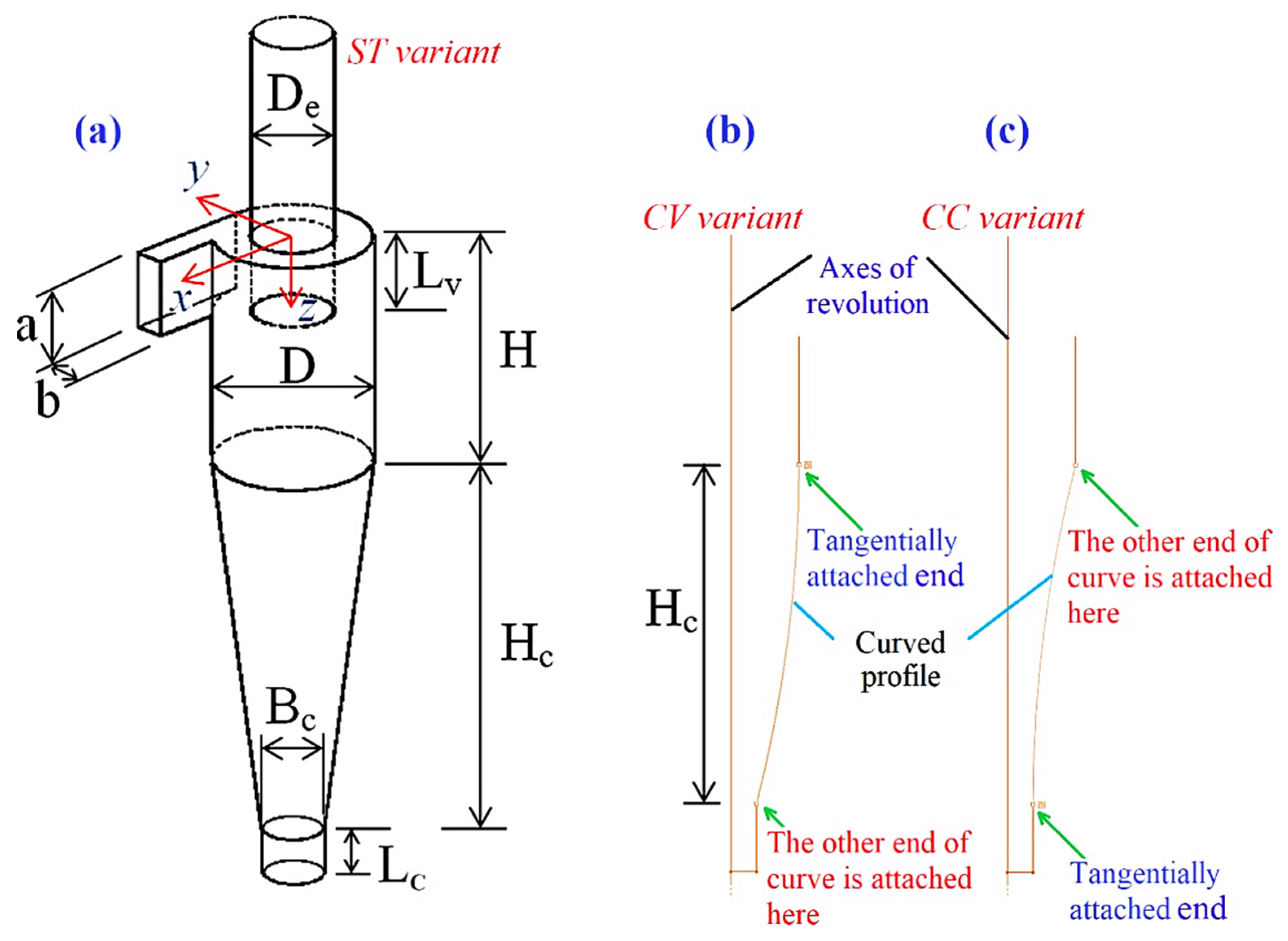
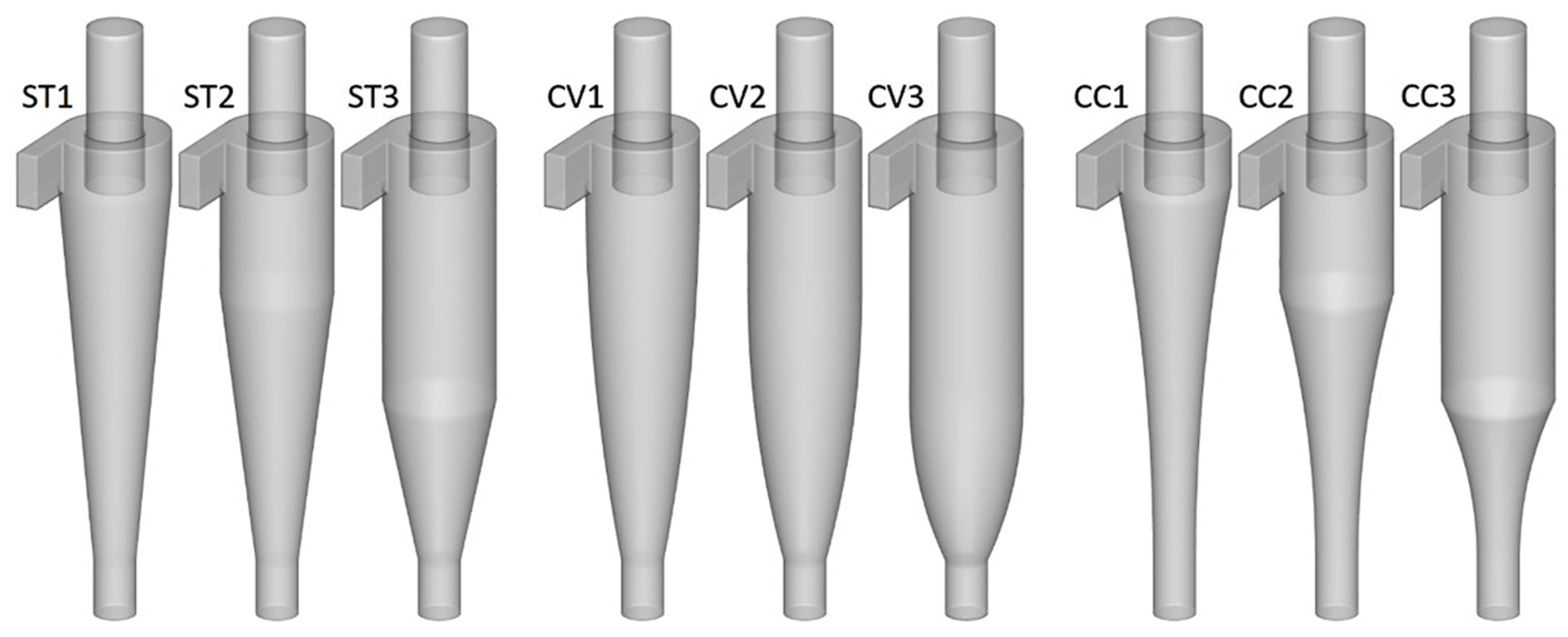
2.3. Details of the Analyzed Geometric Variants and the Adopted Assumptions of CFD Study

The performance of all the cyclone geometries considered in the present work is analysed using numerical simulations. The governing (differential) equations, which are in conservation form, are first integrated over each control volume. Next, these equations are converted into a set of linear algebraic equations, which are further solved iteratively with user-defined solver tolerance (residuals) and under-relaxation factors. Since there are no moving bodies or boundaries in the present case, the Eulerian grids are generated. However, since the secondary (particulate) phase is tracked throughout the flow field, this demands implementing the Lagrangian approach. Hence, collectively, the approach is termed the Euler-Lagrangian approach [40].

Since cyclonic flows constitute high streamlined curvatures with rapid changes in strain, and steep pressure gradients—which makes it highly anisotropic—a one equation model (viz. Spallart-Allmaras), and two-equation models (such as k-ε and k-ω closures) are not suitable here due to isotropic treatment to the turbulence. Hence, a more advanced (a seven equation) closure model to RANS viz. Reynolds stress model (RSM) is preferred, which solves transport equations for the Reynolds stresses together with an equation for the dissipation rate. RSM is capable to account for the anisotropy associated with the swirling flows [9,13,36,40].

2.3.1. Details of the Cyclone Models

The Stairmand high-efficiency cyclone model [46] is used as a baseline model to evaluate the performance of the proposed cyclone design. The cyclone Stairmand is a cylinder-on-cone structure to which the inlet of the two-phase mixture (solid-fluid) is tangentially attached at the top. The geometry of this separator includes the following sections: two-phase mixture inlet (defined by height a and width b); vortex finder diameter (D_e) and length (L_v); the diameter of the lower conical section (B_c); the height of the cylindrical section (H), the height of the conical section (H_c), the dipleg height (L_c), and cyclone diameter (D), as shown in Figure 1a; the dimensions are given in

Table 1. Dimensions of the cyclone models.

Cyclone Variants	Cyclones Models	Symbol	Dimensionless Ratio (Dimension)/D
		De	0.5
		a	0.5
		b	0.2
		Lv	0.5
		Lc	0.5
		Bc	0.375
ST	ST1	H	0.5
	ST2 *		1.5
	ST3		2.5
CV	CV1		0.5
	CV2		1.5
	CV3		2.5
CC	CC1		0.5
	CC2		1.5
	CC3		2.5
ST	ST1	Hc	3.5
	ST2		2.5
	ST3		1.5
CV	CV1		3.5
	CV2		2.5
	CV3		1.5
CC	CC1		3.5
	CC2		2.5
	CC3		1.5

* Standard (Stairmand high efficiency) cyclone model with D = 0.205 m.

.

Apart from the straight walls of the conical section (referred to as the ST (straight) variant), we also consider curved conical walls. For this, the two proposed curved geometries include a convex profile (referred to as the CV variant, cf. Figure 1b), and a concave profile (referred to as the CC variant, cf. Figure 1c)—the profile description is based on the observations external to the cyclone. The convex profile, as shown in Figure 1b, consists of a parabolic curve attached tangentially to the vertical line of the cylinder at the top, while the other end is attached to a short downcomer tube. On the other hand, in the concave profile (cf. Figure 1c), one end is attached tangentially to the downcomer tube, whereas the other end is attached to the cylindrical section at the top. After completion of (2-D) geometry on the y plane, the cyclone model was generated by revolving the profile about the (z-) axis of revolution. As a final step, a rectangular duct was attached to all models near the cyclone roof.

In addition to the above, we further explore the impact of different heights of the cylindrical section on the cyclone performance—the height of the cylinder is changed while maintaining a constant total cyclone height (H + H_c). The reason for not permitting any change to the total height is to optimize the design for a compact size. Such an approach was considered earlier by authors [15,39,40]. The details of all the cyclone geometries are given in Table 1, and the final geometries of all the models are represented in Figure 2.

To summarize, in the present study, we categorize the cyclone variants based on the profile of the conical wall viz. a straight profile (ST variant), convex profile (CV variant) and concave profile (CC variant). The different heights of the cylindrical section in each variant are then further categorized as the cyclone models that contain a numeric character after the variant description (cf. Figure 2).

2.3.2. Mesh Generation and Solver Settings

Since there are no moving bodies or boundaries in the present case, the Eulerian grids are generated using ICEM CFD; in this, the block-structured mesh was created that conforms to the curved boundaries. The generated hexahedral mesh is non-orthogonal, and the cell faces are well aligned to the direction of the fluid flow—this helps to reduce numerical diffusion. Three levels of the grid are considered viz. 214K, 386K and 568K, referred to as level 1, level 2, and level 3 mesh, respectively, and evaluated for grid dependence. Details of the surface mesh (of level 2) for the cyclone models ST2, CV2, and CC2 are illustrated in Figure 3. For all the cases, and all grid resolutions, the maximum aspect ratio was 32, and the mean skewness was 0.88 (near the central brick in the core region of the cyclone). At different grid resolutions, the velocity profiles were found to be nearly the same with no remarkable difference. The maximum difference in pressure drop was found to be less than 3.8%, and for cut-off particle size, the maximum difference was 3%.

In the present study—assuming a low volume fraction of solid particles loading (less than 10% by volume)—we consider one-way coupling. This has been considered in numerous studies (e.g., [8,9,10,12,17,20]) without any loss in generality. The transient simulations were initialized with reference to the inlet velocity and zero gauge pressure at the inlet.

For pressure and velocity coupling, we use the SIMPLEC algorithm. For pressure discretization, we use the PRESTO! interpolation scheme. The momentum equations are discretized using the QUICK scheme. For turbulent kinetic energy and dissipation rate, the second-order upwind scheme is used. For a stable solution, the first-order upwind scheme is applied to Reynolds stresses. The solver tolerance is set to 1 × 10⁻⁵ for all the conservation equations. A time step size of 0.0001 s is used for the considered variants. To account for the near-wall effects, we use the standard wall function. Such numerical settings were also used by [16,47,48,49,50].

For the solid particles, 1,000,000 integral steps are used to keep track of the particle trajectories. A length scale of 0.005 m has been opted. To consider the effect of turbulence on solid particles in the flow field, the discrete random walk model has been applied. The characteristic lifetime of an eddy is accounted for using the random eddy lifetime model with a trapezoidal discretization scheme [16,17,51].

2.3.3. Materials and Boundary Conditions

For the continuous phase, air with a density of 1200 kg/m³ and viscosity equal to 2 × 10⁻⁵ kg/m^−s has been used. The velocity inlet boundary condition ($\overline{\mathit{U}}=-U_{in}\widehat{n}$.) [52,53] with turbulent intensity ($I=u^{\prime }/U_{in}$; u′ as the root mean square of the velocity) set to 5% is used at the inlet and a uniform velocity profile is applied. At the cyclone outlet, the pressure outlet boundary condition (with zero-gauge pressure) is applied. All other walls of the cyclone separator were assigned a no-slip boundary condition ($\mathit{u}·\widehat{n}=0$. ) [52,53]. Three different inlet velocities viz. U_in =10, 15, and 20 m/s are considered in the present study to analyse the performance of all cyclone models.

The solid phase was talcum powder ρ_p = 2700 kg/m³). For solid particles, the uniformly sized particles are considered with eight different sizes ranging from 0.4 to 8.0 µm—these particles are introduced from the inlet in the direction normal to the inlet face. The solids touching the bottom plate are considered to be collected by the cyclone; hence, the trap boundary condition is applied there. The escape boundary condition is applied at the outlet plane, and the solid particles that pass through this plane are considered uncollected. Assuming a nearly perfect elastic collision between the solid particles and cyclone walls, the coefficient of restitution in tangential as well as wall-normal direction is taken as unity.

Two criteria were chosen for convergence viz. the residuals and the monitored flow variables. Regarding the former, the simulation was considered converged when the flow residuals fall below the targeted value of 10⁻⁵, and for the latter, the tangential velocity was monitored at several locations in the flow domain and it was ensured that the monitored value becomes (quasi-) steady with time.

2.4. Validation

For validation, we use the experimental data of Slack et al. [54] in which the Stairmand [46] with main body diameter, D = 0.205 m was used. The geometrical details have already been presented in Table 1, with the ST2 variant resembling the one used in [54]. At the inlet, a uniform velocity profile has been prescribed amounting to Re = 2.58 × 10⁵, as used in the experiment.

Figure 4 elucidates the comparison of the present numerical simulations against the experimental data by [54]. The first column represents radial profiles of mean axial velocity, and the second column shows the mean tangential velocity at axial locations Z/D = 0.811, 1.104, 2.128, and 3.006 (from top to bottom), respectively. At all the axial locations, the mean axial velocity agrees well both qualitatively and quantitatively—the local dip near the cyclone axis and the local maxima on either side of the axis are very well captured. The tangential velocity is also in good agreement with the reference data. Although a mild difference is observed in the upper part of the cyclone, in the conical section the local peaks match very well. Since the cyclonic flows are known to constitute a high level of anisotropy followed by the Rankine vortex, the numerical results presented here may be considered to fit well with the measured data. Two levels of mesh consisting of nearly 385K and 624K hexahedra were tested. Since no appreciable difference was noticed, the results of level 2 have been presented in Figure 4.

A mild difference is observed in the axial velocity profiles and tangential velocity profiles when compared to the reference data due to a high level of anisotropy and complex flow phenomenon. Such differences are also reported in several studies even with the advanced closure LES; for instance [1,5,6,7,8,9,10,12,13,14,15,16,17,18,19,20].

3. Results and Discussion

In this section, we present the performance parameters of each cyclone model, followed by a detailed analysis of the mean flow field. Contour plots are represented over the Y = 0 plane, whereas the mean radial profiles are calculated at different axial locations. Finally, the pressure drop, cut-off particle size and overall separation efficiency in all models—also at different U_in—are computed and compared.

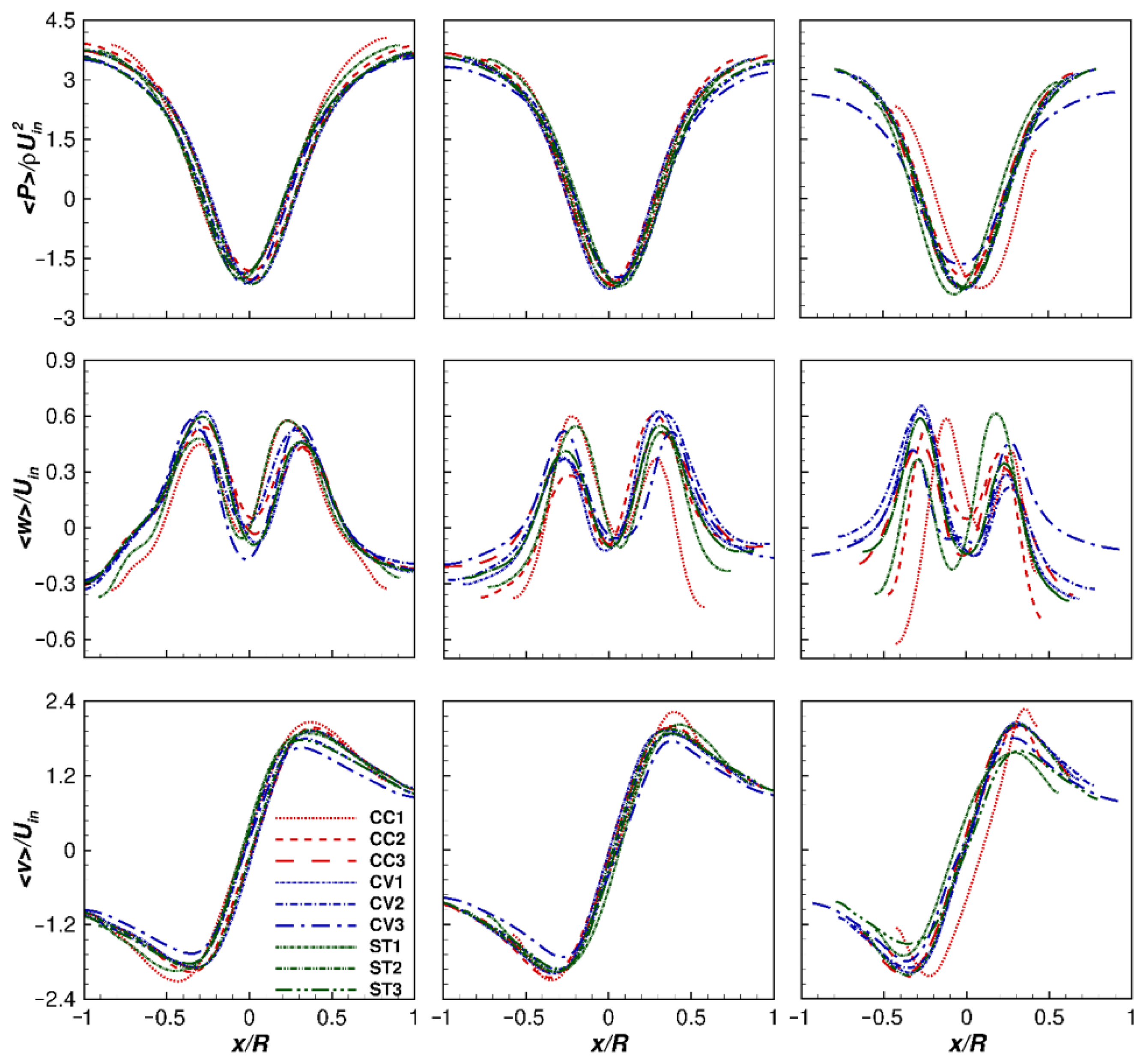
3.1. Continuous Phase

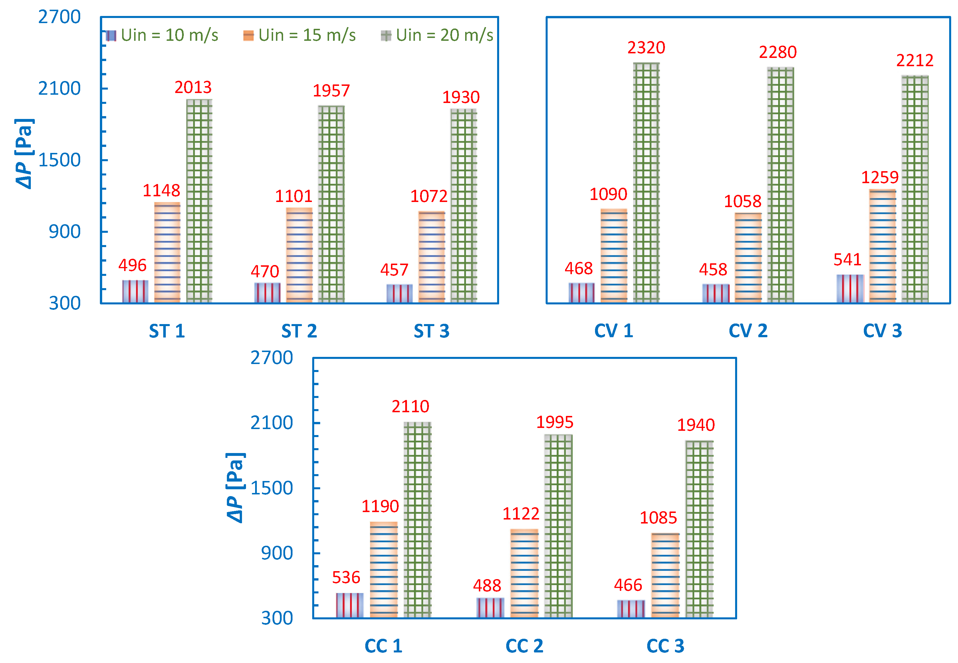
The first row in Figure 5 shows the contour plot of mean static pressure over the Y = 0 plane (normalized with the density times the square of the inlet velocity magnitude). The pressure distribution is nearly the same in all the models. In the core region, a negative pressure zone is observed—this means that the pressure there falls below the atmospheric pressure (the gauge pressure values have been used). The static pressure near the (outer) solid walls in the separation region is the highest, and this value reduces significantly when approaching the cyclone centre. The first row in Figure 6 illustrates the radial profiles of mean static pressure at z/D = 1.0, 2.0, and 3.0, from left to right, respectively. When moving along a radial direction, the pressure variations are smaller in the outer vortex region, and significant in the core region—large pressure gradients exist in the latter zone. The wall static pressure is the largest in the CC variant and lowest in the CV variant, with intermediate values in the ST variant. Furthermore, in each variant, the pressure values reduce from model 1 to 3. The wall static pressure reduces largely near the cyclone bottom, particularly in the CC variant, and in model ST1 (the same can be observed at the lowest axial location (z/D = 3.0)). It is also interesting to notice that the wall pressure is highly asymmetric in cyclone model CC1. This is due to a significant bending of the vortex core and a reduction in the cross-sectional area down the cyclone. The cyclone models having larger wall pressure values are expected to yield larger pressure drops.

The second row in Figure 5 presents the contour plots of mean axial velocity (normalized with the inlet velocity). It becomes apparent that this velocity component has two regions viz. the outer vortex swirling in the downward direction and the inner vortex directed upward—the former takes up the negative axial velocity values, whereas the latter is positive. Seemingly, the axial velocity pattern is nearly similar in all variants, except that the zone confined to the upward movement of the fluid is narrower in the CC variant and wider in the CV variant. The second row in Figure 6 represents the mean radial profiles at different locations. The downward directed flow has maximum magnitude near the outer walls, and it reduces when moving radially inwards till it becomes zero at a radial location. Thereafter, the axial velocity takes positive values in the rest of the region, indicating a movement in the upward direction. Furthermore, the axial velocity exhibits a local dip near the cyclone axis that takes up a small negative value at the geometric axis, indicating a narrow backflow region. The variations are more in the outer region than in the core region—at z/D = 1.0, small changes persist, and this difference increases with z/D values. At z/D = 2.0, larger variations can be noticed near the walls and become maximum at z/D = 3.0. In the CC variant, the axial velocity near the walls is much higher, particularly in the lower sections of the cyclone. The variations are significantly high with changes in the length of the cylindrical section in each model, particularly in the cone region. Also Demir et al. [55] noted a significant influence of the length of the cylindrical section on the values of the velocity components.

The third row in Figure 5 elucidates the contour plots of mean tangential velocity in all models. This is the most important component of velocity as it directly controls the strength of the centrifugal force field generated in cyclones, which in turn influences the collection efficiency and pressure drop. The tangential velocity distribution is nearly the same in all cyclone models, and it is seemingly zero near the geometric axis; thereafter it takes up the maximum value in the core region. More detailed information can be found in the last line of Figure 6 which shows the radial profiles of mean tangential velocity at different axial locations. It becomes apparent that in the core region, the tangential velocity varies linearly—it is zero near the rotational axis of the inner vortex and increases linearly in the core region till it reaches the maximum value. Thereafter, the tangential velocity magnitude decreases rapidly in a nonlinear manner and reduces significantly near the outer walls. The peak value of tangential velocity is maximum in the CC variant and minimum in the CV variant. Furthermore, in each variant, the velocity decreases from model 1 to 3. Interestingly, the outer vortex region is very narrow in the CC variant, particularly in the lower part of the cyclone where a large asymmetric distribution is a sough. The region confined to the inner vortex is hardly affected. Since tangential velocity governs the centrifugal flow field, the cyclone models experiencing larger tangential magnitude are likely to undergo larger pressure drops.

3.2. Pressure Drop

In the present study, the pressure drop is taken as the difference in the mean total pressure values at the inlet surface and outlet surface. This factor is proportional to the energy that a cyclone would require to operate. Higher pressure drop signifies large irreversible losses, and so, higher energy is required to make the fluid flow through the cyclone volume, and vice-versa. Since these devices operate continuously for a longer time in several applications, the proposed design must ensure low-pressure losses.

Figure 7 presents the pressure drop values in the cyclone variants at different inlet velocities, categorized as variants. With an increase in the inlet velocity, pressure drop increases significantly. For a given cylinder length, in comparison with the ST variant, the pressure drop is lowest in models 1 and 2 of the CV variant, whereas in the CC variant all the models elucidate an increased pressure drop. At U_in = 10 m/s and 15 m/s, models 1 and 2 in the CV variant shows lower pressure losses than in the ST variant. Interestingly, for all U_in, the pressure drop value in model 3 of the CV variant is greater than in the ST variant (as an exception, a similar observation also holds for the CV1 model at U_in = 20 m/s). This could be due to the larger cross-sectional area just above the downcomer tube in the CV variant than in ST and CC variants—the area is the largest in model 3. Due to this, the flow experiences significant contraction over a small height (above the top connecting surface of the downcomer tube) that complicates the flow, particularly at higher inlet velocities. In contrast to the CV variant, the results are more consistent in the CC variant when compared with the ST variant. Here, at a given U_in and cylinder length, the pressure drop is larger in all the models in the CV variant than in the CC variant. Another important observation is that the pressure drop also reduces with an increase in the length of the cylindrical section at a given U_in. A similar trend was found by Demir et al. [55] in their studies on effects of cylindrical and conical heights on pressure and velocity fields.

Table 2. Pressure drop at different inlet velocities.

Cyclone Variants	Cyclone Models	% Change in Pressure Drop *
		Uin = 10 m/s	Uin = 15 m/s	Uin = 20 m/s
ST	ST1	5.53	4.27	2.86
	ST2	–	–	–
	ST3	−2.77	−2.63	−1.38
CV	CV1	−0.425	−1.00	18.55
	CV2	−2.55	−3.91	16.51
	CV3	15.11	14.35	22.12
CC	CC1	14.04	8.08	7.82
	CC2	3.83	1.91	1.94
	CC3	−0.85	−1.45	−0.87

* % Change w.r.t. the standard cyclone model ST2.

elucidates complete information on (percent change in) pressure drop with respect to the base variant model ST2, at different U_in, in all models.

3.3. Analysis of the Separation Efficiency

The main purpose of utilizing a cyclone is to separate the particles from gas, and in this regard, the separation capability of a cyclone is defined in two ways. First, the cut-off particle size (designated as x₅₀)—defined as the particle size that corresponds to 50% separation efficiency on the grade efficiency curve (GEC). Second, the overall separation efficiency is calculated as the ratio of the number of particles separated by the cyclone separator to the number of particles entering the cyclone.

Figure 8 represents the GEC of all variants at U_in = 10 m/s. The change in dimensions and shape of individual sections of the cyclone separator did not significantly change the profile of GEC curves. Similar observations were made by Shastri et al. [39] and Xiang et al. [37]. For all cylinder lengths in each variant, the variations in the GECs are from mild to moderate—CC variants are more sensitive to the cylinder height than the ST variant, whereas in the CV variant the variations are very mild. Complete information on the cut-off size for all U_in is presented in Figure 9. Two important observations here are: with an increase in cylinder length, x₅₀ increases mildly at all U_in, whereas with an increase in U_in, the cut-off size reduces significantly in all variants. For short cylinder height and lower U_in, the CC variant outperforms the ST as well as CV variants, whereas, at higher U_in, the x₅₀ values in the ST variant are greater than other variants by a very small margin.

Figure 10 illustrates the overall separation efficiency in all variants at different U_in. With an increase in U_in, the overall separation efficiency in each variant increases significantly, whereas the increase in the cylinder height mildly reduces the collection efficiency at a given U_in. The efficiency of different models in the CC variant is slightly better than the standard ST variant, and in the case of CV, the efficiency is the lowest.

Table 3. Percent change in overall separation efficiency and cut-off diameter at different U_in.

Cyclone Variants	Cyclone Models	% Change in Overall Separation Efficiency *			% Change in Cut-Off Diameter *
		Uin = 10 m/s	Uin = 15 m/s	Uin = 20 m/s	Uin = 10 m/s	Uin = 15 m/s	Uin = 20 m/s
ST	ST1	0.73	2.36	2.45	−2.16	−2.95	−2.14
	ST2	–	–	–	–	–	–
	ST3	−2.37	−2.17	−2.66	3.30	1.91	1.77
CV	CV1	−0.31	5.19	−1.78	0.36	−2.31	3.35
	CV2	−1.69	3.16	−1.74	1.26	4.55	8.93
	CV3	1.55	6.77	−0.24	1.98	6.54	13.67
CC	CC1	0.89	5.98	4.13	−7.02	−4.47	1.30
	CC2	−1.25	3.40	1.10	−1.74	0.56	5.21
	CC3	−0.52	3.60	−3.55	1.92	6.38	10.88

* % Change w.r.t. the standard cyclone model ST2.

provides complete information on (percent change in) overall separation efficiency and cut-off size with respect to the base variant ST2, at different U_in, in all variants.

4. Conclusions

In the present study, unsteady simulations were performed using RSM as a closure model to RANS. The airflow was simulated over the stationary grids, whereas the solid particles were tracked using the Lagrangian approach. Hence, we made use of the Eulerian-Lagrangian approach to model the cyclonic flow field. Nine cyclone models were simulated at three different inlet velocities viz. U_in = 10 m/s, 15 m/s, and 20 m/s—thus, a total of twenty-seven cases were simulated. We considered three cyclone variants viz. a straight wall of the conical section as in the conventional cyclone design (referred to as ST variant), a curved wall with convex profile (referred to as CV variant), and a curved wall with concave profile (referred to as CC variant)—the convex and concave terminology was adopted with reference to an observer outside the cyclone structure. Furthermore, three different lengths of the cylindrical section were considered in all the three cyclone variants keeping the total cyclone length a constant.

Based on the analysis of the obtained results, the following conclusions were defined:

• With the increase in inlet velocity:
  • Pressure drop increased significantly in all cyclone variants.
  • Cut-off particle size reduced tremendously.
  • Collection efficiency increased by a large amount.
• With an increase in the length of the cylindrical section:
  • Pressure drop was reduced in all the cyclone variants.
  • Cut-off particle size increased mildly.
  • Collection efficiency reduced by a marginal amount.
• With wall profile:
  • Pressure drop was the lowest in models 1 and 2 of the CV, particularly at U_in = 10 m/s, and 15 m/s. At U_in = 20 m/s, pressure drop was the largest in CV variants, and at U_in = 10 m/s, and 15 m/s, as compared with the ST variant, the variations were moderate.
  • Cut-off particle size showed a mild variation at a given U_in. The cut-off size was largest in CV variants, whereas this size was comparable in ST and CC variants.
  • Collection efficiency increased by a marginal amount in the CC variant and was minimum in the CV variant.

References

1. Brar, L.S.; Derksen, J.J. Revealing the details of vortex core precession in cyclones by means of large-eddy simulation. Chem. Eng. Res. Des. 2020, 159, 339–352. [Google Scholar] [CrossRef]
2. Faulkner, W.B.; Shaw, B.W. Efficiency and pressure drop of cyclones across a range of inlet velocities. Appl. Eng. Agric. 2006, 22, 155–161. [Google Scholar] [CrossRef] [Green Version]
3. Safikhani, H.; Akhavan-Behabadi, M.A.; Shams, M.; Rahimyan, M.H. Numerical simulation of flow field in three types of standard cyclone separators. Adv. Powder Technol. 2010, 21, 435–442. [Google Scholar] [CrossRef]
4. Hoffman, A.C.; Stein, L.E. Gas Cyclones and Swirl Tubes: Principles, Design and Operation; Springer: Berlin/Heidelberg, Germany, 2008. [Google Scholar] [CrossRef]
5. Brar, L.S.; Sharma, R.P.; Dwivedi, R. Effect of vortex finder diameter on flow field and collection efficiency of cyclone separators. Part. Sci. Technol. 2014, 33, 34–40. [Google Scholar] [CrossRef]
6. Wasilewski, M.; Brar, L.S. Optimization of the geometry of cyclone separators used in clinker burning process: A case study. Powder Technol. 2017, 313, 293–302. [Google Scholar] [CrossRef]
7. Wasilewski, M.; Brar, L.S.; Ligus, G. Experimental and numerical investigation on the performance of square cyclones with different vortex finder configurations. Sep. Purif. Technol. 2020, 239, 1–20. [Google Scholar] [CrossRef]
8. Elsayed, K.; Lacor, C. The effect of cyclone vortex finder dimensions on the flow pattern and performance using LES. Comput. Fluids 2013, 71, 224–239. [Google Scholar] [CrossRef]
9. Parvaz, F.; Hosseini, S.H.; Ahmadi, G.; Elsayed, K. Impacts of the vortex finder eccentricity on the flow pattern and performance of a gas cyclone. Sep. Purif. Technol. 2017, 187, 1–13. [Google Scholar] [CrossRef]
10. Brar, L.S.; Elsayed, K. Analysis and optimization of cyclone separators with eccentric vortex finders using large eddy simulation and artificial neural network. Sep. Purif. Technol. 2018, 207, 269–283. [Google Scholar] [CrossRef]
11. Pei, B.; Yang, L.; Dong, K.; Jiang, Y.; Du, X.; Wang, B. The effect of cross-shaped vortex finder on the performance of cyclone separator. Powder Technol. 2017, 313, 135–144. [Google Scholar] [CrossRef]
12. Misiulia, D.; Antonyuk, S.; Andersson, A.G.; Lundström, T.S. Effects of deswirler position and its centre body shape as well as vortex finder extension downstream on cyclone performance. Powder Technol. 2018, 336, 45–56. [Google Scholar] [CrossRef]
13. Kumar, V.; Jha, K. Multi-objective shape optimization of vortex finders in cyclone separators using response surface methodology and genetic algorithms. Sep. Purif. Technol. 2019, 215, 25–31. [Google Scholar] [CrossRef]
14. Brar, L.S.; Sharma, R.P. Effect of varying diameter on the performance of industrial scale gas cyclone dust separators. Mater. Today Proc. 2015, 4, 3230–3237. [Google Scholar] [CrossRef]
15. Brar, L.S. Application of response surface methodology to optimize the performance of cyclone separator using mathematical models and CFD simulations. Mater. Today Proc. 2018, 5, 20426–20436. [Google Scholar] [CrossRef]
16. Brar, L.S.; Sharma, R.P.; Elsayed, K. The effect of the cyclone length on the performance of Stairmand high-efficiency cyclone. Powder Technol. 2015, 286, 668–677. [Google Scholar] [CrossRef]
17. Elsayed, K.; Lacor, C. The effect of cyclone inlet dimensions on the flow pattern and performance. Appl. Math. Model. 2011, 35, 1952–1968. [Google Scholar] [CrossRef] [Green Version]
18. Wasilewski, M.; Brar, L.S. Effect of the inlet duct angle on the performance of cyclone separators. Sep. Purif. Technol. 2019, 213, 19–33. [Google Scholar] [CrossRef]
19. Brar, L.S.; Elsayed, K. Analysis and optimization of multi-inlet gas cyclones using large eddy simulation and artificial neural network. Powder Technol. 2017, 311, 465–483. [Google Scholar] [CrossRef]
20. Misiulia, D.; Andersson, A.G.; Lundström, T.S. Effects of the inlet angle on the collection efficiency of a cyclone with helical-roof inlet. Powder Technol. 2017, 305, 48–55. [Google Scholar] [CrossRef]
21. Piemjaiswang, R.; Ratanathammapan, K.; Kunchonthara, P.; Piumsomboon, P.; Chalermsinsuwan, B. CFD study of cyclone performance: Effect of inlet section angle and particle size distribution. J. Teknol. 2016, 78, 83–89. [Google Scholar] [CrossRef] [Green Version]
22. Yao, Y.; Huang, W.; Wu, Y.; Zhang, Y.; Zhang, M.; Yang, H.; Lyu, J. Effects of the inlet duct length on the flow field and performance of a cyclone separator with a contracted inlet duct. Powder Technol. 2021, 393, 12–22. [Google Scholar] [CrossRef]
23. Wang, Z.; Sun, G.; Jiao, Y. Experimental study of large-scale single and double inlet cyclone separators with two types of vortex finder. Chem. Eng. Process.-Process Intensif. 2020, 158, 108188. [Google Scholar] [CrossRef]
24. Qiang, L.; Qinggong, W.; Weiwei, X.; Zilin, Z.; Konghao, Z. Experimental and computational analysis of a cyclone separator with a novel vortex finder. Powder Technol. 2020, 360, 398–410. [Google Scholar] [CrossRef]
25. Le, D.K.; Yoon, J.Y. Numerical investigation on the performance and flow pattern of two novel innovative designs of four-inlet cyclone separator. Chem. Eng. Process.-Process Intensif. 2020, 150, 107867. [Google Scholar] [CrossRef]
26. Noh, S.Y.; Heo, J.E.; Woo, S.H.; Kim, S.J.; Ock, M.H.; Kim, Y.J.; Yook, S.J. Performance improvement of a cyclone separator using multiple subsidiary cyclones. Powder Technol. 2018, 338, 145–152. [Google Scholar] [CrossRef]
27. Wasilewski, M.; Brar, L.S.; Ligus, G. Effect of the central rod dimensions on the performance of cyclone separators-optimization study. Sep. Purif. Technol. 2021, 274, 119020. [Google Scholar] [CrossRef]
28. Parvaz, F.; Hosseini, S.H.; Elsayed, K.; Ahmadi, G. Influence of the dipleg shape on the performance of gas cyclones. Sep. Purif. Technol. 2020, 233, 116000. [Google Scholar] [CrossRef]
29. Xu, M.; Yang, L.; Sun, X.; Wang, J.; Gong, L. Numerical analysis of flow resistance reduction methods in cyclone separator. J. Taiwan Inst. Chem. Eng. 2019, 96, 419–430. [Google Scholar] [CrossRef]
30. Qiang, L.; Jianjun, W.; Weiwei, X.; Meng, Z. Investigation on separation performance and structural optimization of a two-stage series cyclone using CPFD and RSM. Adv. Powder Technol. 2020, 31, 3706–3714. [Google Scholar] [CrossRef]
31. Galletti, C.; Rum, A.; Turchi, V.; Nicolella, C. Numerical analysis of flow field and particle motion in a dynamic cyclonic selector. Adv. Powder Technol. 2020, 31, 1264–1273. [Google Scholar] [CrossRef]
32. Sun, Z.; Liang, L.; Liu, Q.; Yu, X. Effect of the particle injection position on the performance of a cyclonic gas solids classifier. Adv. Powder Technol. 2020, 31, 227–233. [Google Scholar] [CrossRef]
33. Fu, S.; Zhou, F.; Sun, G.; Yuan, H.; Zhu, J. Performance evaluation of industrial large-scale cyclone separator with novel vortex finder. Adv. Powder Technol. 2021, 32, 931–939. [Google Scholar] [CrossRef]
34. Mofarrah, M.; Hojjat, Y.; Mashayekh, S.; Liu, Z.; Yan, K. Introduction and simulation of a small electro cyclone for collecting indoor pollen particles. Adv. Powder Technol. 2021, 33, 103384. [Google Scholar] [CrossRef]
35. An, I.H.; Lee, C.H.; Lim, J.H.; Lee, H.Y.; Yook, S.J. Development of a miniature cyclone separator operating at low Reynolds numbers as a pre-separator for portable black carbon monitors. Adv. Powder Technol. 2021, 32, 4779–4787. [Google Scholar] [CrossRef]
36. Gimbun, J.; Chuah, T.G.; Choong, T.S.Y.; Fakhru’l-Razi, A. Prediction of the effects of cone tip diameter on the cyclone performance. Aerosol Sci. 2005, 36, 1056–1065. [Google Scholar] [CrossRef]
37. Xiang, R.; Park, S.H.; Lee, K.W. Effects of cone dimension on cyclone performance. J. Aerosol Sci. 2001, 32, 549–561. [Google Scholar] [CrossRef]
38. Stern, A.; Caplan, K.; Bush, P. Cyclone Dust Collectors; American Petroleum Institute: New York, NY, USA, 1955. [Google Scholar]
39. Shastri, R.; Brar, L.S. Numerical investigations of the flow-field inside cyclone separators with different cylinder-to-cone ratios using large-eddy simulation. Sep. Purif. Technol. 2020, 249, 1–17. [Google Scholar] [CrossRef]
40. Shastri, R.; Sharma, R.P.; Brar, L.S. Numerical investigations of cyclone separators with different cylinder-to-cone ratios. Part. Sci. Technol. 2021, 40, 337–345. [Google Scholar] [CrossRef]
41. Ghodrat, M.; Kuang, S.B.; Yu, A.B.; Vince, A.; Barnett, G.D.; Barnett, P.J. Numerical analysis of hydrocyclones with different conical section designs. Miner. Eng. 2014, 62, 74–84. [Google Scholar] [CrossRef]
42. Wilcox, D.C. Turbulence Modeling for CFD; DCW Industries, Inc.: La Cañada Flintridge, CA, USA, 1994. [Google Scholar]
43. Fluent Theory Guide; Fluent Inc.: Canonsburg, PA, USA, 2016.
44. Morsi, A.J.; Alexander, S.A. An Investigation of Particle Trajectories in Two-Phase Flow System. J. Fluid Mech. 1972, 55, 193–208. [Google Scholar] [CrossRef]
45. Shukla, S.K.; Shukla, P.; Ghosh, P. Evaluation of Numerical Schemes for Dispersed Phase Modeling of Cyclone Separators. Eng. Appl. Comp. F Mech. 2010, 5, 235–246. [Google Scholar] [CrossRef] [Green Version]
46. Stairmand, C.J. The design and performance of cyclone separators. Ind. Eng. Chem. 1951, 29, 356–383. [Google Scholar]
47. Wasilewski, M. Analysis of the effects of temperature and the share of solid and gas phases on the process of separation in a cyclone suspension preheater. Sep. Purif. Technol. 2016, 168, 114–123. [Google Scholar] [CrossRef]
48. Wasilewski, M. Analysis of the effect of counter-cone location on cyclone separator efficiency. Sep. Purif. Technol. 2017, 179, 236–247. [Google Scholar] [CrossRef]
49. Wasilewski, M.; Brar, L.S. Investigations of the flow field inside a square cyclone separator using DPIV and CFD. E3S Web Conf. 2019, 100, 1–8. [Google Scholar] [CrossRef]
50. Venkatesh, S.; Kumar, R.S.; Sivapirakasam, S.P.; Sakthivel, M.; Venkatesh, D.; Arafath, S.Y. Multi-objective optimization, experimental and CFD approach for performance analysis in a square cyclone separator. Powder Technol. 2020, 371, 115–129. [Google Scholar] [CrossRef]
51. Wasilewski, M.; Duda, J. Multicriteria optimisation of first-stage cyclones in the clinker burning system by means of numerical modelling and experimental research. Powder Technol. 2016, 289, 143–158. [Google Scholar] [CrossRef]
52. Stachnik, M.; Jakubowski, M. Multiphase model of flow and separation phases in a whirlpool: Advanced simulation and phenomena visualization approach. J. Food Eng. 2020, 274, 109846. [Google Scholar] [CrossRef]
53. Jakubowski, M.; Sterczyska, M.; Matysko, R.; Poreda, A. Simulation and experimental research on the flow inside a whirlpool separator. J. Food Eng. 2014, 133, 9–15. [Google Scholar] [CrossRef]
54. Slack, M.D.; Prasad, R.O.; Bakker, A.; Boysan, F.M. Advances in Cyclone Modelling Using Unstructured Grids. Chem. Eng. Res. Des. 2000, 78, 1098–1104. [Google Scholar] [CrossRef]
55. Demir, S.; Karadeniz, A.; Aksel, M. Effects of cylindrical and conical heights on pressure and velocity fields in cyclones. Powder Technol. 2016, 295, 209–217. [Google Scholar] [CrossRef]
Figure 1. Geometrical details of the Stairmand high-efficiency cyclone model (D = 0.205 m) with (a) straight walls of the conical section (referred to as the ST), (b) convex profile (referred to as the CV variant), and (c) concave profile (referred to as the CC variant).
Applsci 12 04904 g001
Figure 2. Structural representation of all the cyclone models of ST variant, CV variant and CC variant (from left to right), respectively.
Applsci 12 04904 g002
Figure 3. Sample mesh regions for all cyclone models ST1, CV1, and CC1. Three levels of the grid are considered viz. 214K, 386K and 568K (from left to right), respectively.
Applsci 12 04904 g003
Figure 4. Comparative analysis of CFD results with experimental data [54]: (a) the first column—mean axial velocity; the second column—mean tangential velocity, and (b) from top to bottom: radial profiles at axial locations Z/D = 0.811, 1.104, 2.128, and 3.006 (D = 2R = 0.205 m is the barrel diameter) from the cyclone roof, respectively.
Applsci 12 04904 g004
Figure 5. Contour plots on Y/D = 0 plane at Uin = 10 m/s. From left to right: different cyclone models. From top to bottom: mean static pressure, mean axial velocity, and mean tangential velocity.
Applsci 12 04904 g005
Figure 6. From left to right: the radial profiles at z/D = 1.0, 2.0, and 3.0 of mean static pressure, mean axial velocity and mean tangential velocity (top to bottom), respectively, in different cyclone models.
Applsci 12 04904 g006
Figure 7. Pressure drop values in all the cyclone models of ST variant, CV variant and CC variant at inlet velocities, Uin = 10, 15 and 20 m/s.
Applsci 12 04904 g007
Figure 8. Grade efficiency curves for all cyclone models in ST variant, CV variant and CC variant at inlet velocities Uin = 10 m/s with particle sizes ranging from 0.4 to 8.0 µm.
Applsci 12 04904 g008
Figure 9. Cut-off sizes in all cyclone models of ST variant, CV variant, and CC variant at inlet velocities Uin = 10, 15 and 20 m/s.
Applsci 12 04904 g009
Figure 10. Overall separation efficiency in all the cyclone models of ST variant, CV variant and CC variant at inlet velocities Uin = 10, 15 and 20 m/s.
Applsci 12 04904 g010