Article

Accounting for Patient Engagement in Randomized Controlled Trials Evaluating Digital Cognitive Behavioral Therapies

by
Oleksandr Sverdlov
1,* and
Yevgen Ryeznik
2
1
Novartis Pharmaceuticals Corporation, East Hanover, NJ 07936, USA
2
AstraZeneca, 43183 Mölndal, Sweden
*
Author to whom correspondence should be addressed.
Appl. Sci. 2022, 12(10), 4952; https://doi.org/10.3390/app12104952
Submission received: 19 February 2022 / Revised: 2 May 2022 / Accepted: 10 May 2022 / Published: 13 May 2022
(This article belongs to the Special Issue Digital Therapeutics Applications for Chronic Disease Management)

Abstract

:
Background: Cognitive behavioral therapy (CBT) can be a useful treatment option for various mental health disorders. Modern advances in information technology and mobile communication enable delivery of state-of-the-art CBT programs via smartphones, either as stand-alone or as an adjunct treatment augmenting traditional sessions with a therapist. Experimental CBTs require careful assessment in randomized clinical trials (RCTs). Methods: We investigate some statistical issues for an RCT comparing efficacy of an experimental CBT intervention for a mental health disorder against the control. Assuming a linear model for the clinical outcome and patient engagement as an influential covariate, we investigate two common statistical approaches to inference—analysis of covariance (ANCOVA) and a two-sample t-test. We also study sample size requirements for the described experimental setting. Results: Both ANCOVA and a two-sample t-test are appropriate for the inference on treatment difference at the average observed level of engagement. However, ANCOVA produces estimates with lower variance and may be more powerful. Furthermore, unlike the t-test, ANCOVA allows one to perform treatment comparison at the levels of engagement other than the average level observed in the study. Larger sample sizes may be required to ensure experiments are sufficiently powered if one is interested in comparing treatment effects for different levels of engagement. Conclusions: ANCOVA with proper adjustment for engagement should be used for the for the described experimental setting. Uncertainty on engagement patterns should be taken into account at the study design stage.

1. Introduction

Cognitive behavioral therapy (CBT) can be useful for various mental health problems including depression, anxiety, substance use disorders, etc. Digital cognitive behavioral therapy (dCBT)—administered either as stand-alone or as an adjunct treatment augmenting traditional sessions with a human therapist—is a potentially promising way to deliver CBT by means of digital technologies such as smartphones. Potential merits of the dCBT include accessibility and cost-efficiency (e.g., real time coaching and support can be provided remotely instead of face-to-face visits), more consistent quality of treatment delivery (e.g., psychological therapy is provided by clinically validated computer programs), and personalization of treatment (e.g., the course of therapy is tailored to an individual patient’s goals, availability, and engagement) [1,2].
Fundamentally, clinical investigation of an experimental dCBT should follow a similar path to clinical trials of other therapeutic interventions [3]. The randomized controlled trial (RCT) is the most rigorous research design to obtain evidence in support of clinical efficacy of a dCBT product. However, such trials pose some unique challenges. First, many dCBTs are complex interventions with multiple ingredients that are applied based on a dynamic feedback loop to optimize the treatment for an individual patient. Second, it may be very difficult to define an optimal “dose” or “exposure” of a dCBT to attain the desired therapeutic effect [4]. Third, while engagement with dCBT is viewed as an essential component of this treatment modality [5], it is quite challenging to quantify and build reliable statistical models relating engagement with clinical efficacy. For instance, “more time using a digital therapeutic” does not necessarily translate into “better treatment effect” [6]. Fourth, high heterogeneity in the usage/engagement patterns may potentially confound treatment effects. For instance, if patients are randomized to treatments that do not meet their expectations, this may affect the patients’ motivation to engage and comply with the treatments, which, in turn, may impact the study outcomes [7].
Engagement may be strongly correlated with efficacy of an intervention. On the other hand, engagement by itself is not sufficient; for instance, study participants may enjoy using the app and provide very positive feedback, but this may not directly translate into clinical benefit. Acquiring important data on engagement and properly accounting for it in the analysis may be essential for valid statistical inference.
In this paper, we investigate some statistical issues for a 1 : 1 RCT comparing efficacy of an experimental CBT intervention for a mental health disorder versus control. For illustration purposes, we assume that participants in both experimental and control groups receive some background standard of care medication throughout the study. Participants in the experimental group (intervention condition) have sessions with a human therapist at which they learn some novel cognitive and behavioral strategies to overcome difficulties in their daily lives, and, in addition, they receive a smartphone app that augments the sessions by providing personalized tips on disease management, e.g., through serious games, educational videos, etc., that are expected to magnify therapeutic benefit. Therefore, in the experimental group the intervention has two components: novel cognitive behavioral therapy delivered during sessions with a human therapist (CBT) and a self-administered digital cognitive behavioral therapy (dCBT). Participants in the control group just have regular sessions with a therapist (without being exposed to a novel CBT) and use a sham app (without active therapeutic ingredients of a psychosocial intervention) on their smartphones.
We assume the primary endpoint Y represents some measure of clinical efficacy, e.g., change from baseline to the end of treatment period in Montgomery-Åsberg Depression Rating Scale (MADRS) [8] total score in depression. In the experimental group, participants may engage differentially with the dCBT. For simplicity, we assume that X = the percentage of successfully completed dCBT trainings at the end of the treatment period provides a meaningful quantification of individual engagement with the dCBT. While the utility of “completion rate” as a measure of engagement for digital mental health interventions has been well documented [9,10,11,12], we acknowledge that this is only one way to measure engagement. In practice, other, more elaborate metrics may be considered. However, in our opinion, a simple metric such as “completion rate” is rather informative and can be used as a starting point for developing statistical models. In other words, we assume that engagement X is measured on a scale 0 to 1, where 0 means 0% completed trainings, 0.6 means 60% completed trainings, etc. By contrast, in the control group, the sham application has no active therapeutic ingredients of a psychosocial intervention, and therefore, the engagement is a structural zero for every participant in the control group. To illustrate the latter point, consider, for example, a recent randomized, sham-controlled clinical trial of a smartphone-based application as an adjunct to the standard-of-care in schizophrenia [6]. Participants in the experimental group were exposed for a period of 12 weeks to an app that was designed as a self-management tool in schizophrenia. The users could engage with the app by prompt or on demand, and the app provided interactive, cognitive and behavior exercises that were hypothesized to improve schizophrenia symptoms. Participants in the sham group were exposed for 12 weeks to an app that was similar in appearance to the experimental app, but which did not deliver any active therapeutic content (it only sent periodic prompts to open the app, in which case a digital clock timer was displayed). The sham control arm was chosen to account for the nonspecific effects of engagement with a smartphone. Clearly, in this case the engagement defined as “exercise completion rate” can be quantified only in the experimental group, and it can be regarded as zero in the control group.
For the considered setting ( 1 : 1 RCT; primary endpoint Y is changed from the baseline in MADRS total score at the end of the treatment period; engagement X is an important covariate for subjects in the experimental group but not in the control group; no missing data in the study) we address the following research questions:
  • What is the proper approach to the statistical analysis of such a trial?
  • How do we compare treatment effects accounting for different levels of engagement?
  • How should we perform a sample size planning for such a trial given that engagement patterns are unknown upfront?
The results presented here should aid trial statisticians in developing statistical analysis plans and in facilitating important discussions with clinical investigators at the study planning stage.
The article is organized as follows. In Section 2, we describe the trial setup, assumptions for the data generating mechanism, and two approaches to data analysis following the trial—analysis of covariance (ANCOVA) and a two-sample t-test. In Section 3, we give an illustrative example of how to analyze data from such an experiment. In Section 4, we present results from a simulation study to evaluate the power of statistical tests. In Section 5, we discuss the optimization of the trial design and considerations for the sample size planning. Finally, Section 6 provides a summary and a discussion of the future work.

2. Statistical Modeling and Some Theoretical Results

We assume equal ( 1 : 1 ) RCT design for which an even number of n subjects are randomized between the experimental (E) and the control (C) conditions. Let δ i = 1 (or 0), if the i th participant is randomized to group E (or C). With equal allocation design, the group sample sizes are n E = i = 1 n δ i = n / 2 and n C = i = 1 n 1 δ i = n / 2 .
For the i th participant, we acquire data ( Y i , X i , δ i ) ( i = 1 , , n ) , where Y i is the response, δ i is the treatment assignment indicator, and X i is the measure of engagement (applicable only to the experimental group). The responses Y i , conditional on X i = x i and δ i , are assumed to satisfy the following statistical model:
Y i = δ i μ E + ( 1 δ i ) μ C + γ x i δ i + ε i , i = 1 , , n ,
where μ E and μ C are the treatment effects for group E and group C, respectively, γ is a linear regression slope, and ε i ’s are independent and identically distributed (i.i.d.) measurement errors, assumed to be normally distributed with zero mean and variance σ 2 , i.e., ε i N ( 0 , σ 2 ) .
The parameters in Equation (1) can be interpreted as follows: μ E is the effect of the novel CBT alone, i.e., this is the mean effect for a subject in the experimental group who had CBT sessions (required by the study design) and never used the dCBT (engagement level x = 0 ). On the other hand, if a subject in the experimental group had both CBT and engaged with the dCBT ( x > 0 ), then the mean response for this subject is E Y = μ E + γ x , which can be magnified or decreased compared to μ E according to the values of x and γ . For subjects in the control group, μ C is the mean effect due to the control intervention (a combination of the standard CBT and the sham app).
In the described setting, several estimands may be of interest:
(I)
The difference Δ 0 = μ E μ C , which is the contrast between the novel CBT alone and the control intervention.
(II)
The difference Δ x = ( μ E + γ x ) μ C , which is the contrast between the novel CBT + dCBT engaged at the level X = x and the control intervention.
The estimand (I) is a special case of estimand (II) with x = 0 . In practice, estimand (II) may be more relevant because it provides information on a combined effect of novel CBT + dCBT for a chosen level of x that is deemed important to the investigator. One particularly interesting case is Δ x ¯ E = ( μ E + γ x ¯ E ) μ C , which is the contrast between novel CBT + dCBT at the average level of engagement observed in the trial and the control condition.
An investigator may wish to answer to different research questions in the study, such as: (i) Is the difference Δ 0 = μ E μ C significant? (ii) Is the effect of engagement (the linear slope γ ) significant? (iii) Is the difference Δ x = ( μ E + γ x ) μ C for a pre-specified value of x significant?
The choice of the primary research question is very important because it will, among other considerations, drive the choice of the sample size for the study. The answers to questions (i)–(iii) will carry different implications for development. For instance:
  • If both Δ 0 and γ are significantly different from zero, then the novel CBT is deemed efficacious, and its effect can be magnified or decreased by the individual engagement with the dCBT.
  • If Δ 0 is significantly different from zero but γ is not, then the novel CBT is deemed efficacious but the engagement with the dCBT is not helpful for synergizing this effect.
  • If Δ x ¯ E = ( μ E + γ x ¯ E ) μ C is significantly different from zero, then a combination of the novel CBT with the dCBT engaged at the average level observed in the trial is more efficacious than the control condition.
We now present statistical approaches to address the research questions for the described problem.

2.1. Analysis of Covariance (ANCOVA)

Let θ = ( μ E , μ C , γ ) . Then, assuming model (1) is correctly specified, the ordinary least squares estimator θ ^ = ( μ ^ E , μ ^ C , γ ^ ) for θ is obtained using linear model theory [13] as
μ ^ E = Y ¯ E γ ^ x ¯ E μ ^ C = Y ¯ C γ ^ = S x y / S x x
where S x y = i = 1 n / 2 x i x ¯ E Y i Y ¯ E and S x x = i = 1 n / 2 x i x ¯ E 2 .
By Gauss–Markov theorem, θ ^ is best linear unbiased estimator of θ , i.e., θ ^ has smallest variance among all linear unbiased estimators. The variance–covariance matrix of θ is
var θ ^ = σ 2 2 n + x ¯ E 2 S x x 0 x ¯ E S x x 0 2 n 0 x ¯ E S x x 0 1 S x x .
  • Inference on Δ 0 = μ E μ C
The point estimate of Δ 0 = μ E μ C is Δ ^ 0 = μ ^ E μ ^ C , where μ ^ E and μ ^ C are from Equation (2). Note that Δ ^ 0 follows a normal distribution with mean ( μ E μ C ) and variance
var μ ^ E μ ^ C = σ 2 4 n + x ¯ E 2 S x x .
In practice, the error variance σ 2 is unknown, as it is estimated using a residual sum of squares obtained from model (1), as
σ ^ 2 = 1 n 3 i = 1 n Y i Y ^ i 2
where Y ^ i = μ ^ E + γ ^ x i , if the i th subject is in group E, or Y ^ i = μ ^ C , if the i th subject is in group C. The right-hand side of Equation (5) is essentially the sum of squared residuals divided by the degrees of freedom; the i th residual Y i Y ^ i represents the difference between the i th actual and linear model-fitted observations. From the classical linear model theory [13], σ ^ 2 in Equation (5) is an unbiased estimator of σ 2 and ( n 3 ) σ ^ 2 σ 2 follows a chi-square distribution with n 3 degrees of freedom. This provides a basis for constructing statistical tests and estimators. For instance, for testing H 0 : μ E μ C = 0 , we use a test statistic
t = Y ¯ E Y ¯ C γ ^ x ¯ E σ ^ 4 n + x ¯ E 2 S x x ,
which, under H 0 , follows a standard t-distribution with n 3 degrees of freedom. H 0 is rejected at significance level α , if | t | > t α / 2 , n 3 , where t α / 2 , n 3 is the upper α / 2 percent point of the t distribution with n 3 degrees of freedom.
A 100 ( 1 α ) % confidence interval for μ E μ C can be obtained as
Y ¯ E Y ¯ C γ ^ x ¯ E ± t α / 2 , n 3 σ ^ 4 n + x ¯ E 2 S x x
  • Inference on the linear slope γ
From Equation (2), the point estimate of γ is obtained as γ ^ = S x y / S x x , where S x y = i = 1 n / 2 x i x ¯ E Y i Y ¯ E and S x x = i = 1 n / 2 x i x ¯ E 2 .
For testing H 0 : γ = 0 we use a test statistic
t = γ ^ σ ^ / S x x
which has a standard t-distribution with n 3 degrees of freedom under H 0 , and H 0 is rejected at significance level α , if | t | > t α / 2 , n 3 .
A 100 ( 1 α ) % confidence interval for γ is obtained as
γ ^ ± t α / 2 , n 3 σ ^ S x x .
  • Inference on Δ x = ( μ E + γ x ) μ C
Let x denote some pre-specified level of engagement for which we would like to estimate the expected response in the experimental group, E ( Y | x ) = μ E + γ x , and make a prediction for a new observation, Y ( x ) . We have Y ^ ( x ) = μ ^ E + γ ^ x = Y ¯ E + γ ^ ( x x ¯ E ) , var Y ^ ( x ) = σ 2 2 n + ( x x ¯ E ) 2 S x x , and therefore, we can obtain a 100 ( 1 α ) % confidence interval for E ( Y | x ) as
Y ¯ E + γ ^ ( x x ¯ E ) ± t α / 2 , n 3 σ ^ 2 n + ( x x ¯ E ) 2 S x x ,
and a 100 ( 1 α ) % prediction interval for a new observation Y ( x ) as
Y ¯ E + γ ^ ( x x ¯ E ) ± t α / 2 , n 3 σ ^ 1 + 2 n + ( x x ¯ E ) 2 S x x ,
Furthermore, the contrast Δ x = ( μ E + γ x ) μ C is estimated as Δ ^ x = Y ¯ E Y ¯ C + γ ^ ( x x ¯ E ) , and for testing H 0 : Δ x = 0 we use a statistic
t = Y ¯ E Y ¯ C + γ ^ ( x x ¯ E ) σ ^ 4 n + ( x x ¯ E ) 2 S x x .
A 100 ( 1 α ) % confidence interval for Δ x is obtained as
Y ¯ E Y ¯ C + γ ^ ( x x ¯ E ) ± t α / 2 , n 3 σ ^ 4 n + ( x x ¯ E ) 2 S x x .
Note that Equation (13) with x = 0 is equivalent to Equation (7).
In practice, an investigator may be interested in the following question: What is the smallest level of engagement that results in the statistically significant difference between the experimental and the control groups? This question can be answered by solving the appropriate inequality, e.g., if γ ^ < 0 , we are interested in x for which the upper limit of the 100 ( 1 α ) % confidence interval in Equation (13) is < 0 ; or, if γ ^ > 0 , we are interested in x for which the lower limit of the 100 ( 1 α ) % confidence interval in Equation (13) is > 0 . In general, these inequalities can be solved analytically, but they are quite tedious. In practice, once the estimates are available, the solution can be obtained numerically, as we illustrate by example in Section 3.

2.2. Two-Sample t-Test

It is useful to investigate statistical properties of a two-sample t-test, which is a conventional way to perform treatment comparison. With this approach, an investigator ignores information on engagement and models’ experimental data as
Y i = δ i μ E + ( 1 δ i ) μ C + ε i , i = 1 , , n .
The least squares estimates of μ E and μ C using a working model (14) are Y ¯ E and Y ¯ C , the usual sample means. The treatment difference μ E μ C is estimated as Y ¯ E Y ¯ C , which, under the true model (1), has a normal distribution with E ( Y ¯ E Y ¯ C ) = μ E μ C + γ x ¯ E and var ( Y ¯ Y ¯ C ) = σ 2 n / 2 + σ 2 n / 2 = 4 σ 2 n .
One may ask a question: what is the estimand under the true model (1) for which Y ¯ E Y ¯ C can be useful? Note that Y ¯ E Y ¯ C is biased for μ E μ C , and the bias term γ x ¯ E can be sizable if γ 0 and x ¯ E > 0 . However, E ( Y ¯ E Y ¯ C ) = Δ x ¯ E = ( μ E + γ x ¯ E ) μ C , which implies that the sample mean difference is an unbiased estimate of the contrast between the combined effect of the novel CBT + dCBT at the average level of engagement observed in the trial and the control condition.
With a two-sample t-test, the error variance σ 2 is estimated by the pooled sample variance
S p 2 = 1 n 2 i = 1 n / 2 ( Y i Y ¯ E ) 2 + i = n / 2 + 1 n ( Y i Y ¯ C ) 2 .
Using direct algebraic derivations, it can be shown that the ANCOVA-based estimate of error variance σ ^ 2 from Equation (5) can be written as
σ ^ 2 = 1 n 3 ( 1 r 2 ) i = 1 n / 2 ( Y i Y ¯ E ) 2 + i = n / 2 + 1 n ( Y i Y ¯ C ) 2 ,
where r 2 = S x y 2 S x x S y y , S x x = i = 1 n / 2 ( x i x ¯ E ) 2 , S x y = i = 1 n / 2 ( Y i Y ¯ E ) ( x i x ¯ E ) , and S y y = i = 1 n / 2 ( Y i Y ¯ E ) 2 . Here, 0 r 2 1 is the squared correlation coefficient (correlation between response and engagement in the experimental group E).
From (15) and (16) one can see that numerically S p 2 may be less than σ ^ 2 . For instance, if r 2 = 0 , then σ ^ 2 = n 2 n 3 S p 2 , which implies that σ ^ 2 > S p 2 (although the difference is very small, especially when n is large). On the other hand, for larger values of r 2 , σ ^ 2 will be less than S p 2 . For example, suppose r = 0.8 and i = 1 n / 2 ( Y i Y ¯ E ) 2 = i = n / 2 + 1 n ( Y i Y ¯ C ) 2 . Then σ ^ 2 S p 2 = n 2 n 3 1 r 2 2 1 0 . 8 2 2 = 0.68 , which implies that σ ^ 2 is 32% lower than S p 2 .
Furthermore, under model (1), we have ( n 3 ) σ ^ 2 σ 2 χ n 3 2 and E ( σ ^ 2 ) = σ 2 , which means that σ ^ 2 is an unbiased estimator of σ 2 . Under the same model, E ( S p 2 ) = σ 2 + γ 2 S x x n 2 , which means that S p 2 generally overestimates σ 2 .
The usual two-sample t-statistic
t = Y ¯ E Y ¯ C 2 S p / n
is inappropriate for testing H 0 : μ E μ C = 0 because the numerator of (17) is biased for μ E μ C . However, the test (17) is suitable for testing H 0 : Δ x ¯ E = 0 . The numerator of (17) is unbiased for Δ x ¯ E = ( μ E + γ x ¯ E ) μ C ; yet, the denominator involves S p 2 that is positively biased for σ 2 . Therefore, the test (17) may be less powerful than the ANCOVA test (12). For the test (17), H 0 : Δ x ¯ E = 0 is rejected at level α , if | t | > t α / 2 , n 2 .

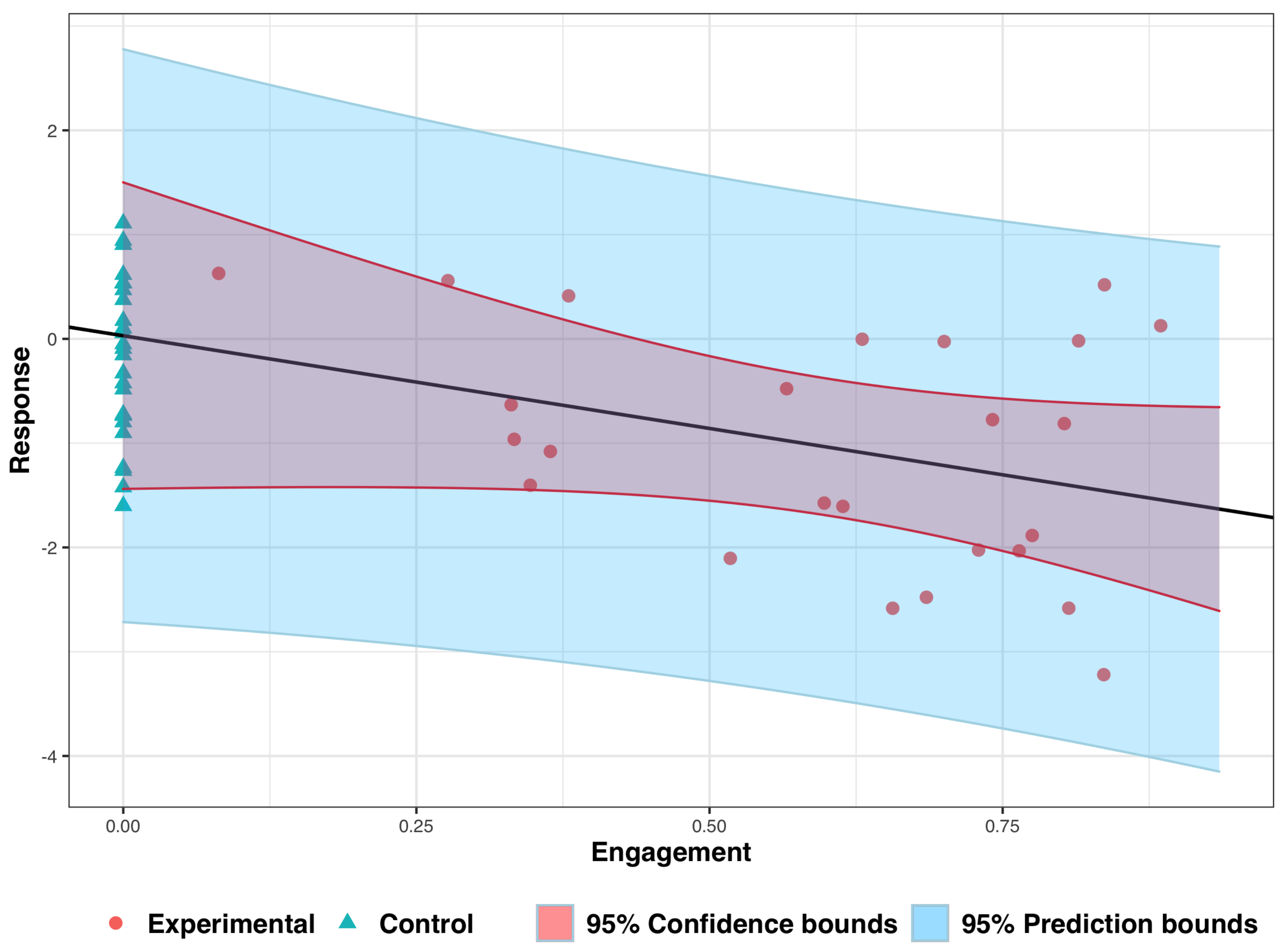
3. Analyzing Experimental Data: An Illustrative Example

Figure 1 visualizes a dataset from a hypothetical clinical trial with n = 50 subjects simulated from model (1) with parameters μ E = 0.5 , μ C = 0 , γ = 0.5 , and σ = 1 . Individual values of engagement in the experimental group were generated from a logit-normal distribution as follows: X = exp ( U ) 1 + exp ( U ) , where U N o r m a l log 0.6 0.4 , 1 . With this approach, we assure that X is between 0 and 1, with E ( X ) 0.6 and SD ( X ) 0.2 . The sample summary statistics for engagement were x ¯ E = 0.6 and S x x = 1.13 .
Let us analyze these data using ANCOVA, as described in Section 2.1. We have Y ¯ E = 1.04 , Y ¯ C = 0.18 , S x x = 1.13 , S x y = 31.12 , and thus γ ^ = S x y S x x = 1.78 8, μ ^ E = Y ¯ E γ ^ x ¯ E = 0.03 , μ ^ C = Y ¯ C = 0.18 , and σ ^ 2 = 0.89 9. The sample correlation between engagement and response in the experimental group is r = S x y S x x S y y = 0.34 .
The value of the t-statistic for testing H 0 : μ E μ C = 0 using Equation (6) is t = 0.346 , with the corresponding 2-sided p-value = 0.731, implying that μ E and μ C are not statistically different. The point estimate of μ E μ C is μ ^ E μ ^ C = 0.207 , and the corresponding 95% confidence interval is ( 1.00 , 1.41 ) , which covers both zero and the true value of the mean difference μ E μ C = 0.5 .
The value of the t-statistic for testing H 0 : γ = 0 using Equation (8) is t = 2.005 , with the corresponding two-sided p-value = 0.051 , a marginally significant result. The 95% confidence interval for γ is ( 3.56 , 0.01 ) .
The value of the t-statistic for testing H 0 : Δ x ¯ E = 0 using Equation (12) is t = 3.24 , with the corresponding two-sided p-value = 0.0022 , which indicates reasonably good evidence against H 0 . The 95% confidence interval for Δ x ¯ E is ( 1.40 , 0.33 ) , which covers the true value Δ x ¯ E = 0.5 0.5 × 0.60 = 0.8 .
The smallest level of engagement that leads to statistically significant difference between two groups can be found by solving an inequality for the upper limit of the 95% confidence interval for Δ x = ( μ E + γ x ) μ C ; that is: 0.03 1.78 x + 0.18 + 2.01 × 0.944 4 50 + ( x 0.6 ) 2 1.13 < 0 . The solution is 0.4533 < x < 207.74 , for which only the lower limit is relevant. Thus, we conclude that ∼46% is the smallest level of engagement required to obtain a statistically significant (using two-sided α = 0.05 ), larger response in the experimental group compared to the control.
A 95% confidence interval for the expected value of the response for a given level of engagement x is found as 0.03 1.78 x ± 2.01 × 0.944 2 50 + ( x 0.6 ) 2 1.13 . For instance, if a subject successfully completes 80% of the dCBT program ( x = 0.8 ), the 95% confidence interval for the mean response is obtained as ( 0.87 , 0.23 ) . A 95% prediction interval for a new observation Y ( x ) is found as 0.03 1.78 x ± 2.01 × 0.944 1 + 2 50 + ( x 0.6 ) 2 1.13 . For x = 0.8 , the 95% prediction interval is ( 2.4 , 1.77 ) .
Suppose an investigator decides to perform statistical inference using a two-sample t-test, as described in Section 2.2. They obtain Y ¯ E Y ¯ C = 1.04 + 0.18 = 0.86 , S p 2 = 0.946 , and the t statistic t = 0.86 0.946 × 4 / 50 = 3.15 , with the two-sided p-value = 0.0028 . (Note that for the ANCOVA approach the t-statistic was more extreme: t = 3.24 ; and the two-sided p-value was slightly smaller: p = 0.0022 , indicating greater evidence against H 0 ). A 95% confidence interval for Δ x ¯ E based on the two-sample t-test is ( 1.42 , 0.31 ) .
Overall, while the two-sample t-test leads to a similar conclusion as the ANCOVA test, the inference for the former approach is only limited to the contrast μ E + γ x ¯ E μ C , whereas ANCOVA allows investigators to address more research questions.

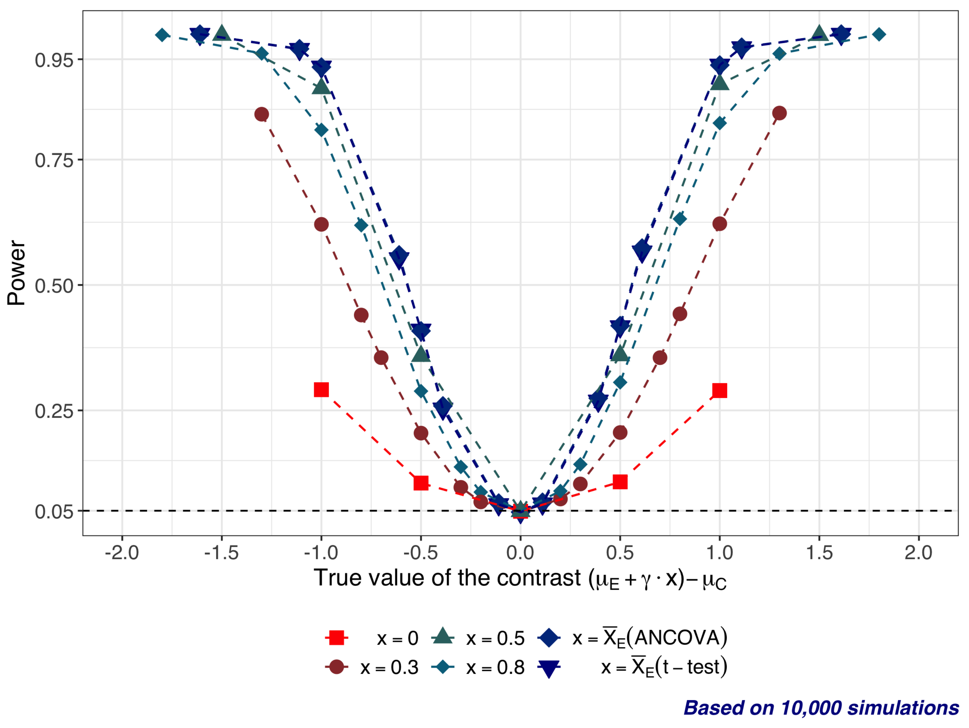
4. Statistical Properties of Significance Tests: A Simulation Study

To gain further insights into the properties of statistical tests described in Section 2, we ran Monte Carlo simulations under different experimental scenarios. We considered the following parameter values for the simulations:
  • μ C = 0 and μ E is in the range from −1 to 1; therefore Δ = μ E μ C = 1 , 0.5 , 0 , 0.5 , 1 .
  • γ (slope) is in the range from −1 to 1 ( γ = 1 , 0.5 , 0 , 0.5 , 1 ).
  • σ 2 = 1 .
  • n = 50 (25 subjects per arm).
  • All tests are 2-sided, with significance level α = 0.05 .
Engagement in the experimental group was simulated as a random sample of size 25 from a normal distribution with mean λ = 0.6 and standard deviation ξ = 0.2 . The sample summary statistics were x ¯ E = 0.62 and S x x = 1.38 , and these values were fixed throughout simulations.
For each experimental scenario defined by a combination of Δ , γ , σ 2 , and n, we consider testing H 0 : Δ x = 0 , where Δ x = Δ + γ x is the contrast between the combined effect of the novel CBT + dCBT engaged at level x and the effect of the control treatment using the ANCOVA test (12) for several pre-specified levels of engagement x, namely x = 0 , 0.3 , 0.5 , and 0.8 . Moreover, we consider testing H 0 : Δ x ¯ E = 0 , i.e., the significance of the difference between the effects of the experimental treatment at the average observed engagement x ¯ E = 0.62 and that of the control treatment. For the latter hypothesis, we consider two tests: the ANCOVA test (12) with x = x ¯ E = 0.62 and the two-sample t-test (17).
For each experimental scenario, the type I error rate and power of statistical tests were estimated based on 10,000 Monte Carlo simulations. For each simulation, outcome data were generated from model (1) with the chosen values of trial parameters. The proportion of simulations for which a given test yielded a statistically significant result was taken as a Monte Carlo estimate of type I error rate (or power).
Figure 2 shows the power patterns, which are plotted using different symbols for x = 0 (red square, ), x = 0.3 (brown circle, ), x = 0.5 (dark green triangle, ), x = 0.8 (dark green rhombus, ), x = 0.62 , ANCOVA test (dark blue rhombus, ), and x = 0.62 , two-sample t-test (dark blue inverted triangle, ). The x-axis displays the true values of the contrast Δ x = Δ + γ x . Note that several combinations of ( Δ , γ , x ) can yield the same value of Δ x . For instance, ( Δ , γ , x ) = ( 1 , 1 , 0 ) and ( Δ , γ , x ) = ( 0.5 , 1 , 0.5 ) correspond to Δ x = 1 . The y-axis displays the values of statistical power. For Δ x = 0 , the power is equal to 0.05 (type I error rate). For Δ x 0 , power > 0.05 . Clearly, the power is monotone increasing in | Δ x | .
One remarkable observation from Figure 2 is that the power is larger for values of x that are closer to the average observed engagement (which is equal to 0.62 in our example). This observation is in good correspondence with the theory, which posits that the value of the ANCOVA test statistic in Equation (12) is maximized (hence, maximizing the chance of obtaining a statistically significant result, i.e., achieving maximum power) for x = x ¯ E . For instance, compare the values of power for two different scenarios that yield Δ x = 1 : for ( Δ , γ , x ) = ( 1 , 1 , 0 ) , the power is 0.29, whereas for ( Δ , γ , x ) = ( 0.5 , 1 , 0.5 ) , the power is 0.89. Note that in these two scenarios we have the same value of the linear slope: γ = 1 , and in the first scenario the value of Δ is more extreme ( Δ = 1 ) than in the second scenario ( Δ = 0.5 ). Yet, the value of power in the second scenario (0.89) is much larger than that in the first scenario (0.29). Such a drastic difference in power is due to the fact that in the second scenario we are testing a contrast at the level of engagement x = 0.5 that is much closer to the average observed level of engagement ( x ¯ E = 0.62 ) than the level of engagement in the first scenario ( x = 0 ).
Of note, Δ x = 1 can be also obtained for Δ = 1 , γ = 0 and any value of x. In this case, the linear slope γ is zero, and the mean treatment difference is equal to −1 for any level of engagement x. The corresponding values of power range from 0.29 (for x = 0 ) to 0.93 (for x = x ¯ E = 0.62 ).
As another example, consider ( Δ , γ , x ) = ( 0.5 , 1 , 0.5 ) for which Δ x = 1 , and ( Δ , γ , x ) = ( 1 , 1 , 0.3 ) for which Δ x = 1.3 . Despite that in the latter case the treatment difference is more extreme ( Δ = 1 and Δ x = 1.3 ) than in the former case ( Δ = 0.5 and Δ x = 1 ), the value of power in the latter case is smaller (0.84) than that in the former case (0.89). This is because the engagement level in the latter case ( x = 0.3 ) is more distant from the average observed level of engagement ( x = x ¯ E = 0.62 ) than the engagement level in the former case ( x = 0.5 ).
Overall, based on the results from Figure 2 we highlight two important observations: 1) The level of engagement at which the group comparison is made affects statistical power. 2) The values of power of the ANCOVA test and the two- sample t-test are very close. This implies that both ANCOVA and a two-sample t-tests are appropriate for the inference on treatment difference at the average observed level of engagement.
These findings highlight the importance of clearly formulating study objectives, because sample size and power depend on the choice of the primary estimand. In what follows, we discuss some statistical considerations that can be useful at the study planning stage.

5. Design Aspects

5.1. Optimality of Equal Allocation

Throughout the chapter we assumed the trial is designed using equal (1:1) allocation, with n participants equally randomized between experimental and control groups ( n / 2 per group). We now provide a formal justification for optimality of equal allocation in this setting.
Suppose n E = n ρ subjects are assigned to the experimental group and n C = n ( 1 ρ ) subjects are assigned to the control group, where 0 < ρ < 1 is the allocation proportion. We are interested in the value of ρ that minimizes the variance of the treatment contrast Δ x = ( μ E + γ x ) μ C for some chosen fixed value of x. This goal is closely related to the maximization of statistical power of testing H 0 : Δ x = 0 . We have Δ ^ x = Y ¯ E + γ ^ ( x x ¯ E ) Y ¯ C , and
var Δ ^ x = σ 2 n ρ + σ 2 ( x x ¯ E ) 2 S x x + σ 2 n ( 1 ρ ) ,
which is minimized for ρ = 1 / 2 , the equal allocation.

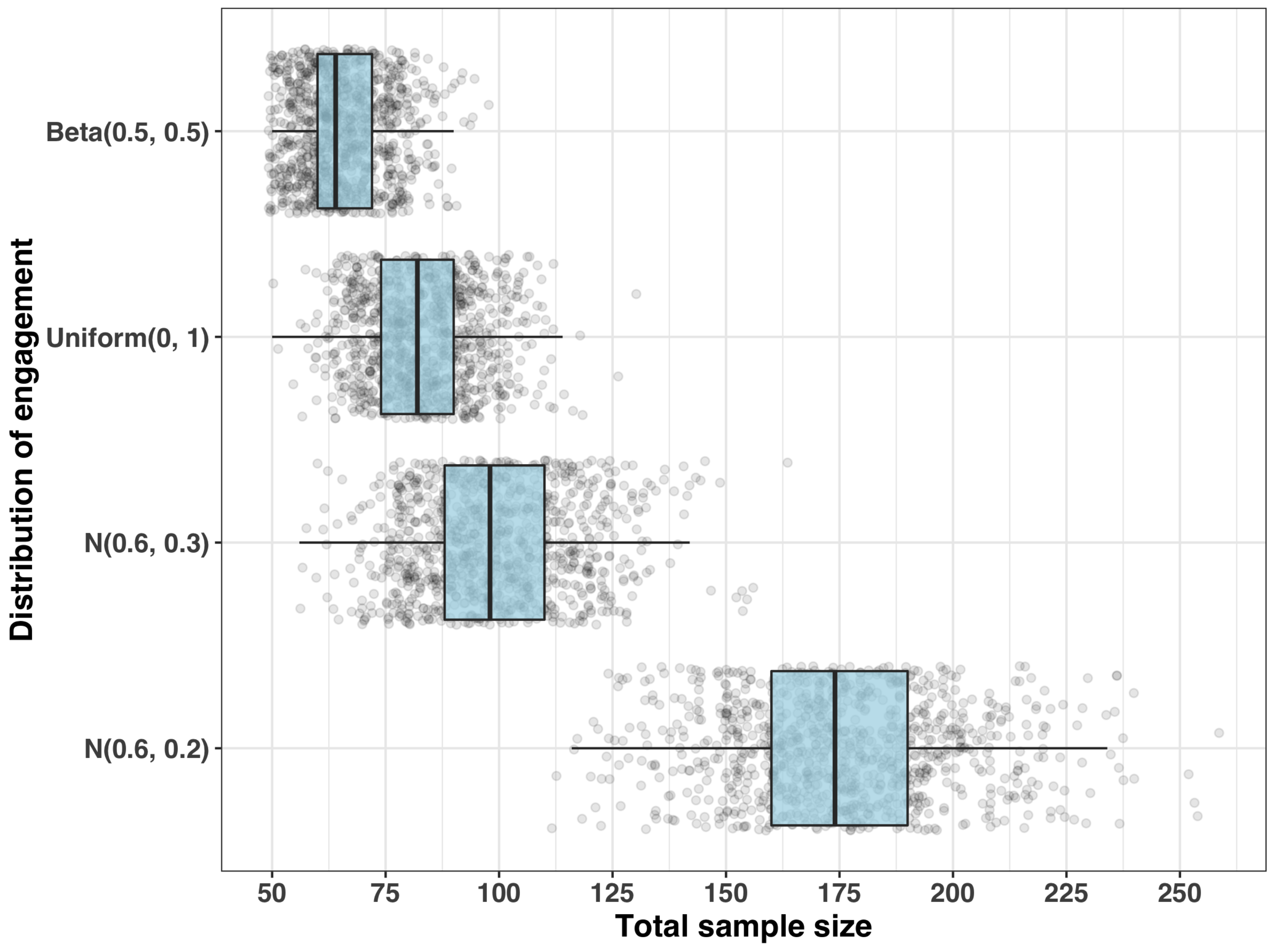
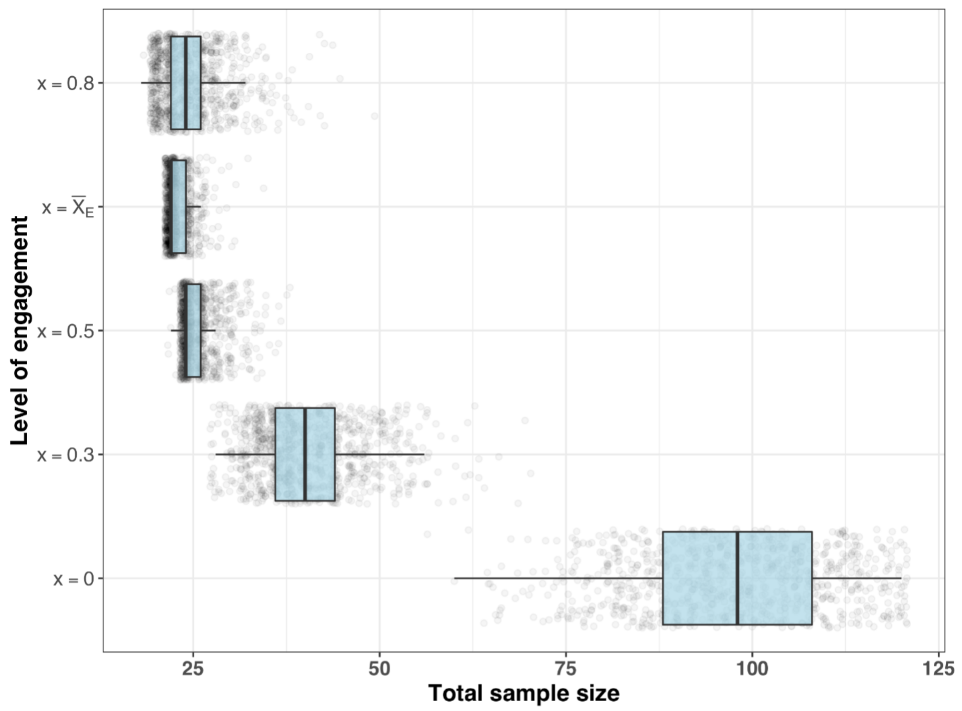
5.2. Sample Size Considerations

Suppose we are interested in testing H 0 : Δ 0 = 0 , which posits that there is no difference between the effects of the novel CBT alone and the control intervention, and we want to determine the sample size to achieve some desired level of statistical power for this test. The sample size is determined as a function of several design parameters whose values must be pre-specified upfront:
  • α = chance of a false positive result;
  • β = chance of a false negative result;
  • Δ ˜ 0 = the “clinically relevant” mean treatment difference that we would not like to miss;
  • σ = the presumed standard deviation of the primary outcome.
Assuming equal (1:1) allocation, the total sample size n is determined to satisfy two major conditions: α = Pr ( Reject H 0 | Δ 0 = 0 ) and 1 β = Pr ( Reject H 0 | Δ 0 = Δ ˜ 0 ) . Using the test statistic in Equation (6), H 0 is rejected if | t | > t α / 2 , n 3 . One difficulty is that the distribution of this test statistic depends on engagement—via x ¯ E and S x x —that are calculated for a particular value of the sample size, using individual engagement values that are unknown upfront. Therefore, we have a conundrum: for sample size planning we need summary statistics of engagement, which are derived from an experiment of a given size. If we have some prior knowledge on the probability distribution of engagement, we can use it to calibrate the sample size for a future study. A sensible approach for this purpose is Monte Carlo simulation. There are two major steps in the simulation process that should be implemented to calibrate the requisite sample size and quantify the associated uncertainty.
  • Step 1: Sample size for a given set of engagement measurements
Suppose, based on a pilot study, it is plausible to assume that individual values of engagement follow a normal distribution with mean λ and standard deviation ξ . We simulate a vector of engagement values: X = ( X 1 , , X M ) , where X i i . i . d . N ( λ , ξ 2 ) and M is some pre-specified large positive integer (say, M = 200 ). Let m M denote the sample size for the experimental group (the total sample size is n = 2 m ). For a given m (say, m = 25 ) we take the first m components of the vector X , i.e., X ( m ) = ( X 1 , , X m ) , calculate x ¯ E = 1 m i = 1 m X i and S x x = i = 1 m ( X i x ¯ E ) 2 . Next, we run 10,000 simulations to generate datasets from model (1) with the chosen parameter values ( μ E , μ C , γ , σ ) , total sample size n = 2 m , keeping fixed within each simulation run the individual values of engagement and treatment assignment indicators. For each simulation, the test statistic is computed using Equation (6), and the test decision is recorded (reject H 0 , if | t | > t α / 2 , 2 m 3 ; or fail to reject H 0 , if | t | t α / 2 , 2 m 3 . The proportion of simulation runs that lead to rejection of H 0 is taken as a Monte Carlo estimate of power for the given m.
The above procedure is repeated for different values of m (say, m = 25 , 26 , , M ), and for each m the simulated power is obtained. The smallest sample size n = 2 m for which simulated power is equal to or exceeds the target level 1 β provides the requisite sample size. A plot of power (y-axis) vs. sample size (x-axis) can be helpful to visualize the n’s that yield different values of power (80%, 90%, etc.)
  • Step 2: Distribution of the requisite sample size
The described Step 1 provides a single value of the sample size to achieve power = 1 β . However, this sample size is obtained for a fixed set of engagement values. Since in practice there is uncertainty around the engagement (we assume it can be quantified using N ( λ , ξ 2 ) distribution), we can repeat the entire procedure described in Step 1 (say, 1000 times) to obtain a distribution of the requisite sample size. An experimenter may then decide to use some percentile of this distribution (say, 80th percentile), to ensure that their experiment has the desired level of power = 1 β , with reasonably high confidence, for the chosen values of trial parameters. A histogram or a box-plot of the simulated distribution of the sample size can provide valuable insights into the required sample size and the associated uncertainty.
Figure 3 displays box-plot distributions of the smallest sample size to achieve 80% power of the test using 2-sided α = 5 % . Individual responseses were generated from model (1) with parameters μ E = 1 , μ C = 0 , γ = 0.5 , and σ = 1 . Four different distributions of engagement were considered:
(i)
X B e t a ( 0.5 , 0.5 ) , which has mean = 0.5 and SD 0.354 ;
(ii)
X U n i f o r m ( 0 , 1 ) , which has mean = 0.5 and SD 0.289 ;
(iii)
X N o r m a l with mean = 0.6 and SD = 0.3 ; and
(iv)
X N o r m a l with mean = 0.6 and SD = 0.2 .
For each of the four engagement patterns, simulations were performed as described above. In Step 1, we ran 10,000 simulations to obtain empirical power for the total sample size n = 2 m , where m = 25 , 26 , , 200 , and used the smallest n for which empirical power 80 % as an estimate of the required sample size. In Step 2, 1000 replications of Step 1 were performed.
From Figure 3, several important observations can be made. First, the requisite sample size is smaller if the underlying distribution of engagement is more variable. This makes good sense, because from Equation (4), var μ ^ E μ ^ C = σ 2 4 n + x ¯ E 2 S x x , and larger sample variance of engagement ( S x x term in the denominator) implies lower value of var μ ^ E μ ^ C , which leads to a larger absolute value of the t-statistic in Equation (6), and therefore higher power of the test. Second, there is uncertainty in the requisite sample size, and this uncertainty is smaller if the engagement is more variable.
Table 1 shows the summary statistics for the sample size distributions from Figure 3. Suppose it is plausible to assume that individual engagement values are uniformly distributed over the interval (0, 1), and an investigator wants to be 80% (or 90%) confident that the experiment has 80% statistical power for the chosen trial parameters ( μ E = 0 , μ C = 1 , γ = 0.5 , and σ = 1 ). Then, the required total sample size is n = 92 (or 98). On the other hand, if it is plausible to assume that engagement follows a normal distribution with mean 0.6 and standard deviation 0.2, and we want to be 80% (or 90%) confident that the experiment has 80% statistical power, the required sample size is n = 194 (or 206).
Note that if we consider another research hypothesis, e.g., H 0 : Δ x = 0 for some x > 0 , then the required sample size will be different. For instance, if we wish to test H 0 : Δ x ¯ E = 0 , then we can follow a conventional approach to sample size determination using the two-sample t-test, which requires no upfront knowledge on engagement. In the considered example (assuming between-group mean difference at the average engagement in the experimental group is equal to −1 common standard deviation σ = 1 ; two-sided significance level α = 5 % ; and power = 80%), a sample size n = 34 (17 per group) is required to detect the statistically significant group difference using two-sample t-test, which is much lower than the sample sizes presented in Table 1 and Figure 3.
  • Sample size requirements for different estimands
It is instructive to explore sample size requirements for research hypotheses involving different estimands. Let us assume that the underlying distribution of engagement is normal with mean = 0.6 and SD = 0.3 , and the true model parameters μ E = 1 , μ C = 0 , γ = 0.5 , and σ = 1 . We consider testing H 0 : Δ x = 0 for x = 0 , 0.3 , 0.5 , 0.8 , and x = x ¯ E .
Figure 4 shows box-plot distributions of the smallest sample size to achieve 80% power (with a two-sided significance level α = 5 % ) of the test of H 0 : Δ x = 0 , and Table 2 shows the corresponding summary statistics. As expected, the sample size is smallest when x = x ¯ E . By choosing n = 24 (12 subjects per arm), we can be 90% confident that our trial has 80% power to reject H 0 : Δ x ¯ E = 0 at the 5% significance level. For other values of x, the requisite sample size is larger. For instance, for x = 0.5 , to achieve 80% power with 90% confidence, one must choose n = 30 . The similar number for x = 0.3 is n = 50 , and for x = 0 it is n = 114 .
Note that, in general, when consider testing H 0 : Δ x = 0 , the sample size determination involves the value of Δ x = ( μ E + γ x ) μ C under the alternative, which necessitates the choice of μ E , μ C , γ , and x. In addition, we would need to make an assumption on the underlying distribution of engagement, to account for an inherent uncertainty in the engagement pattern. By contrast, if the objective is to test significance of the contrast between the effect of the experimental treatment at the average observed value of engagement and the control, fewer assumptions are needed; in particular, only the value of the clinically meaningful mean difference (without assumptions on γ , x, and engagement distribution) would suffice.
To draw a parallel between the results presented in Table 2 and the conventional sample size calculation, note that for x = x ¯ E = 0.6 , μ E = 1 , μ C = 0 , and γ = 0.5 , we have a mean treatment difference Δ x = 1 0.5 × 0.6 = 1.3 . The required sample size for a two-sample t-test with parameters Δ = 1.3 , σ = 1 , α = 0.05 , and 1 β = 0.8 can be obtained using standard statistical software, and it is n 22 (11 subjects per arm). Notice that n = 22 this is the median sample size (Q50) corresponding to x = x ¯ E in Table 2. In other words, for the chosen parameters, a trial design with n = 22 subjects has 80% power with 50% probability. If we want to achieve 80% power with 90% probability, the sample size should be increased to n = 24 (which is Q90 corresponding to x = x ¯ E in Table 2). Moreover, if we are interested in performing statistical testing at other levels of engagement (i.e., x x ¯ E ), then the sample size should be further increased to maintain 80% power with due level of confidence.
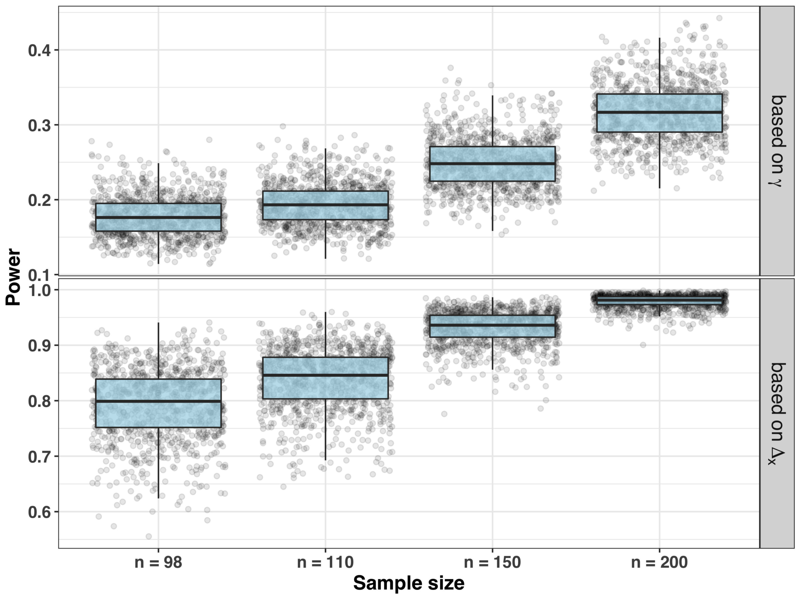
  • Sample size and power for testing significance of the slope
A sample size that may be viewed as sufficient for the purpose of treatment comparison may not be sufficient for other objectives, such as testing significance of the linear slope γ . Consider the same experimental setting as above (underlying distribution of engagement is normal with mean = 0.6 and SD = 0.3 , and the model parameters are μ E = 1 , μ C = 0 , γ = 0.5 , and σ = 1 ).
Figure 5 shows box-plot distributions of power of the test in Equation (8) testing significance of the slope: H 0 : γ = 0 (top panel) and similar distributions of the test of mean difference: H 0 : Δ 0 = 0 (bottom panel) for the four choices of the sample size ( n = 98 , 110 , 150 , and 200 ). With n = 200 , the power for testing H 0 : Δ 0 = 0 is > 90 % ; however, the power for testing significance of the slope is in the range 20–45%.

6. Conclusions and Future Work

To obtain valid results for an RCT, both the study design and the model for statistical analysis must be chosen judiciously. If the primary outcomes in the two groups are normally distributed with a common standard deviation, then a two-sample t-test is appropriate for testing the significance of the treatment mean difference. Its application rests on an important assumption that the average values of patient characteristics are approximately equal in the experimental and control groups (which is a reasonable assumption for a randomized trial).
In many clinical trials, there are important covariates that are correlated with a primary outcome. Adjusting for these covariates in the analysis can improve precision for estimating treatment effects. For a linear model with normal error terms, ANCOVA is a valid and well-established approach to analyze RCT data, and, in fact, it is advocated by the health authorities [14,15]. When properly applied, ANCOVA leads to the minimum variance of unbiased estimates of the model parameters, and it is potentially more powerful for testing treatment difference than a simple (unadjusted) analysis using a two-sample t-test. Furthermore, ANCOVA gains in efficiency are more pronounced for larger values of correlation between the primary outcome and the covariates of interest.
In the present paper, we explored these ideas in a context of an RCT evaluating cognitive behavioral therapies, assuming that engagement (quantified as the percentage of successfully completed trainings, measured without error) is an influential covariate. Our findings are in good correspondence with the already available statistical theory. One key contribution of our paper (which, to our knowledge, has not been addressed previously) is the investigation of statistical power and sample size of ANCOVA for different levels and patterns of engagement. A two-sample t-test matches one specific goal of ANCOVA, namely testing significance of the treatment difference at the average level of engagement observed in the study. In this case, the two-sample t-test and ANCOVA generally yield similar power (which can be observed from our simulation results in Figure 2). However, the average level of engagement is not known upfront, and investigators may wish to compare treatment effects at several levels of engagement (including the average to be observed in the study), to enable generalization of the RCT results to a broader population. Our simulation results demonstrate that larger sample sizes may be required to achieve a given value of power than one would typically expect. The pattern of engagement, the level of engagement at which the treatment contrast is estimated, the value of the linear slope, the mean treatment effects and the standard deviation of the response have an impact on statistical power in this case. Therefore, it is essential that the primary research question is clearly formulated upfront to ensure that the experiment is adequately powered.
While our considered approach in this paper was for a rather simple model (a single covariate representing engagement in the experimental group, measured on a continuous scale from 0 to 1), it captures an essential feature of experiments evaluating complex interventions—the need for considering patient engagement in both the design and analysis of the experimental data. However, our assumed model can be challenged on a number of grounds. First, it is rather stringent and it may not hold on the boundary when the engagement is equal to zero. Formal statistical tests may be required for checking the plausibility of this assumption and a model-robust inference may be necessary at the analysis stage. We designate this as an important problem and defer it to the future work. Second, the formulation of a model adequately describing the relationship between the primary endpoint, treatment, engagement, and possibly other factors is a major problem in itself. It will depend on the disease area, the target patient population, the mechanism of action of an experimental therapy, etc. Product developers and clinical investigators should work closely with statisticians to build scientifically sound models and test/validate them in carefully designed experiments. These considerations merit further investigation, but they are beyond the scope of the present work.
We would like to conclude this paper by outlining some directions for future research. In the present work, we considered engagement as a covariate, and it was assumed to be measured without error. All estimates, standard errors, tests of hypotheses, and confidence and prediction intervals were obtained based on this assumption. Technically, since data on engagement is acquired after randomization, it is affected by treatment and should be regarded as a response. If we regard both engagement (X) and response (Y) as random variables, then different approaches to inference, such as error-in-variables regression models [16,17] should be considered. As one of the reviewers pointed out, it may be more appropriate to discuss patient engagement in the context of mediation analysis instead of covariate adjustment. An approach to mediation analysis when a continuous mediator is measured with error and the outcome follows a generalized linear model was described in the reference [18]. This approach may be also useful in the RCTs of digital mental health interventions, and we defer this to the future work.
Another important extension of the present work is the investigation of more complex statistical models defining the links among treatment, engagement, response, and possibly other factors. For instance, longitudinal models with repeated measurements at multiple visits, nonlinear models, and models with more than one covariate may provide more accurate descriptions of the phenomena of interest. Multiple ingredients of a CBT (individually or in combination) may have an impact on the response, which should be accounted for in both the design and the analysis. One recent paper [9] investigated the relationship between patient engagement and depressive symptoms among people with HIV based on data from a 3- month RCT comparing an mHealth intervention versus a wait-list control group. The authors used latent growth curve models to link patient engagement and depressive symptoms at multiple time points, up to 3 months of the mHealth intervention. Such an approach holds promise and warrants further consideration.
In our work, we assumed engagement is measured for subjects in the experimental group but not in the control group. However, in many settings the engagement is observed in both experimental and control groups; e.g., one may have the control app as “mindfulness only”, whereas the experimental app may be “mindfulness + diet + weight loss”. In this case, engagement is measurable in both groups, and different modeling strategies have to be considered.
Recently, machine learning techniques have been applied to understand patterns of engagement with internet-delivered CBTs [19]. These approaches can help identify different subtypes of patients that engage differentially with the digital interventions, and this may enable more personalized approaches to treatment. Incorporating machine learning tools in the design and analysis of RCTs of dCBTs seems to be a valuable approach that merits further investigation.

Author Contributions

Conceptualization: O.S. and Y.R.; methodology: O.S. and Y.R.; software: Y.R.; validation: O.S.; writing—original draft preparation: O.S.; writing—review and editing: O.S. and Y.R. All authors have read and agreed to the published version of the manuscript.

Funding

This research received no external funding.

Institutional Review Board Statement

Not applicable.

Informed Consent Statement

Not applicable.

Data Availability Statement

All results in this paper are based on simulated data. The computer code is fully documented and available from the second author upon request.

Acknowledgments

The authors are grateful to Brian P. Smith and the three anonymous referees for their review and feedback that helped improve the manuscript.

Conflicts of Interest

The authors declare no conflict of interest.

References

  1. Marsch, L.A. Sector perspective: Digital therapeutics in behavioral health. In Digital Therapeutics: Scientific, Statistical, Clinical and Regulatory Development Aspects, 1st ed.; Sverdlov, O., vam Dam, J., Eds.; CRC Press: Boca Raton, FL, USA, 2022. [Google Scholar]
  2. Sverdlov, O.; van Dam, J.; Hannesdottir, K.; Thornton-Wells, T. Digital Therapeutics: An Integral Component of Digital Innovation in Drug Development. Clin. Pharmacol. Ther. 2018, 104, 72–80. [Google Scholar] [CrossRef] [PubMed]
  3. Espie, C.A.; Henry, A.L. Designing and delivering a DTx clinical research program: No need to re-invent the wheel. In Digital Therapeutics: Scientific, Statistical, Clinical and Regulatory Development Aspects, 1st ed.; Sverdlov, O., van Dam, J., Eds.; CRC Press: Boca Raton, FL, USA, 2022; Chapter 4. [Google Scholar]
  4. Chung, J.Y. Digital therapeutics and clinical pharmacology. Transl. Clin. Pharmacol. 2019, 27, 6–11. [Google Scholar] [CrossRef] [PubMed] [Green Version]
  5. Yardley, L.; Spring, B.J.; Riper, H.; Morrison, L.G.; Crane, D.H.; Curtis, K.; Merchant, G.C.; Naughton, F.; Blandford, A. Understanding and Promoting Effective Engagement With Digital Behavior Change Interventions. Am. J. Prev. Med. 2016, 51, 833–842. [Google Scholar] [CrossRef] [PubMed] [Green Version]
  6. Ghaemi, S.N.; Sverdlov, O.; van Dam, J.; Campellone, T.; Gerwien, R. A Smartphone-Based Intervention as an Adjunct to Standard-of-Care Treatment for Schizophrenia: Randomized Controlled Trial. JMIR Form. Res. 2022, 6, e29154. [Google Scholar] [CrossRef] [PubMed]
  7. Truzoli, R.; Reed, P.; Osborne, L.A. Patient expectations of assigned treatments impact strength of randomised control trials. Front. Med. 2021, 8, 648403. [Google Scholar] [CrossRef] [PubMed]
  8. Montgomery, S.A.; Åsberg, M. A New Depression Scale Designed to be Sensitive to Change. Br. J. Psychiatry 1979, 134, 382–389. [Google Scholar] [CrossRef] [PubMed]
  9. Zeng, Y.; Guo, Y.; Li, L.; Hong, Y.A.; Li, Y.; Zhu, M.; Zeng, C.; Zhang, H.; Cai, W.; Liu, C.; et al. Relationship Between Patient Engagement and Depressive Symptoms Among People Living with HIV in a Mobile Health Intervention: Secondary Analysis of a Randomized Controlled Trial. JMIR mHealth uHealth 2020, 8, e20847. [Google Scholar] [CrossRef] [PubMed]
  10. Palmier-Claus, J.E.; Ainsworth, J.; Machin, M.; Barrowclough, C.; Dunn, G.; Barkus, E.; Rogers, A.; Wykes, T.; Kapur, S.; Buchan, I.; et al. The feasibility and validity of ambulatory self-report of psychotic symptoms using a smartphone software application. BMC Psychiatry 2012, 12, 172. [Google Scholar] [CrossRef] [PubMed] [Green Version]
  11. Kreyenbuhl, J.; Record, E.J.; Himelhoch, S.; Charlotte, M.; Palmer-Bacon, J.; Dixon, L.B.; Medoff, D.R.; Li, L. Development and Feasibility Testing of a Smartphone Intervention to Improve Adherence to Antipsychotic Medications. Clin. Schizophr. Relat. Psychoses 2019, 12, 152–167. [Google Scholar] [CrossRef] [PubMed]
  12. Bucci, S.; Barrowclough, C.; Ainsworth, J.; Machin, M.; Morris, R.; Berry, K.; Emsley, R.; Lewis, S.; Edge, D.; Buchan, I.; et al. Actissist: Proof-of-concept trial of a theory-driven digital intervention for psychosis. Schizophr. Bull. 2018, 44, 1070–1080. [Google Scholar] [CrossRef] [PubMed]
  13. Myers, R.H. Classical and Modern Regression with Applications, 2nd ed.; Duxbury Press: London, UK, 1990. [Google Scholar]
  14. European Medicines Agency (EMA). Guideline on Adjustment for Baseline Covariates in Clinical Trials; EMA/CHMP/295050/2013, 26 February 2015. Available online: https://www.fda.gov/media/148910/download (accessed on 9 May 2022).
  15. U.S. Food & Drug Administration. Adjusting for Covariates in Randomized Clinical Trials for Drugs and Biological Products; Draft Guidance for Industry, May 2021. Available online: https://www.fda.gov/regulatory-information/search-fda-guidance-documents/adjusting-covariates-randomized-clinical-trials-drugs-and-biological-products (accessed on 9 May 2022).
  16. Fuller, W.A. Measurement Error Models; Wiley: New York, NY, USA, 1987. [Google Scholar]
  17. Carroll, R.J.; Ruppert, D.; Stefanski, L.A.; Crainiceanu, C.M. Measurement Error in Nonlinear Models. A Modern Perspective, 2nd ed.; Chapman and Hall/CRC: Boca Raton, FL, USA, 2006. [Google Scholar]
  18. Valeri, L.; Lin, X.; VanderWeele, T.J. Mediation analysis when a continuous mediator is measured with error and the outcome follows a generalized linear model. Stat. Med. 2014, 33, 4875–4890. [Google Scholar] [CrossRef] [PubMed]
  19. Chien, I.; Enrique, A.; Palacios, J.; Regan, T.; Keegan, D.; Carter, D.; Tschiatschek, S.; Nori, A.; Thieme, A.; Richards, D.; et al. A Machine Learning Approach to Understanding Patterns of Engagement with Internet-Delivered Mental Health Interventions. JAMA Netw. Open 2020, 3, e2010791. [Google Scholar] [CrossRef] [PubMed]
Figure 1. An example of experimental data from a trial of n = 50 subjects (25 per group). Group 1 (experimental) observations are red circles; group 2 (control) observations are green triangles. ANCOVA-fitted linear regression (solid black line) is μ ^ E + γ ^ x .
Applsci 12 04952 g001
Figure 2. Statistical power for testing H 0 : Δ x = 0 , where Δ x = Δ + γ x , for different combinations of Δ = ( 1 , 0.5 , 0 , 0.5 , 1 ) , γ = ( 1 , 0.5 , 0 , 0.5 , 1 ) , and x = ( 0 , 0.3 , 0.5 , 0.62 , 0.8 ) . It is assumed that n = 50 (25 subjects per arm) and outcomes are generated from model (1) with parameters μ E = Δ in the range from −1 to 1; μ C = 0 ; γ in the range from −1 to 1; and σ = 1 .
Applsci 12 04952 g002
Figure 3. Distributions of the sample size to achieve 80% power of ANCOVA t-test of H 0 : Δ 0 = 0 using 2-sided α = 5 % . Responses were simulated from model (1) with μ E = 1 , μ C = 0 , γ = 0.5 , and σ = 1 . Four different distributions of engagement were considered (top to bottom): Beta(0.5,0.5); Uniform(0,1); Normal with mean = 0.6 and standard deviation ( SD ) = 0.3 ; and N o r m a l with mean = 0.6 and SD = 0.2 .
Applsci 12 04952 g003
Figure 4. Distributions of the sample size to achieve 80% power of ANCOVA t-test of H 0 : Δ x = 0 (using 2-sided α = 5 % ) for x = 0 , 0.3 , 0.5 , 0.8 , and x = x ¯ E . Responses were simulated from model (1) with μ E = 1 , μ C = 0 , γ = 0.5 , and σ = 1 . Engagement values were simulated from a normal distribution with mean = 0.6 and SD = 0.3 .
Applsci 12 04952 g004
Figure 5. Distributions of power of the test of significance of the slope (top panel) and power of ANCOVA t-test of H 0 : Δ 0 = 0 (bottom panel). Both tests used a two-sided significance level α = 5 % (two-sided). Responses were simulated from the model (1) with μ E = 1 , μ C = 0 , γ = 0.5 , and σ = 1 . Engagement values were simulated from a normal distribution with mean = 0.6 and SD = 0.3 .
Applsci 12 04952 g005
Table 1. Summary statistics for the total sample size distributions (cf. Figure 3).
Total Sample Size (n)
Distribution of Engagement ( X )Q50Q80Q90Max
B e t a ( 0.5 , 0.5 ) 64747898
U n i f o r m ( 0 , 1 ) 829298130
N o r m a l ( 0.6 , SD = 0.3 ) 98112120164
N o r m a l ( 0.6 , SD = 0.2 ) 174194206258
Q50 = median; Q80 = 80th percentile; Q90 = 90th percentile; Max = maximum.
Table 2. Summary statistics for the total sample size distributions (cf. Figure 4).
Total Sample Size (n)
x Q50Q80Q90
098110114
0.3404650
0.5242630
x ¯ E 222424
0.8242830
Q50 = median; Q80 = 80th percentile; Q90 = 90th percentile.
Publisher’s Note: MDPI stays neutral with regard to jurisdictional claims in published maps and institutional affiliations.

