Design of an Eye-in-Hand Smart Gripper for Visual and Mechanical Adaptation in Grasping

Featured Application

The eye-in-hand adaptive gripper can be used in intelligent manufacturing applications. With its eye-in-hand feature and adaptive mechanism, the smart gripper can offer both visual and mechanical adaption in grasping objects of any shape. It also offers automatic identification and tracking of a moving object with its vision servoing feature.

Abstract

With the advancement of robotic technologies, more and more tasks in industrial and commercial applications rely on the use of robots to assist or even replace humans. To fulfill the needs of grasping and handling different objects, the development of a universal grasping device acting as an end-effector to a robotic manipulator has been one of the main robotic research and development focuses. Therefore, this study was aimed at the development of a general robotic gripper with three fingers for adaptive actuation and an eye-in-hand vision system. With the adaptive actuation feature, each finger of the robotic gripper contained multiple degrees of freedom that allowed the finger to change its shape to wrap around an object’s geometry adaptively for stable grasping. With the eye-in-hand configuration in the adaptive gripper, it offered advantages including occlusion avoidance, intuitive teleoperation, imaging from different angles, and simple calibration. This study proposed and integrated a plug-and-play gripper module, controller module, and visual calculation module all in the model smart gripper, of which the gripper was further validated by calibrated experiments. The proposed gripper featured mechanical adaptation and visual servoing adaptivity to achieve 100% gripping success rate when gripping a moving target of any shape that was carried by conveyor belt with moving speed less than 70 mm/s. By integrating mechanical and visual adaptivity, the proposed gripper enabled the inclusion of intelligence in robotic applications and can further be used in smart manufacturing and intelligent robotic applications.

1. Introduction

With the advancement of technology, robots have been widely incorporated into industrial, commercial, and even home applications. For applications in daily life or smart manufacturing environments, a robotic gripper that can universally grasp objects is of utmost importance. Owing to the needs of high accuracy, high repeatability, and strong gripping force, an industrial robotic gripper is commonly designed to possess a single-degree-of-freedom actuation. Despite the aforementioned advantages, it is difficult to adapt to different objects. As such, to maximize the flexibility in grasping, changing the adaptors in this single-degree-of-freedom gripper is necessary.

Currently, the most dexterous gripper available is the human hand, and its flexibility is too hard to achieve by a robotic gripper. To mimic the characteristics of a human hand, J. Jin et al. designed a humanoid hand with multiple degrees of freedom and five fingers [1], and Z. Kappassov et al. also developed a 3D-printed humanoid hand control with five fingers and four motors embedded in the hand [2]. They attempted to design a humanoid robotic hand to imitate human motion.

Although a humanoid gripper has good flexibility, its accuracy and payload capacity are limited. G. Li and W. Zhang used springs and belts to control multiple finger joints by using a single motor to build an under-actuated gripper [3]. This under-actuated gripper adapted the surface of an object by the force-limit characteristics of a driven chain, during which certain finger joints would stop while the others kept moving to adaptively cover the object. To reduce the number of actuation elements, such as motors, in a robotic gripper, K. Telegenov et al. proposed an adaptive structure that contained redundant degrees of freedom [4]. This gripper utilized a single driving source to control its finger, which consisted of linkage structures with multiple degrees of freedom. L. Birglen and C. M. Gosselin proposed a gripper finger that used multiple four-bar linkages in series [5] to reduce the number of driving sources while maintaining or even improving the adaptability of the gripper. Based on this design concept, they attempted to derive mathematical functions for each adaptive gripper finger joint [6]. Conversely, L. Birglen and C. M. Gosselin reported that the adaptability of the adaptive gripper is affected by external forces applied to the structure, which eventually led to bending of the finger structures [7]. To properly design an adaptive gripper, a design concept with multiple redundant degrees of freedom was investigated in our previous study [8]. To take it further, systemic and detailed analytical parameter studies and integration with visually adaptive algorithms are conducted and examined in this paper. Experimental validations were conducted by prototyping an eye-in-hand adaptive three-finger robotic gripper through mechatronics integration.

In addition to the mechanical-adaptive feature, robotic arms with computer vision systems are widely used in pick-and-place and visual-tracking control applications. Three types of camera installation are typically used, as illustrated in Figure 1. The first type is an eye-to-hand system, in which the frames of the camera and gripper are in different coordinate systems. The second type is the eye-on-hand system, where the camera and gripper are mounted at the end of the manipulator, but the coordinate system of the camera is offset from that of the gripper. The third type is the eye-in-hand system, where the camera and gripper are again mounted at the end of the manipulator but share the same coordinate system. In other words, the camera is part of the gripper module in the eye-in-hand configuration. For an eye-to-hand system, the camera’s view can be obstructed by another object that is neither part of the target nor the arm of the manipulator itself. However, eye-on-hand and eye-in-hand systems can solve this problem because the camera can move along with the manipulator.

The difference between the eye-on-hand and the eye-in-hand configurations is primarily on the camera’s mounting position. In eye-in-hand configuration, the camera shares the same coordinate system with the gripper. In eye-on-hand configuration, the camera and the gripper are located and described by different coordinates in which configuration of the so-called out-sight problem may occur when the camera is close to the object. This problem is graphically illustrated in Figure 2, where the size of the target object is set as a ten-by-ten-centimeter square, and the offset between eye-in-hand and eye-on-hand coordinate is 15 cm. As the distance between the camera and the target object changes, in particular when the distance is less than 30 cm, the target object becomes out of view in eye-on-hand configuration. Nevertheless, such a problem does not occur in the eye-in-hand configuration, as it is still available regardless of the relative position and distance between the camera and the gripper.

In R. Barth’s paper, the main purpose was to find a crop-like berry, which was behind some leaves, and collected by a robot arm with a camera on the manipulator [9]. The camera can avoid the leaves and find the crop by moving the manipulator using an eye-on-hand system. In addition to R. Barth’s paper, a substantial number of research studies have used the eye-on-hand configuration to avoid occlusion [10,11,12,13]. In fact, both eye-in-hand and eye-on-hand configurations can perform intuitive teleoperation tasks using high-DOF servo-manipulators [14]. The camera can obtain images from different angles by controlling the robot because it is mounted at the end of the manipulator for easier calibration of both the camera and manipulator [15,16,17]. Furthermore, should the RGB-D camera be combined with eye-on-hand configuration, calculation of the proper gripping position by the depth gradient feature without different camera shots becomes simple [18]. The primary difference between the eye-on-hand and eye-in-hand configurations is that the coordinates of the camera contain an offset with the center of the gripper in the eye-on-hand system. For the eye-on-hand system, when the gripper approaches the target, the camera is blocked by obstacles or the gripper itself and loses the target while tracking the moving target. In addition, occlusion by the gripper itself can be easily avoided with the eye-in-hand setup, and the eye-in-hand setup is simply calibrated because it is not offset from the gripper’s coordinate system.

In this paper, the eye-in-hand configuration was applied in the model robotic gripper in which the controller of the gripper and the visual calculator were integrated inside the gripper, allowing the gripper to become a plug-and-play module. In addition to the mechanical adaptivity, this eye-in-hand gripper also possessed features, namely visual adaptivity, by its shape recognize feature for different target objects and visual servoing feature for tracking a moving object, respectively. The sectional view of the gripper is shown in Figure 3. This adaptive gripper contained three main motors for the motion of the three fingers, and two side motors for the finger’s spread angle, each of which operated independently and was controlled by a Raspberry PI computer. The adaptive finger in this gripper was designed with multiple degrees of freedom, but only driven by a single motor, which made the finger have redundant degrees of freedom. The calculation and kinematics of the linkage structure are as follows.

2. Linkage Structure Calculation

To analyze the mechanism and kinematics of the gripper finger structure, the “vector loop method” was adopted to analyze the linkage mechanisms with various joints. Using this method, the equations of motion of the fingers were calculated. Through the vector loop method, the position, velocity, acceleration, and even the dynamic responses of a gripper structure, whether it is a single- or multi-degree-of-freedom mechanism, can be systematically analyzed. The linkage structure must contain multiple degrees of freedom to fulfill the object adaptivity of the gripper. A four-bar linkage structure was adopted in this study to provide such mobility. The topology of the four-bar linkage structure, which serves as the fundamental element for forming a 2-D planar system, is shown in Figure 4.

Joint $P_1$ is set as the fixed origin point of the Cartesian X–Y coordinates, as shown in Figure 4. Each linkage vector $\stackrel{\rightharpoonup }{r_i}$, where i = 1, 2, 3, and 4, has a corresponding length $\overline{r_i}$ defined by Equation (1):

$$\begin{gathered} \overline{r_1}=\overline{P_1{P}_4}, \mathrm{with} {\mathsf{\theta }}_1 \mathrm{from} \mathrm{the} \mathrm{positive} x\text{-}\mathrm{axis}, \stackrel{\rightharpoonup }{r_1}=\stackrel{\rightharpoonup }{P_1{P}_4} \\ \overline{r_2}=\overline{P_1{P}_2}, \mathrm{with} {\mathsf{\theta }}_2 \mathrm{from} \mathrm{the} \mathrm{positive} x\text{-}\mathrm{axis}, \stackrel{\rightharpoonup }{r_2}=\stackrel{\rightharpoonup }{P_1{P}_2} \\ \overline{r_3}=\overline{P_2{P}_3}, \mathrm{with} {\mathsf{\theta }}_3 \mathrm{from} \mathrm{the} \mathrm{positive} x\text{-}\mathrm{axis}, \stackrel{\rightharpoonup }{r_3}=\stackrel{\rightharpoonup }{P_2{P}_3} \\ \overline{r_4}=\overline{P_4{P}_3}, \mathrm{with} {\mathsf{\theta }}_4 \mathrm{from} \mathrm{the} \mathrm{positive} x\text{-}\mathrm{axis}, \stackrel{\rightharpoonup }{r_4}=\stackrel{\rightharpoonup }{P_4{P}_3} \end{gathered}$$

(1)

The vector loop method sums up the vectors in a vector loop, and it can be expressed as:

$$\stackrel{\rightharpoonup }{r_2}+\stackrel{\rightharpoonup }{r_3}=\stackrel{\rightharpoonup }{r_1}+\stackrel{\rightharpoonup }{r_4}$$

(2)

This vector equation is then decomposed into vector components along the X and Y directions. The equation for the angle can then be derived in the form expressed in Equations (3) and (4) along the X- and Y-axes, respectively:

$$X:-r_1\cos {\theta }_1+r_2\cos {\theta }_2+r_3\cos {\theta }_3-r_4\cos {\theta }_4=0$$

(3)

$$Y:-r_1\sin {\theta }_1+r_2\sin {\theta }_2+r_3\sin {\theta }_3-r_4\sin {\theta }_4=0$$

(4)

Using mathematical operations, Equations (3) and (4) can be simplified as follows:

$${\alpha }_1\cos {\theta }_4+{\beta }_1\sin {\theta }_4+{\gamma }_1=0$$

(5)

With the following expressions for α₁, β₁, and γ₁, the four-bar linkage joint angles can then be obtained:

$${\alpha }_1=-2{r_4}^{\prime }\left( r_1\cos {\theta }_1+r_2\cos {\theta }_2\right)$$

(6)

$${\beta }_1=-2{r_4}^{\prime }\left( r_1\sin {\theta }_1+r_2\sin {\theta }_2\right)$$

(7)

$${\gamma }_1=r_1{}^2+r_2{}^2+{{r_4}^{\prime }}^2-r_3{}^2+2r_1{r}_2\left( \cos {\theta }_1\cos {\theta }_2+\sin {\theta }_1\sin {\theta }_2 \right)$$

(8)

Let ${\omega }_1= \tan \left({\theta }_4/2\right)$, hence:

$$\cos {\theta }_4=\frac{1-{\omega }_1{}^2}{1+{\omega }_1{}^2} \mathrm{and} \sin {\theta }_4=\frac{2{\omega }_1}{1+{\omega }_1{}^2}$$

(9)

By substituting Equation (9) into Equation (5), one can write down the following equation obtained:

$${\omega }_1{}^2 \left({\gamma }_1-{\alpha }_1\right)+2{\beta }_1{\omega }_1+\left({\gamma }_1+{\alpha }_1\right)=0$$

(10)

Solving ${\omega }_1$ in the above equation, the output angle ${\theta }_4$ is calculated as ${\theta }_4=2 {\tan }^{-1}{\omega }_1$.

Using the same method, one can further derive an angular relationship between ${\theta }_2$ and ${\theta }_4$ and build a linear relationship between the linkages. Furthermore, the angular relationships between multiple sections, as shown in Figure 5, can be derived using the same rule. For example, ${\theta }_4$ in the first four-bar finger linkage structure ($r_1$, $r_2$, $r_3$, and $r_4$) is related to ${\theta }_1$ and ${\theta }_2$ in the form of a function ${\theta }_4=f\left({\theta }_1, {\theta }_2\right)$. Similarly, ${\theta }_7$ in the second four-bar finger linkage structure ($r_4$, $r_5$, $r_6$, and $r_7$) is related to ${\theta }_4$ and ${\theta }_5$ by ${\theta }_7=f\left({\theta }_4,{\theta }_5\right)$, and ${\theta }_{10}$ in the third four-bar finger linkage structure ($r_7$, $r_8$, $r_9$, and $r_{10}$) is related to ${\theta }_7$ and ${\theta }_8$ by ${\theta }_{10}=f\left({\theta }_7,{\theta }_8\right)$. Due to the contact angles with objects, as is the case for ${\theta }_1$, ${\theta }_5$, and ${\theta }_8$ in the finger linkages, one can obtain an equation that shows the relationship between ${\theta }_2$ and ${\theta }_{10}$ as:

$${\theta }_{10}=f\left(f(f({\theta }_2\right)))$$

(11)

After determining all the angles and linkage lengths, the positions of any point on the finger structure can be calculated using trigonometric functions.

3. Materials and Methods

The major characteristic of an adaptive gripper is its redundant degrees of freedom. With extra degrees of freedom, the gripper finger linkage structure offers more flexibility in grasping. The simplest linkage with extra degrees of freedom is the four-bar linkage structure, as illustrated in Figure 4. The degrees of freedom of a linkage system increase after connecting a four-bar linkage in series, as shown in the example in Figure 5. In this study, using a four-bar linkage as the basic element in constructing adaptive robotic gripper fingers, the flexibility and magnification of the finger motion were analyzed in the context of adjusting the linkage’s design parameters. To mimic the flexion and extension motions of a human finger using three-finger joints, the design of the adaptive gripper finger pays more attention to the joint’s flexibility. This adaptive finger joint’s range of motion mimics a human finger joint in which the distal interphalangeal joint (DIP), proximal interphalangeal joint (PIP), and metacarpophalangeal joint (MCP) each with a range of nearly $90°$ are able to adapt to the target object shape while grasping.

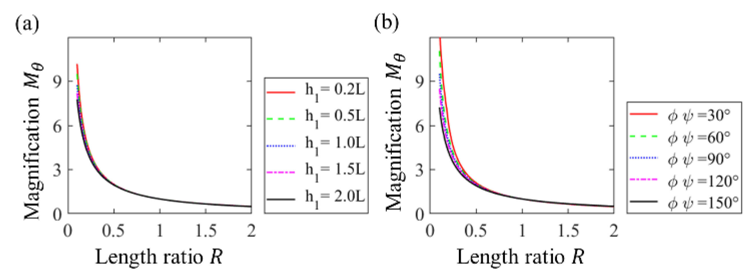
3.1. Angle and Torque Magnification of a Single Four-Bar Linkage Structure

With a single four-bar linkage structure defined as the basic topological element of the model adaptive gripper finger, its kinematics and the relationship between the angle and torque magnifications are investigated in this section.

As illustrated in Figure 6a, a single four-bar linkage structure was attached to a triangular fingertip. Here, L is the reference length of the linkage structure, $h_1$ is the length of the input linkage, and $h_2$ is the length of the output linkage. The length ratio between $h_2$ and $h_1$ is defined as R. The symbol for the initial input angle of the linkage is φ, whereas the angle $\psi$ is used to represent the initial output angle. The deviations or changes from φ and $\psi$’s initial values are denoted as ${\delta }_1$ and ${\delta }_2$, respectively. The relationship between the input angle change ${\delta }_1$ and output angle change ${\delta }_2$ is denoted as the angle magnification and can be obtained using Equation (11).

This angle magnification is sensitive to the linkage design parameters. For instance, as shown in Figure 7, the angle magnification of a single four-bar linkage finger is plotted with different length ratios R ranging from 0.1 (leftmost curve) to 10 (bottommost curve) for several h₁ values. Each curve in the plot is terminated with an “x” mark to indicate the kinematic limit before reaching the singularity. When $h_1=h_2$, that is, R = 1, the four-bar linkage becomes a parallelogram. As such, a one-to-one mapping between the input angle ${\delta }_1$ and output angle ${\delta }_2$ occurs. Thus, a greater angle magnification between ${\delta }_1$ and ${\delta }_2$ can be achieved with a minimum R. On the other hand, if $h_2$ is larger than $h_1$, that is, R is greater than 1, a smaller angle magnification is obtained.

The ${\delta }_1$ to ${\delta }_2$ ratio also depended on the φ and $\psi$’s initial values. The illustrative examples in Figure 8 show that with $h_1$ = 0.5L, significant shrinkage in the range of motion occurs when the same initial angle value, ranging from 30° to 150°, is assigned to both φ and $\psi$. In addition, setting the angle magnification M_θ equal to ${\delta }_2/{\delta }_1$, as illustrated in Figure 9, the M_θ value decreases exponentially with an increase in the length ratio R. By changing the ratio R from 0.2 to 2, the angle magnification M_θ between different $h_1$ does not change significantly, as shown in Figure 9a. Furthermore, with the change in the initial angle φ and $\psi$ in Figure 9b, the angle magnification M_θ shows a similar trend.

We define torque magnification M_T as the ratio of the output torque provided by the fingertip to the input torque, which is applied by actuators at r₂ with respect to P₁ of the single four-bar linkage. We observed that M_T also deviates from linearity when measured with respect to the input angle ${\delta }_1$, at length ratios ranging between 0.2 and 2.0, as illustrated in Figure 10. The results show that with an increase in length $h_1$, the torque magnification increases with a fixed length ratio R smaller than one. However, as in the angle-magnification case, the range of motion becomes smaller when R is greater than one.

3.2. Range of Motion for Double-Section Structures

An adaptive finger model composed of two identical four-bar linkage structures, as illustrated in Figure 6b, is investigated in this section. Keeping L as the reference linkage length of the second linkage structure, $h_1$ as the input linkage length, $h_2$ as the output linkage length, and the length ratio between $h_2$ and $h_1$ as R, this adaptive finger also possesses the same notation for the initial angular values φ of the input and $\psi$ of the output, and the corresponding angle increments ${\delta }_1$ and ${\delta }_2$. Due to the identical structure of each four-bar linkage in this adaptive finger, the same value for each parameter is applied to each linkage structure. To determine the effect on the range of motion for the linkage parameters, scatter 2-D plots are presented in Figure 11 for the case of $h_1=$ 1.0L, with length ratio R set at 0.5, 1.0, and 1.2 in (a) to (c) to show the fingertip’s positions. For the R = 1.0 case, one can observe that the ratio between the output and input angles is maintained regardless of the ${\theta }_5$ value changed. It can be seen in the scatter plots that larger ranges of motion can be achieved when R < 1 in the double four-bar linkage robotic finger.

The values of the double four-bar linkage adaptive finger’s initial angles φ and $\psi$ can slightly affect the fingertip’s positions in the X–Y coordinates, but have a large influence on the input angle range, as well as the relationship between the input and output angles. As shown in Figure 12, for $h_1=1.0L$ and R = 0.5, with initial angles φ and $\psi$ both set to 45°, 90°, and 135°, the initial angle value alters the relationship between the input and output angles in the adaptive finger. Consequently, larger R, φ$,$ and $\psi$ values lead to a significant decrease in the range of motion of the robotic finger.

3.3. Range of Motion for Triple-Section Structures

Similar to the double four-bar linkage adaptive finger, the adaptive robotic finger shown in Figure 5c was constructed with three identical four-bar linkage structures. With the same structure as those defined in the single and double four-bar linkage cases, scatter plots showing the fingertip’s X–Y positions are presented in Figure 13, for cases where $h_1=1.0L$ with length ratio R set at 0.5, 1.0, and 1.2. The correlation between the input angle ${\delta }_1$ by the actuator and the output angle ${\delta }_2$ of the fingertip is also shown in Figure 13. In addition to reaching the same conclusions as for the double four-bar linkage cases, a larger range of motion was observed for the triple four-bar linkage structures. The effects of the initial angles φ and $\psi$ for the triple four-bar linkage structures are illustrated in Figure 14 for $h_1=1.0L$ and $R=0.5$ with initial angles φ and $\psi$ both set to 45°, 90°, and 135°, respectively. The same motion behavior between the input and output angles as in the double four-bar linkage structure was observed in this triple four-bar linkage structure, in which the initial angle values φ and $\psi$ significantly affected the finger’s range of input angles.

4. Mechanism Adaptive Results

To validate the aforementioned kinematic analyses, a prototype design of an adaptive robotic gripper that can be used in various environments was presented and investigated in this section. In contrast to the design of a general-purpose robot gripper, the goal of the gripper is to assist industrial, commercial, and even home applications. To achieve this goal, the gripper was designed with maximum flexibility and high adaptivity for grasping objects, similar to a human hand. When humans attempt to grasp an irregular object, their fingers naturally cover the object according to the length of the object’s surface. To achieve this humanoid grasping motion, the proposed adaptive robotic finger must be composed of several four-bar linkage structures to provide extra degrees of freedom for grasping.

In addition to the finger linkage structures, the number of fingers is another key engineering design factor for robotic grippers. Evidentially, more fingers naturally offer a more stable gripping when grasping irregular objects. Interestingly, most industrial robotic grippers are designed with two parallel rigid fingers. However, if the object’s shape is irregular or asymmetric, gripper designs with more than two fingers are of a natural choice, as evidenced by S. B. Backus and A. M. Dollar [19], to achieve stable grasping operations.

The effects of the linkage parameters on the range of motion for double-section and triple-section structures are listed in

Table 1. Range of motion for different linkage parameters.

Range of Motion at End Point (mm2)		Double-Section Structures			Triple-Section Structures
		h1 = 0.5	h1 = 1.0	h1 = 1.5	h1 = 0.5	h1 = 1.0	h1 = 1.5
R = 0.5	φ & $\psi$ = 45°	249.0	234.2	252.7	652.8	661.0	667.9
	φ & $\psi$ = 90°	238.5	233.2	248.2	535.7	630.3	663.3
	φ & $\psi$ = 135°	75.1	229.6	198.2	161.6	538.8	484.5
R = 1.0	φ & $\psi$ = 45°	212.1	215.3	214.0	199.7	195.9	195.0
	φ & $\psi$ = 90°	105.3	95.1	219.8	160.6	159.2	158.9
	φ & $\psi$ = 135°	19.6	14.7	19.4	28.4	26.0	26.2
R = 1.2	φ & $\psi$ = 45°	54.1	37.2	33.5	64.0	51.4	40.5
	φ & $\psi$ = 90°	20.2	10.3	11.5	17.5	14.0	12.6
	φ & $\psi$ = 135°	4.2	2.9	2.0	3.4	2.2	1.9

. First, we denote the effect of the length ratio R between $h_2$ and $h_1$. With the same parameters, a larger R was found to decrease the range of motion for both the double- and triple-section structures. Second, with the change in initial angle φ and $\psi$, a larger initial angle slightly decreases the range of motion at the endpoint. However, it obviously decreases the range of the input angle ${\delta }_1$ as illustrated in Figure 12 and Figure 14. Third, the length of $h_1$ can slightly change the range of motion when different length ratios R are applied. When R is smaller than 1, a greater $h_1$ value slightly increases the range of motion. However, when R is greater than 1, a larger $h_1$ can decrease the range of motion. Finally, by comparing the double- and triple-section structures, the triple-section structures were found to be able to achieve a larger motion range in most cases.

In this study, an adaptive gripper with three identical fingers was developed. Each finger of the gripper utilized three four-bar linkage structures to mimic the fingers of the human hand with MCP, PIP, and DIP joints. The parameters of the gripper finger structure are $L=30 \mathrm{mm}, h_1=0.8, R=0.5, \mathrm{and} =\psi =60°$. We then analyzed its kinematics using the previously presented analytical model, as discussed in the previous sections. The gripper specifications are listed in

Table 2. Specifications of the gripper.

Operation Range	Speed	Force	Load	Weight
160 mm	100 mm/s	50 N	5 kg	1.5 kg

. The range of motion of the gripper is illustrated in the scatter plot in Figure 15 to show the positions that the adaptive robotic finger can reach.

The gripper can change its shape along the surface of the object, as illustrated in the simulations (top) and experiments (bottom), as shown in Figure 16. Using the cylindrical object in Figure 16a and different-sized boxes in Figure 16b–d as the target objects to be grasped, the adaptive feature of the gripper finger to the object’s surface was demonstrated. As the orientation of each of the three adaptive fingers of the gripper can be controlled independently, high spatial adaptivity was also observed when grasping cylindrical, spherical, and irregularly shaped objects, as shown in the photos in Figure 17.

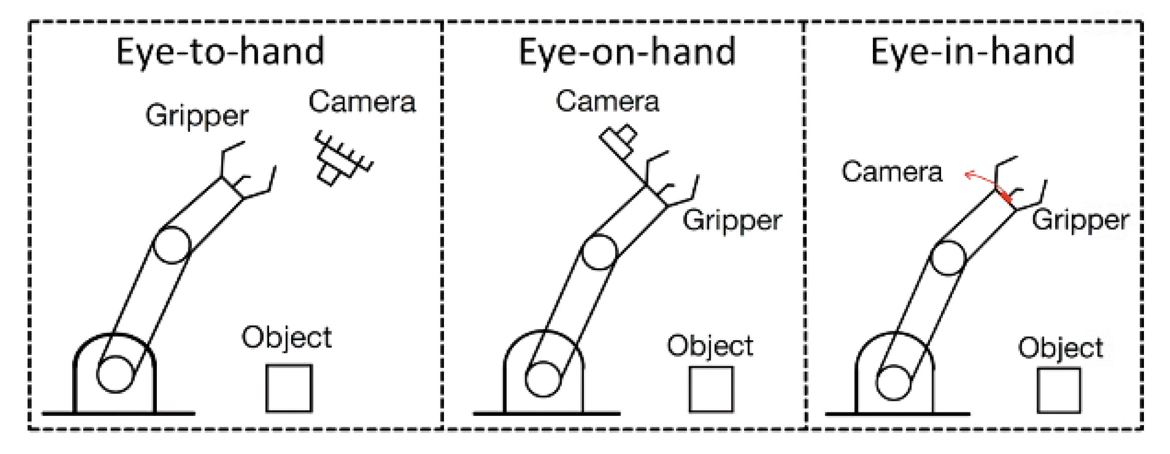
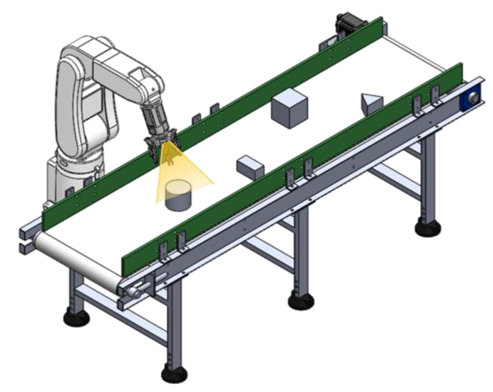
5. Visual Adaption by Eye-in-Hand System

In addition to the mechanical-adaptive feature, a vision-adaptive function was encapsulated with the gripper. To automatically grasp objects in industrial applications or to serve as a helping robot for disabled people, a vision-adaptive feature is an important factor for a universal-purpose robot gripper. Owning to the processor’s speed limit, the Raspberry PI computer embedded in the gripper cannot process and execute a complex object recognize algorithm. Therefore, a simple object recognition algorithm to allow the gripper with a robotic manipulator to conduct pick-and-place task was developed, implemented, and examined by using the platform as shown in Figure 18, where the target objects were carried by a constant-speed conveyor belt. The gripper is equipped with an eye-in-hand camera to capture objects on the conveyor and pick up objects of any shape with its mechanical-adaptive feature. Regardless of the object, the gripper can automatically change its profile and orientation between the fingers to conduct adaptive grasping operations.

The information of the target object was acquired and analyzed from the eye-in-hand vision system, which was later used to control the movement of the manipulator. Mathematically, the location, orientation, and shape of a target object in world coordinates are required parameters to complete the transformation matrix from camera coordinates to object coordinates. To find, identify, and even realize the shape and profile of a target object, two image processing methods were used: color space processing and contour processing of the target, respectively. The image processing method and visual servoing flowchart are depicted in Figure 19 to outline the grasping operation for the gripper to achieve the goal of automated object tracking and grasping. When the gripper finds the target, it sends commands to move the manipulator to locate the target and try to grasp it. If the target is moving, the camera system determines the velocity and then tries to follow the moving object. To calculate the position of the target, the translation from the image coordinate frame to the robot coordinate frame is presented in the following context.

5.1. Color Model for Object Image Processing

To demonstrate the visual adaption feature of the model system, objects were placed arbitrarily on a moving green-color conveyer belt without physically overlapping and colliding with each other. As image processing can be easily inferred by ambient light, processing the captured image in the form of a hue-saturation-value (HSV) dataset was used in this study instead of the commonly used red-green-blue (RGB) format. It subtracted unnecessary image areas in the captured image and printed out the image of the target object.

HSV image data are advantageous because they are not sensitive to environmental light, whereas RGB image data are significantly affected by brightness. As illustrated in Figure 20, the captured RGB image processed by the HSV color model removes the influence of ambient brightness, where the green region represents the conveyor belt, the brown region represents the frame of the conveyor, and the pink region is the target. From this processed image, one can easily find the target region and separate it from the other regions.

5.2. Finding Object’s Location, Orientation and Shape

After identifying the target object in the captured image, the Douglas–Peucker [20] algorithm was used to find the vertices of the contour of the object. Using the Douglas–Peucker algorithm, a polyline composed of numerous points can be simplified into a few vertices. As an example, as shown in Figure 21a, the original polyline contains eight points that start from point A to point B. Then, in Figure 21b, when drawing line a, which links from point A to point B, we can find point P₁, which is the furthest point to line a. If the distance b between line a and P₁ is larger than the threshold value set for the Douglas–Peucker algorithm, P₁ is one of the vertices in this polyline, and the polyline can be separated into two. Using the same rule, P₂ and P₃ are shown in Figure 21c,d, respectively. Finally, we obtained a new polyline constructed with five points and three vertices, as shown in Figure 21e.

The shape of the target object is determined by calculating the number of vertices. Utilizing the locations of these vertices, the orientation and centroid location of the target object can be determined by using trigonometric functions. As illustrated, examples as shown in Figure 22, the object contour and corresponding centroid location (marked by red dots) were found by using the Douglas–Peucker algorithm. With the found contour, the objects were further classified into triangular, rectangular, or circular shapes according to the number of edge points, which is the number of vertices of the contour of the object. When three edges were detected, the target was determined as a triangle. If the number of vertices of a target exceeded the threshold, set to 10 in this case, it was considered as a circular object in this study.

As indicated in the left portion of Figure 22, α, which is defined as the angle between the moving axis of the underlying conveyer belt and the edge of the object, can be calculated to provide orientation information of the target object with respect to the fixed moving direction of the conveyor belt. With the Douglas–Peucker algorithm applied to the captured image from the eye-in-hand camera, the adaptive gripper can find each edge point’s location, as well as the orientation and location of the target object by calculating the edge points. With the shape, location, and orientation data, the gripper can easily locate the target object and adjust its finger orientations to match the object in grasping operations. As the camera coordinates and gripper coordinates coincided, calibration between the coordinates was not necessary, which facilitated the control practice of the gripper to grasp targets in engineering applications. As shown on the right side of Figure 22, the target object should have a triangular or circular shape, and a three-finger mode is engaged, in which each of the gripper fingers is oriented 120° with each other for an equilateral triangle or a circular object. If the triangle-shaped object is not an equilateral triangle, the three-finger mode is still employed, but the orientation of each gripper finger is automatically adjusted accordingly. On the other hand, if the object is determined to be square or rectangular in shape, a two-finger mode is engaged, in which two of the three fingers are oriented to be adjacent to each other, and the other one is oriented 180° from the two fingers, as illustrated in the top-right picture in Figure 22.

5.3. Motion Planning

Once the image is captured by the eye-in-hand camera of the gripper, the camera coordinates must be converted into global coordinates for path planning to allow the gripper to accurately track the moving object.

The coordinate frames for a six-degrees-of-freedom robot (Universal Robot 5 in this case) and eye-in-hand robotic gripper system are defined as follows:

• Manipulator base coordinate frame $\left\{\left.B\right\}\right.$;
• Tool (end-effector) coordinate frame $\left\{\left.T\right\}\right.$;
• Eye-in-hand camera coordinate frame $\left\{\left.C\right\}\right.$;
• Object coordinate frame $\left\{\left.O\right\}\right.$, which is the surface of the object.

For simplicity, the eye-in-hand camera was installed in the center of the palm; therefore, the camera frame was the same as the gripper frame, which was not particularly defined in this study. The relationship between the aforementioned frames is illustrated in Figure 23, and the calibration matrix of this system is given by:

$$M_B^T\left(New\right)M_T^O=M_B^T\left(Previous\right)M_T^C{M}_C^O$$

(12)

Here, $M_B^T\left(Previous\right)$ is the transformation matrix for the previous position and $M_B^T\left(New\right)$ is the transformation matrix of the position to which the gripper is expected to move. Thus, the gripper can use inverse kinematics to move toward the target posture. In Equation (12), $M_T^O$, $M_T^C$, and $M_C^O$ are transformation matrices, as shown in Figure 24, and are expressed as:

$$M_T^O=\left[\begin{array}{cccc}1& 0& 0& 0\\ 0& 1& 0& 0\\ 0& 0& 1& t\\ 0& 0& 0& 1\end{array}\right]$$

(13)

$$M_T^C=\left[\begin{array}{cccc}1& 0& 0& 0\\ 0& 1& 0& 0\\ 0& 0& 1& d\\ 0& 0& 0& 1\end{array}\right], \mathrm{and}$$

(14)

$$M_C^O=\left[\begin{array}{cccc}\cos (R_Z)& -\sin (R_Z)& 0& \frac{\mathsf{\Delta }u\times z}{\alpha }\\ \sin (R_Z)& \cos (R_Z)& 0& \frac{\mathsf{\Delta }v\times z}{\beta }\\ 0& 0& 1& z^{\prime }\\ 0& 0& 0& 1\end{array}\right],$$

(15)

respectively. The $M_T^O$ is the transformation matrix from object coordinates to tool coordinates, t is the distance between the tool frame and the object frame, whereas the $M_T^C$ is the transformation matrix from the camera coordinates to the tool coordinates, and d is the distance between the tool frame and the camera frame. Last but not least, the $M_C^O$ is the transformation matrix from object coordinates to camera coordinates, in which expression $R_Z$ is the orientation of the target object, $z$ is the distance between the camera frame and the object frame, $z^{\prime }$ is the distance between the expected grabbing position and the object frame, $\mathsf{\Delta }u$ and $\mathsf{\Delta }v$ are the pixels between the center of the target object point and the center of the image, and $\alpha$ and $\beta$ are the calibrate parameters in the intrinsic matrices of the camera.

5.3.1. Conversion of Image Coordinates

To locate the target position, intrinsic and extrinsic matrices are utilized to convert the image coordinates to world coordinates, so that the real-world distance corresponding to each pixel can be determined. This conversion is illustrated in Figure 25. The conversion between the camera image coordinates ${\left[\begin{array}{ccc}u& v& w\end{array}\right]}^T$ and global coordinates ${\left[\begin{array}{ccc}X& Y& Z\end{array}\right]}^T$ can be expressed as:

$$\left[\begin{array}{c}u\\ v\\ w\end{array}\right]=K\left[R | t\right]\left[\begin{array}{c}\begin{array}{c}X\\ Y\end{array}\\ \begin{array}{c}Z\\ 1\end{array}\end{array}\right]=\left[\begin{array}{ccc}\alpha & s& u_0\\ 0& \beta & v_0\\ 0& 0& 1\end{array}\right]\left[\begin{array}{cccc}{r}_{11}& r_{12}& r_{13}& t_x\\ r_{21}& r_{22}& r_{23}& t_y\\ r_{31}& r_{32}& r_{33}& t_z\end{array}\right]\left[\begin{array}{c}\begin{array}{c}X\\ Y\end{array}\\ \begin{array}{c}Z\\ 1\end{array}\end{array}\right]$$

(16)

where the multiplication of $K$ and $\left[R | t\right]$ forms a projection matrix. This projection matrix can be split into two matrices: intrinsic parameter matrix K and extrinsic parameter matrix $\left[R | t\right]$. In Equation (16), $u_0$ and $v_0$ represent the pixels of the image plane center corresponding to the X- and Y-axes. Ideally, if the camera has a resolution of 800 × 600 pixels, $u_0$ is 400 pixels, and $v_0$ is 300 pixels. The $\alpha$, $\beta$, and $s$ are the calibration parameters in the intrinsic matrices of the camera, where $\alpha$ and $\beta$ are the focal lengths of the camera in the X- and Y-axes, respectively. Finally, the $s$ represents the distortion correction factor if the X- and Y-axes are not perpendicular to each other. By contrast, the extrinsic parameter matrix $\left[R | t\right]$ is the transformation between the world coordinate system and the camera coordinate system, which is the transformation matrix $M_B^C$ that converts the base frame into a camera frame.

There is no available intrinsic matrix information on the Raspberry PI3’s 2-D camera data sheet. To determine the intrinsic parameters of the camera that are not commercially available or offered by the Raspberry PI3’s 2-D camera used in this study, we adopted the method established by Zhang [21] to determine the intrinsic matrix parameters by using a checkerboard to constrain intersection points on the same plane. Using this method, depth information Z can be ignored in the projection matrix, therefore, Equation (16) can be rewritten as follows:

$$\left[\begin{array}{c}u\\ v\\ 1\end{array}\right]=\left[\begin{array}{ccc}\alpha & s& u_0\\ 0& \beta & v_0\\ 0& 0& 1\end{array}\right]\left[\begin{array}{ccc}{r}_{11}& r_{12}& t_x\\ r_{21}& r_{22}& t_y\\ r_{31}& r_{32}& t_z\end{array}\right]\left[\begin{array}{c}X\\ Y\\ 1\end{array}\right]=\left[\begin{array}{ccc}{h}_1& h_2& h_3\end{array}\right]\left[\begin{array}{c}X\\ Y\\ 1\end{array}\right]=H\left[\begin{array}{c}X\\ Y\\ 1\end{array}\right]$$

(17)

Here, the H matrix is a 3-by-3 matrix derived by multiplying the intrinsic matrix with the modified extrinsic matrix. Using the checkerboard, as suggested by Zhang [21], the intrinsic parameters can be determined by decomposing the H matrix. As the modified extrinsic matrix is not composed of the rotation matrix and translation vector, it cannot be directly decomposed using QR decomposition. To decompose the H matrix, the two constraints $r_1$ and $r_2$ possess orthogonal properties in the form:

$$\left[\begin{array}{ccc}{h}_1& h_2& h_3\end{array}\right]=K\left[\begin{array}{ccc}{r}_1& r_2& t\end{array}\right]$$

(18)

where $r_1=K^{-1}{h}_1 \mathrm{and} r_2=K^{-1}{h}_2$. As $r_1$ and $r_2$ are orthogonal, therefore:

$$r_1{r}_2=0\Rightarrow h_1^T{K}^{-T}{K}^{-1}{h}_1=0$$

(19)

$$\left|r_1\right|=\left|r_2\right|=1\Rightarrow h_1^T{K}^{-T}{K}^{-1}{h}_1-h_2^T{K}^{-T}{K}^{-1}{h}_2=0$$

(20)

Matrix B is defined as the inverse and transpose of the intrinsic matrix multiplied by the inverse of the intrinsic matrix. That is, $B=K^{-T}{K}^{-1}$. This B matrix is in fact a Hermite matrix, which can be decomposed into the definiteness of a matrix multiplied by the Hermitian transpose matrix to determine the intrinsic parameters. As conversion errors exist because of manufacturing and assembling imperfections, it is necessary to find the corresponding intrinsic matrix to minimize the errors, and make the $r_1$ and $r_2$ vectors orthogonal.

Until now, we have not considered lens distortion of the camera. The lens distortion parameter matrix K can be calculated using the OpenCV image processing library to find the ideal pixel of the image acting as the target object center. We define (u, v) as the ideal pixel image coordinates and ($\tilde{u}$, $\tilde{v}$) as the corresponding real observed image coordinates, where (x, y) and ($\tilde{x}$, $\tilde{y}$) are their world coordinates, respectively. Owing to the pinhole camera model, the ideal position versus the distance of the target equals the pixel versus the focal length. That is, we can express this relationship as:

u (pixel position):f (focal length) = x (global position) and z (target distance)

(21)

Assume ${\tilde{x}}^{\prime }=\frac{\tilde{x}}{z} ,{\tilde{y}}^{\prime }=\frac{\tilde{y}}{z} ,x^{\prime }=\frac{x}{z} ,\mathrm{and} y^{\prime }=\frac{y}{z}$, where z is the height of the target object, as expressed in Equation (25). ${\tilde{x}}^{\prime }$ and ${\tilde{y}}^{\prime }$ can then be rewritten as:

$${\tilde{x}}^{\prime }=\frac{\tilde{u}-u_0}{\alpha }, {\tilde{y}}^{\prime }=\frac{\tilde{v}-v_0}{\beta }.$$

(22)

Assuming that $r^2=\left({{\tilde{x}}^{\prime }}^2+{{\tilde{y}}^{\prime }}^2\right)$, the ideal world coordinates are given by:

$$\begin{gathered} x^{\prime }={\tilde{x}}^{\prime }\left(1+k_1{r}^2+k_2{r}^4+k_3{r}^6\right)+2P_1{\tilde{x}}^{\prime }{\tilde{y}}^{\prime }+P_2\left(r^2+2{{\tilde{x}}^{\prime }}^2\right) \\ {y}^{\prime }={\tilde{y}}^{\prime }\left(1+k_1{r}^2+k_2{r}^4+k_3{r}^6\right)+2P_2{\tilde{x}}^{\prime }{\tilde{y}}^{\prime }+P_1\left(r^2+2{{\tilde{y}}^{\prime }}^2\right) \end{gathered}$$

(23)

where k₁, k₂, k₃, P₁, and P₂ are distortion parameters. Finally, the ideal pixel (u, v) can be expressed as:

$$u=\alpha x^{\prime }+u_0, v=\beta y^{\prime }+v_0$$

(24)

5.3.2. Determine the Height of the Target Object

As the camera in the eye-in-hand gripper module is a 2-D camera, the height r of the manipulator, as shown in Figure 26, can only be obtained through the manipulator encoder. From the projection matrix, the z information is defined from the camera frame to the surface of the target object, which can be expressed as:

$$z=r-h-c$$

(25)

where parameter c is the height of the conveyor. Different objects have different heights; therefore, the first step in the gripping action is to determine the height of the target object by moving the manipulator. The relationship between the distance moved by the manipulator and h information is given by:

$$h=\frac{d\ast \alpha }{u_2-u_1} \mathrm{or} h=\frac{d\ast \beta }{v_2-v_1},$$

(26)

where $\alpha$ and $\beta$ are the camera’s intrinsic parameters, d is the distance moved by the manipulator, $u_1$ and $v_1$ are the target image pixel center coordinates before the manipulator is moved, and $u_2$ and $v_2$ are the target image pixel center coordinates after the manipulator is moved. After these parameters were considered, the height of the target object could be calculated.

5.3.3. Image-Based Visual Servo Control

In this study, the target object was placed on a conveyor belt traveling at a constant speed $V_{conveyor}$. The speed of the conveyor belt can be pre-set by the user or be calculated by the target’s movement in serval frames as:

$$V_{conveyor}=\frac{\sqrt{{\left({\tilde{x}}_2-{\tilde{x}}_1\right)}^2+{\left({\tilde{y}}_2-{\tilde{y}}_1\right)}^2}}{\Delta T_{frame}}$$

(27)

where $\tilde{x}$ and $\tilde{y}$ are the real position of the object, subscripts 1 and 2 indicate two incremental time indexes, and $\Delta T_{frame}$ is the period of the camera’s update rate. It was observed that once the eye-in-hand gripper system received a command to move the manipulator to a desired position, owing to the required computation overhead time, the target had already moved to a new position. Therefore, it is imperative to calculate the movement speed of the conveyor and account for its motion when moving the manipulator. However, the estimation of the target object’s moving speed is required for the gripper to successfully track and grasp the object. Mathematically, the area under the velocity-time diagram is equivalent to the distance between the gripper (camera) and the object centers, the function of which is given by the following equation:

$$V_t=\left(V_{t-1}+aT\right)\pm \sqrt{a^2{T}^2+2a\left(V_{t-1}T-X\right)}$$

(28)

where $V_t$ is the output speed, $V_{t-1}$ is the speed of the previous iteration of the manipulator, $T$ is the time of each iteration, $a$ is the acceleration, and $X$ is the distance between the gripper and the object centers. To determine the output speed, the sign of the acceleration is first determined. The acceleration is positive when $X$ is greater than $V_{t-1}\times T$. Otherwise, it is negative. However, the value in the square root must be positive. If $a^2{T}^2+2a\left(V_{t-1}T-X\right)$ is less than zero, then $X$ is too large under this acceleration. In this case, $X$ must be modified to satisfy these conditions. As the speed of the conveyor is constant, the speed of the manipulator can be similar in each iteration. This speed can be assumed to be the speed of the conveyor so that the eye-in-hand gripper system can compensate for the object’s motion at the last iteration because of the known speed of the conveyor. Therefore, the total speed is given by:

$$V_{total}=V_t+V_{conveyor}$$

(29)

6. Visual Adaption Results

The purpose of the vision adaptive feature is to grasp target objects adaptively according to their shape and motion. To achieve this, the experimental setup was divided into three steps. The first step was to determine the shape and orientation of the target object. The second step was to find the positional information, which was converted from image pixels to real-world coordinates so that the error of the conversion at an unknown target object height can be determined. In the third step, the speed of the target was obtained, and the manipulator was set to chase the target at a constant speed.

The performance of the visual adaptivity is listed in

Table 3. Height measurement of target objects.

Height Measurement	Average Height of Calculation (m)	Average Height of Measurement (m)	Standard Deviation (m)	Error Rate (%)
Square	0.049	0.050	0.004	1.71%
Circle	0.053	0.051	0.001	5.16%
Rectangle	0.024	0.024	0.002	1.08%

for three different target objects, namely, square, circle, and rectangle objects, respectively. The maximum standard deviation of measurements in sensing an object’s height was approximately 4 mm, which is in reasonable range limited by a commercially available depth camera. For the Intel Realsense camera used in this study, its depth accuracy is 2.5 mm to 5 mm at 1 m distance from object to camera, which reconfirms the mentioned 4 mm standard deviation is engineering reasonable. Certainly, should a better depth camera be used, this number can be further improved.

Once a target’s height was measured, the smart gripper started to locate the target and follow its movement using its eye-in-hand visual servoing function.

Table 4. Visual servoing results at different conveyor speeds.

Conveyor Moving Speed		Speed 20 mm/s	Speed 40 mm/s	Speed 60 mm/s	Speed 70 mm/s
Square	Moving Distance (m)	0.133	0.245	0.326	0.430
	Standard Deviation (m)	0.008	0.020	0.020	0.034
	Success Rate (%)	100%	100%	100%	70%
Circle	Moving Distance (m)	0.132	0.247	0.315	0.429
	Standard Deviation (m)	0.007	0.013	0.025	0.022
	Success Rate (%)	100%	100%	100%	85%
Rectangle	Moving Distance (m)	0.131	0.244	0.315	0.411
	Standard Deviation (m)	0.008	0.017	0.021	0.021
	Success Rate (%)	100%	100%	100%	100%

shows results of the success rate for the gripper to perform the visual servoing function at different speeds of the conveyor. The results show the maximum conveyor speed that can be chased up by the gripper was approximately 70 mm/s. It was also observed that success rates when speed was below 70 mm/s remained at 100% for the different targets and rapidly decreased at 70 mm/s. Constrained by the total length of the conveyor belt being 70 cm and its effective length being 50 cm to prevent objects dropping at its two edges, the maximum speed that can be tested was then limited.

Figure 27 shows the real-time velocity of the manipulator’s tool center point (TCP) when the gripper attempts to grasp a moving object. The velocity profile was divided into four regions. In region I, the gripper calculates the moving speed and shape of the target. In Region II, the gripper sends the target information to the controller to track the target. In region III, the gripper speed was set identical to that of the moving target. Subsequently, the gripper’s TCP center starts to align with the moving target’s center. During the finding and tracking process, the gripper started to change the angle between its fingers to ensure a proper grasping posture. Finally, in region IV, the robotic arm prepares to execute a grasp mission while waiting for its speed to be identical to that of the target. As shown in Figure 27, the distance moved by the object can be obtained by multiplying the speed of the conveyor with time. The distance that the manipulator moves is determined by the manipulator’s feedback. When the distance between the robot and the object is close enough to grasp, and when the object is directly below the eye-in-hand gripper module, the object can be grasped by the robotic gripper.

Consequently, the gripper can grasp different types of objects of any shape in any orientation, regardless of whether the object is moving or stationary. Figure 28 shows the vision tracking results for two different objects moving on a conveyor. With the vision adaptive function, the general adaptive gripper can not only grasp irregular objects but also moving targets.

7. Conclusions

In this study, a new type of adaptive gripper was proposed, analyzed, and validated through analytical and experimental approaches. Each finger in the proposed adaptive gripper comprised a series of four-bar linkage structures, offering compliance as well as adaptability when adapting to an object’s surface with redundant degrees of freedom in the model gripper. The proposed adaptive robotic gripper consisted of three identical fingers, each of which was composed of three four-bar linkage structures that can be independently controlled to change their orientations. With its adaptive features and three-finger structure, the proposed adaptive gripper demonstrated the feasibility of stable and reliable grasping of objects of various shapes.

This study also implemented an efficient method for camera recognition, positioning, and tracking control using an eye-in-hand robotic configuration. The main advantages of eye-in-hand configuration include occlusion avoidance, intuitive teleoperation, imaging at various angles, easier calibration, and high accuracy. Furthermore, the proposed eye-in-hand robotic gripper featured a modular design and did not require an extra computer, power, or Ethernet cables to communicate with the Raspberry PI3 controller and robotic articulator such as UR5. All these features make it convenient for real-life application scenarios. In addition, an object tracking system was established to allow the underlying robotic manipulator to carry the proposed gripper to track objects on a constant-speed conveyor.

The first contribution of this research was the establishment of a mathematical kinematic model of four-bar linkages in the design of adaptive fingers. Using this analytical model, the position, velocity, and torque transmission of the adaptive robotic finger can be derived. Second, a prototypical adaptive three-finger robotic gripper designed using the derived analytical model was developed, and its specifications were validated through quantitative analytical predictions and qualitative experimental observations. Finally, an eye-in-hand gripper prototype was developed by using an eye-in-hand sensor, allowing the gripper to easily track target objects and execute appropriate grasping actions. By using a general RGB camera with the depth calculation feature, it provided an approximate 4 mm standard deviation in depth error, which was similar to the depth accuracy of an Intel Realsense RGB-D camera. On the other hand, the gripper achieved a 100% grasping success rate when the conveyor speed was lower than 70 mm/s with different objects.

References

1. Jin, J.; Zhang, W.; Sun, Z.; Chen, Q. LISA Hand: Indirect self-adaptive robotic hand for robust grasping and simplicity. In Proceedings of the 2012 IEEE International Conference on Robotics and Biomimetics (ROBIO), Guangzhou, China, 11–14 December 2012; pp. 2393–2398. [Google Scholar]
2. Kappassov, Z.; Khassanov, Y.; Saudabayev, A.; Shintemirov, A.; Varol, H.A. Semi-anthropomorphic 3D printed multigrasp hand for industrial and service robots. In Proceedings of the 2013 IEEE International Conference on Mechatronics and Automation, Takamatsu, Japan, 4–7 August 2013; pp. 1697–1702. [Google Scholar]
3. Li, G.; Zhang, W. Study on coupled and self-adaptive finger for robot hand with parallel rack and belt mechanisms. In Proceedings of the 2010 IEEE International Conference on Robotics and Biomimetics, Tianjin, China, 14–18 December 2010; pp. 1110–1115. [Google Scholar]
4. Telegenov, K.; Tlegenov, Y.; Shintemirov, A. A low-cost open-source 3-d-printed three-finger gripper platform for research and educational purposes. IEEE Access 2015, 3, 638–647. [Google Scholar] [CrossRef]
5. Birglen, L.; Gosselin, C.M. Geometric design of three-phalanx underactuated fingers. J. Mech. Des. 2006, 128, 356–364. [Google Scholar] [CrossRef]
6. Birglen, L.; Gosselin, C.M. Kinetostatic analysis of underactuated fingers. IEEE Trans. Robot. Autom. 2004, 20, 211–221. [Google Scholar] [CrossRef]
7. Birglen, L.; Gosselin, C.M. Force analysis of connected differential mechanisms: Application to grasping. Int. J. Robot. Res. 2006, 25, 1033–1046. [Google Scholar] [CrossRef]
8. Cheng, L.-W.; Chang, J.-Y. Design of a Multiple Degrees of Freedom Robotic Gripper for Adaptive Compliant Actuation. In Proceedings of the 2018 International Conference on System Science and Engineering (ICSSE), New Taipei City, Taiwan, 28–30 June 2018; pp. 1–6. [Google Scholar]
9. Barth, R.; Hemming, J.; van Henten, E.J. Design of an eye-in-hand sensing and servo control framework for harvesting robotics in dense vegetation. Biosyst. Eng. 2016, 146, 71–84. [Google Scholar] [CrossRef] [Green Version]
10. Chang, W.-C. Robotic assembly of smartphone back shells with eye-in-hand visual servoing. Robot. Comput.-Integr. Manuf. 2018, 50, 102–113. [Google Scholar] [CrossRef]
11. Pomares, J.; Perea, I.; García, G.J.; Jara, C.A.; Corrales, J.A.; Torres, F. A multi-sensorial hybrid control for robotic manipulation in human-robot workspaces. Sensors 2011, 11, 9839–9862. [Google Scholar] [CrossRef] [PubMed]
12. Cigliano, P.; Lippiello, V.; Ruggiero, F.; Siciliano, B. Robotic ball catching with an eye-in-hand single-camera system. IEEE Trans. Control. Syst. Technol. 2015, 23, 1657–1671. [Google Scholar] [CrossRef] [Green Version]
13. Shaw, J.; Chi, W.-L. Automatic classification of moving objects on an unknown speed production line with an eye-in-hand robot manipulator. J. Mar. Sci. Technol. 2018, 26, 10. [Google Scholar]
14. Yu, S.; Lee, J.; Park, B.; Kim, K. Design of a gripper system for tendon-driven telemanipulators considering semi-automatic spring mechanism and eye-in-hand camera system. J. Mech. Sci. Technol. 2017, 31, 1437–1446. [Google Scholar] [CrossRef]
15. Wang, H.; Guo, D.; Xu, H.; Chen, W.; Liu, T.; Leang, K.K. Eye-in-hand tracking control of a free-floating space manipulator. IEEE Trans. Aerosp. Electron. Syst. 2017, 53, 1855–1865. [Google Scholar] [CrossRef]
16. Florence, P.R.; Manuelli, L.; Tedrake, R. Dense object nets: Learning dense visual object descriptors by and for robotic manipulation. arXiv 2018, arXiv:1806.08756. [Google Scholar]
17. Shih, C.-L.; Lee, Y. A simple robotic eye-in-hand camera positioning and alignment control method based on parallelogram features. Robotics 2018, 7, 31. [Google Scholar] [CrossRef] [Green Version]
18. Lin, Y.; Wei, S.; Fu, L. Grasping unknown objects using depth gradient feature with eye-in-hand RGB-D sensor. In Proceedings of the 2014 IEEE International Conference on Automation Science and Engineering (CASE), Taipei, Taiwan, 18–22 August 2014; pp. 1258–1263. [Google Scholar]
19. Backus, S.B.; Dollar, A.M. An adaptive three-fingered prismatic gripper with passive rotational joints. IEEE Robot. Autom. Lett. 2016, 1, 668–675. [Google Scholar] [CrossRef]
20. Douglas, D.H.; Peucker, T.K. Algorithms for the reduction of the number of points required to represent a digitized line or its caricature. Cartogr. Int. J. Geogr. Inf. Geovisualiz. 1973, 10, 112–122. [Google Scholar] [CrossRef] [Green Version]
21. Zhang, Z. A flexible new technique for camera calibration. IEEE Trans. Pattern Anal. Mach. Intell. 2000, 22, 1330–1334. [Google Scholar] [CrossRef] [Green Version]
Figure 1. Relationship between the camera and gripper in different configurations.
Applsci 12 05024 g001
Figure 2. The out-sight problem of the eye-on-hand system with a 10 mm × 10 mm target.
Applsci 12 05024 g002
Figure 3. Section view of the model gripper.
Applsci 12 05024 g003
Figure 4. Example of a four-bar linkage structure.
Applsci 12 05024 g004
Figure 5. Example of a finger linkage structure.
Applsci 12 05024 g005
Figure 6. Schematic illustrations of a gripper finger structure consisting of (a) one, (b) two, and (c) three four-bar linkages, respectively.
Applsci 12 05024 g006
Figure 7. Effect of h1 on angle magnification in a single four-bar linkage finger structure: (a) h1 = 0.2L, (b) h1 = 0.5L, (c) h1 = 1.0L, (d) h1 = 1.5L, and (e) h1 = 2.0L.
Applsci 12 05024 g007
Figure 8. Effect of the same initial values for angles φ and ψ in a single four-bar linkage finger structure: (a) φ & ψ = 30°, (b) φ & ψ = 60°, (c) φ & ψ = 90°, (d) φ & ψ = 120°, and (e) φ & ψ = 150°.
Applsci 12 05024 g008
Figure 9. Angle magnification Mθ as a function of linkage length ratio R = h1/h2 in a single four-bar linkage finger structure: (a) with various h1 ranging from 0.2 to 2.0L with fixed initial φ and ψ angles 90°, and (b) with various initial angle φ and ψ ranging from 30° to 150° when h1 = 0.5L.
Applsci 12 05024 g009
Figure 10. Effect of h1 on torque magnification in a single four-bar linkage finger structure: (a) h1 = 0.2L, (b) h1 = 0.5L, (c) h1 = 1.0L, (d) h1 = 1.5L, and (e) h1 = 2.0L.
Applsci 12 05024 g010
Figure 11. Scatter plots (top) and input–output angle relationships (bottom) of the double four-bar linkage structures when h1 = 1.0L with length ratios (a) R = 0.5, (b) R = 1.0, and (c) R = 1.2.
Applsci 12 05024 g011
Figure 12. Scatter plots (top) and input–output angle relationships (bottom) of the double four-bar linkage structures when h1 = 1.0L with different initial angle values: (a) φ & ψ = 45°, (b) φ & ψ = 90°, and (c) φ & ψ = 135°.
Applsci 12 05024 g012
Figure 13. Scatter plots (top) and input–output angle relationships (bottom) of the triple four-bar linkage structures when h1 = 1.0L with length ratios (a) R = 0.5, (b) R = 1.0, and (c) R = 1.2.
Applsci 12 05024 g013
Figure 14. Scatter plots (top) and input–output angle relationships (bottom) of the triple four-bar linkage structures when h1 = 1.0L with different initial angle values (a) φ & ψ = 45°, (b) φ & ψ = 90°, and (c) φ & ψ = 135°.
Applsci 12 05024 g014
Figure 15. Scatter plot of the gripper’s range of motion.
Applsci 12 05024 g015
Figure 16. Adaptive feature when grasping different objects: (a) 60 mm cylindrical object, (b) 40 mm box, (c) 60 mm box, and (d) 90 mm box.
Applsci 12 05024 g016
Figure 17. Photos showing spatial adaptivity of the gripper in grasping (a) a cylindrical bottle, (b) a tennis ball, and (cf) hardware with irregular shapes.
Applsci 12 05024 g017
Figure 18. Visual adaption platform for the model eye-in-hand robotic gripper mimicking pick-and-place application in the manufacturing process.
Applsci 12 05024 g018
Figure 19. Flowchart depicting the grasping operation of the system.
Applsci 12 05024 g019
Figure 20. (a) Original RGB image of the metal block object on a green-color conveyer belt and (b) after being processed by the HSV color model.
Applsci 12 05024 g020
Figure 21. Illustration of using the Douglas–Peucker algorithm on (a) captured points of an object’s edge contour curve, and progression to find P1, P2, and P3 edge points in (bd), respectively, to form (e) final polyline showing three vertices of the contour.
Applsci 12 05024 g021
Figure 22. Shape profile and centroid location identified by the Douglas–Peucker algorithm (left). Illustration of two-finger (right-top) and three-finger (right-bottom) modes of the gripper for the corresponding object shapes.
Applsci 12 05024 g022
Figure 23. Relationship of coordinate frames of the manipulator, the gripper/camera system, and the object.
Applsci 12 05024 g023
Figure 24. Parameters d, t, z, and z′: (a) The distance d from tool frame to camera frame, (b) The distance t from tool frame to object frame, and (c) The distance z of camera frame to object frame, and the distance z′ from expectation grabbing position to object frame.
Applsci 12 05024 g024
Figure 25. Transformation from world coordinate system to image coordinate system.
Applsci 12 05024 g025
Figure 26. Parameters of heights for different frames in the system.
Applsci 12 05024 g026
Figure 27. Comparison of speed and position of the TCP in tracking task.
Applsci 12 05024 g027
Figure 28. Illustrative examples showing the model gripper grasping (a) a small cylinder, and (b) an eyeglass box object from the conveyor.
Applsci 12 05024 g028