Granular Flow–Obstacle Interaction and Granular Dam Break Using the S-H Model with the TVD-MacCormack Scheme

Abstract

An accurate second-order spatial and temporal finite-difference scheme is applied to solve the dynamics model of a depth-averaged avalanche. Within the framework of the MacCormack scheme, a total variation diminishing term supplements the corrector step to suppress large oscillations in domains with steep gradients. The greatest strength of the scheme lies in its high computational efficiency while maintaining satisfactory accuracy. The performance of the scheme is tested on a granular flume flow–obstacle interaction scenario and a granular dam breaking scenario. In the former, the flume flow splits into two granular streams when an obstacle is encountered. The opening between the two granular streams widens when the side length of the obstacle increases. In the simulation, shock waves with a fan-shaped configuration are captured, and successive waves in the tail of the avalanche between the two streams are observed. In the latter scenario, the average values and the fluctuations in the flow rate and velocity (at relatively steady state) decrease with the width of the breach. The capture of complex and typical granular-flow phenomena indicates the applicability and effectiveness of combining the TVD-MacCormack Scheme and S-H model to simulate dam breaking and inclined flow–obstacle interaction cases. In this study, the dense granular flow strikes on a rigid obstacle that is described by a wall boundary, rather than a topographic feature with a finite slope. This shows that the TVD-MacCormack scheme has a shock-capturing ability. The results of granular dam break simulations also revealed that the boundary conditions (open or closed) affect the collapse of the granular pile, i.e., the grains evenly breached out under closed boundary conditions, whereas the granules breaching out of the opening were mostly grains adjacent to the boundaries under open boundary conditions.

1. Introduction

The modelling of a flowing granular mass over three-dimensional terrain is complex considering the interface between the mass and base terrain, as well as the continually moving free surface. The governing equations of the continuum dynamics models for avalanches, i.e., partial differential equations of mass and momentum conservation, can be efficiently solved using various numerical simulation methods, e.g., finite-element methods. However, difficulties such as instabilities have to be overcome in numerical simulations. The numerical stability of the scheme is mainly determined by the advective acceleration terms that dominate the motion of the avalanche. Suitable upwinding needs to be adopted in these instances.

Several traditional numerical schemes have been adopted to solve hyperbolic-type partial differential equations, e.g., the first-order upwind scheme and second-order upwind beam-warming and Lax–Wendroff schemes. A Eulerian scheme similar to the MacCormack scheme [1] was adopted by Savage and Hutter [2], and Lagrangian finite-difference schemes were adopted by Anderson et al. [3], Greve [4], and Savage and Hutter [5]. These methods may cause dispersity, which leads to large oscillations during calculations. Therefore, to avoid such oscillations, diffusive terms have to be artificially added to the right sides of the governing equations in these methods, which may affect the resolution quality.

Shock wave formation in particulate flows is a common phenomenon in granular mass flows over an inclined plane with obstacles [6,7,8,9,10]. The traditional finite-difference schemes mentioned above fail to capture such phenomena. A high-resolution shock-capturing numerical scheme is needed to simulate the moving front accurately. Since Nessyahu and Tadmor [11] proposed the second-order-accurate non-oscillatory central total-variation-diminishing (TVD) scheme, research on central TVD schemes has become intensive, with modifications made in successive studies [12,13,14], and the scheme has been recognized as an effective and commonly used approach. The central TVD schemes have already been applied to simulate the movement of dense and shallow granular “liquid”. Gray et al. [15] adopted the TVD Lax–Friedrichs scheme to simulate some typical phenomena when granular flow strikes an obstacle, such as shock waves, vacuums, and dead areas. Following Gray et al. [15], a non-oscillatory central difference scheme integrated with the TVD limited or weighted essentially non-oscillatory cell formation approach was introduced by Tai et al. [16] to model shock waves and obtain a smooth solution. To model the movement of landslides on natural terrain, Pitman et al. [17] developed an adaptive mesh and parallel Godunov solver. Denlinger and Iverson [18] applied the Riemann solver algorithm to model granule-laden liquid flows. However, the above-mentioned numerical methods restrain the oscillatory behavior in the solution at the expense of increased algorithm complexity. In contrast, the TVD-MacCormak explicit scheme is a simple and efficient finite-difference method that has been applied to simulate the motion of Newtonian fluid.

To solve traditional depth-averaged continuum dynamics models for avalanches, the present paper chooses the two-step (predictor and corrector) MacCormack scheme as the basic framework. A TVD term is introduced to eliminate steep-gradient oscillations. The validity of the numerical method is tested in an experiment on uniform granular flume flow and granular flow in a dam breaking scenario.

2. Research Methodology

2.1. Governing Equations

When the lateral spread of an avalanche is much larger than the depth of the avalanche, a depth-averaged avalanche dynamics model can be implemented by integrating the three-dimensional Navier–Stokes equations along the depth of the avalanche. To develop a shock-capturing scheme, conservative governing equations are mainly adopted, ensuring the conservation of the mass and momentum of such a model. Hence, by neglecting the second-order terms (viscous forces), the governing equations presented using a three-dimensional rectilinear coordinate system (x, y, z) take the following form [2,19]:

$$\frac{\partial \overrightarrow{Q}}{\partial t}+\frac{\partial \overrightarrow{f}}{\partial x}+\frac{\partial \overrightarrow{g}}{\partial y}=\overrightarrow{S}+\overrightarrow{H},$$

(1)

in which $\overrightarrow{Q}$ is the conservative variables vector; $\overrightarrow{f}$ and $\overrightarrow{g}$ are the flux vectors along the x- and y-directions, respectively; and $\overrightarrow{S}$ and $\overrightarrow{H}$ are the source terms. More specifically, the vectors can be expressed as

$$\overrightarrow{Q}=\left(\begin{array}{c}h\\ h\overline{u}\\ h\overline{v}\end{array}\right),$$

(2a)

$$\overrightarrow{f}=\left(\begin{array}{c}\overline{u}h\\ {\overline{u}}^{2}h+g_z{h}^2{K}_x/2\\ \overline{u}\overline{v}h\end{array}\right),$$

(2b)

$$\overrightarrow{g}=\left(\begin{array}{c}\overline{v}h\\ \overline{u}\overline{v}h\\ {\overline{v}}^{2}h+g_{\mathrm{z}}{h}^2{K}_y/2\end{array}\right)$$

(2c)

$$\overrightarrow{S}=\left(\begin{array}{c}0\\ g_{x}h-\frac{\overline{u}}{\left|\overrightarrow{\overline{u}}\right|}{\mu }_b{g}_{z}h\\ 0\end{array}\right),$$

(2d)

$$\overrightarrow{H}=\left(\begin{array}{c}\\ 0\\ 0\\ g_{y}h-\frac{\overline{v}}{\left|\overrightarrow{\overline{v}}\right|}{\mu }_b{g}_{z}h\end{array}\right)$$

(2e)

where $\overline{u}$ and $\overline{v}$ are the depth-averaged flow velocities along the x- and y-axes, respectively; h is the local depth of the granular flow; $g_x$, $g_y$, and $g_z$ are the gravitational accelerations along the x-, y-, and z-axes, respectively; ${\mu }_b$ is the coefficient of basal friction; and K_x and K_y are the earth pressure coefficients, which are the ratios of the vertical normal stress to the horizontal stresses along the x- and y-axes, respectively. In hydrodynamic models [20,21,22,23], K_x = K_y = 1, whereas in the S-H theory, the Mohr–Coulomb yield criterion is used to calculate these coefficients [2,5,24].

The first array of the equation represents the mass conservation equation. In the second and third array of the equation, the first term in the source vectors stands for the gravity component parallel to the inclined plane, and the second is the term of basal friction stress. The first term in the flux vectors represents the stress linked to the depth gradient, and the second term is the contribution from the lateral pressure.

2.2. TVD-MacCormack Numerical Scheme

Following Mingham et al. [25] and Liang et al. [26,27], (1) splits into two sets of one-dimensional equations according to the operator-splitting method, as follows:

$$\frac{\partial \overrightarrow{Q}}{\partial t}+\frac{\partial \overrightarrow{f}}{\partial x}=\overrightarrow{S},$$

(3a)

$$\frac{\partial \overrightarrow{Q}}{\partial t}+\frac{\partial \overrightarrow{g}}{\partial y}=\overrightarrow{H}$$

(3b)

Next, we apply a numerical discretization procedure to (3a) within the MacCormack framework ((3b) follows similarly), which includes two successive steps during each marching time step,

$${\left({\overrightarrow{Q}}_i^{n+1}\right)}^{\prime }={\overrightarrow{Q}}_i^n-\left({\overrightarrow{f}}_i^n-{\overrightarrow{f}}_{i-1}^n\right)\cdot \Delta t/\Delta x+{\overrightarrow{S}}_i^n\cdot \Delta t,$$

(4a)

$${\overrightarrow{Q}}_i^{n+1}=\frac{1}{2}\left[{\left({\overrightarrow{Q}}_i^{n+1}\right)}^{\prime }+{\overrightarrow{Q}}_i^n-\left({\left({\overrightarrow{f}}_{i+1}^n\right)}^{\prime }-{\left({\overrightarrow{f}}_i^n\right)}^{\prime }\right)\cdot \Delta t/\Delta x+{\left({\overrightarrow{S}}_i^{n+1}\right)}^{\prime }\cdot \Delta t\right]+{\overrightarrow{T}}_i,$$

(4b)

where the subscript and superscript are the spatial and temporal indices, respectively. Note that, different from the traditional MacCormack scheme, a symmetric five-point TVD term [25,28,29], T_i, is inserted into the corrector step to suppress large oscillations caused by steep gradients in the calculation; this term is expressed as follows:

$${\overrightarrow{T}}_i=\left[G\left(r_i^{+}\right)+G\left(r_{i+1}^{-}\right)\right]\cdot \left({\overrightarrow{Q}}_{i+1}^n-{\overrightarrow{Q}}_i^n\right)-\left[G\left(r_{i-1}^{+}\right)+G\left(r_i^{-}\right)\right]\cdot \left({\overrightarrow{Q}}_i^n-{\overrightarrow{Q}}_{i-1}^n\right),$$

(5a)

$$r_i^{+}=\frac{\Delta H_{i-1/2}^n\cdot \Delta H_{i+1/2}^n+\Delta q_{x_{i-1/2}}^n\cdot \Delta q_{x_{i+1/2}}^n+\Delta q_{y_{i-1/2}}^n\cdot \Delta q_{y_{i+1/2}}^n}{\Delta H_{i+1/2}^n\cdot \Delta H_{i+1/2}^n+\Delta q_{x_{i+1/2}}^n\cdot \Delta q_{x_{i+1/2}}^n+\Delta q_{y_{i+1/2}}^n\cdot \Delta q_{y_{i+1/2}}^n},$$

(5b)

$$r_i^{-}=\frac{\Delta H_{i-1/2}^n\cdot \Delta H_{i+1/2}^n+\Delta q_{x_{i-1/2}}^n\cdot \Delta q_{x_{i+1/2}}^n+\Delta q_{y_{i-1/2}}^n\cdot \Delta q_{y_{i+1/2}}^n}{\Delta H_{i-1/2}^n\cdot \Delta H_{i-1/2}^n+\Delta q_{x_{i-1/2}}^n\cdot \Delta q_{x_{i-1/2}}^n+\Delta q_{y_{i-1/2}}^n\cdot \Delta q_{y_{i-1/2}}^n},$$

(5c)

in which

$$\Delta H_{i-1/2}^n=h_i^n-h_{i-1}^n,$$

(6a)

$$\Delta H_{i+1/2}^n=h_{i+1}^n-h_i^n,$$

(6b)

$$\Delta q_{x_{i-1/2}}^n=h_i^n{\overline{u}}_i^n-h_{i-1}^n{\overline{u}}_{i-1}^n,$$

(6c)

$$\Delta q_{x_{i+1/2}}^n=h_{i+1}^n{\overline{u}}_{i+1}^n-h_i^n{\overline{u}}_i^n,$$

(6d)

$$\Delta q_{y_{i-1/2}}^n=h_i^n{\overline{v}}_i^n-h_{i-1}^n{\overline{v}}_{i-1}^n,$$

(6e)

$$\Delta q_{y_{i+1/2}}^n=h_{i+1}^n{\overline{v}}_{i+1}^n-h_i^n{\overline{v}}_i^n.$$

(6f)

The function G(x) in (5a) can be expressed as

$$G(x)=\frac{1}{2}C\left\{1-\max \left[0,\min (2x,1)\right]\right\},$$

(7)

where the expression of variable C is

$$C=\{\begin{array}{c}Cr(1-Cr),\begin{array}{cc}& Cr\le 0.5\end{array}\\ 0.25,\begin{array}{cc}& Cr>0.5\end{array}\end{array}$$

(8)

where Cr is the Courant number. The expression of Cr as defined in Liang et al. [25,26] is adjusted based on the expression of (1) and (2a–e), as follows:

$$Cr=\frac{\left(\overline{u}+\sqrt{K_{x}gh}\right)\Delta t}{\Delta x}.$$

(9)

It was found that the proposed numerical scheme is computationally more efficient than most shock-capturing numerical methods, as the solution of the eigenvectors and eigenvalues of (5c) was not necessary. Moreover, second-order spatial and temporal accuracy could be obtained using the two-step predictor–corrector scheme mentioned above, ensuring the scheme is advantageous over other single-step schemes, e.g., the Lax–Wendroff and classical explicit Euler schemes.

2.3. With/Without Grain Algorithm

In traditional numerical simulation methods, the computation covers the whole domain, regardless whether there are granules, which may generate abrupt discontinuities in velocities around the boundary of the moving avalanche, resulting in an instability in numerical simulations. The present paper introduces the wetting/drying algorithm proposed in Liang et al. [26,27], which is referred to as the “with/without grain” algorithm. The wetting/drying algorithm helps to distinguish the wet and dry computation domains when solving Saint-Venant equations for shallow water flows. In our simulation, at each grid point in each time step, it is assessed whether there are granules present. Specifically, when the flow depth is less than the prescribed threshold H_min, the grid is defined to be “without grain”, and the velocities in the x- and y-directions are set to zero.

3. Numerical Example

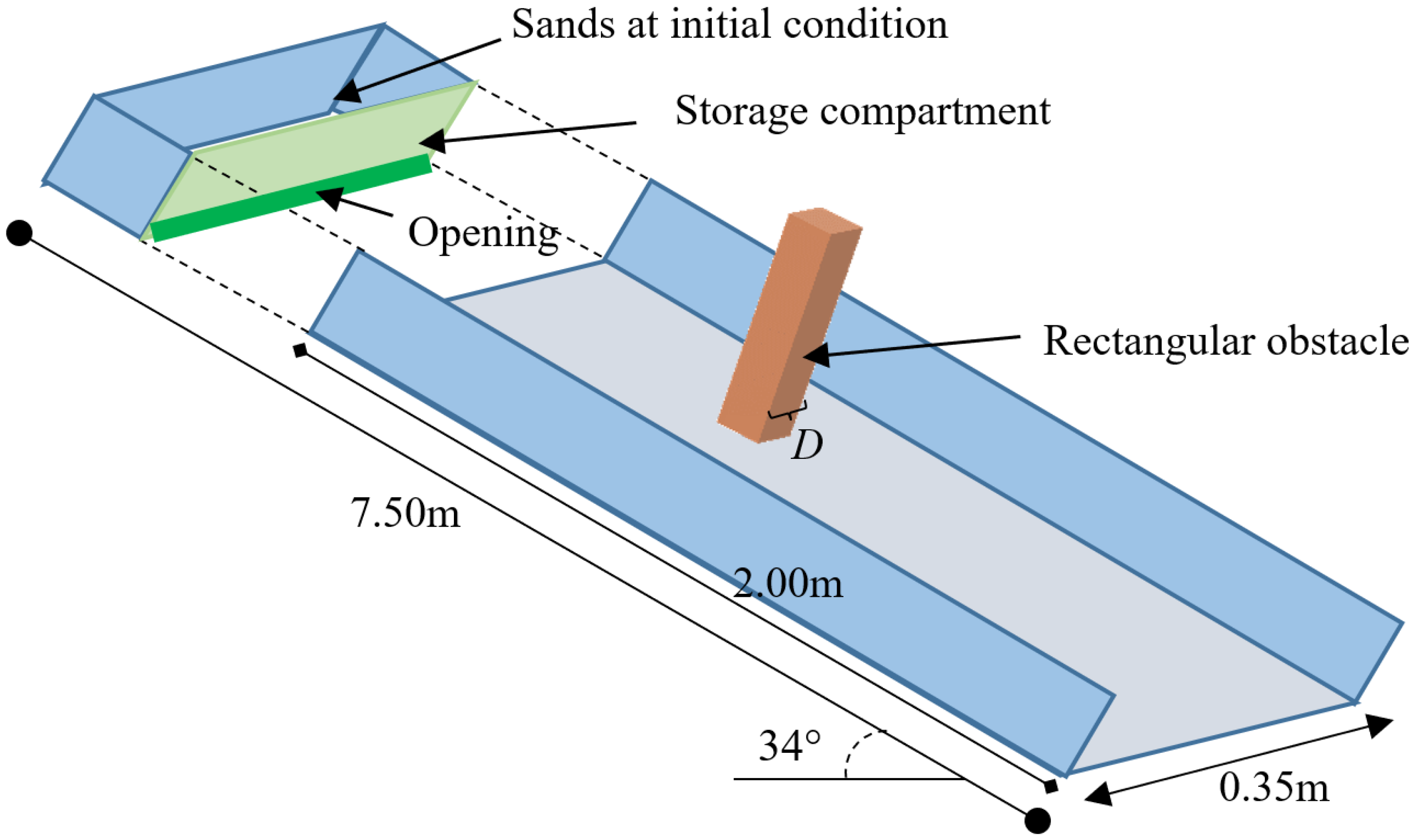
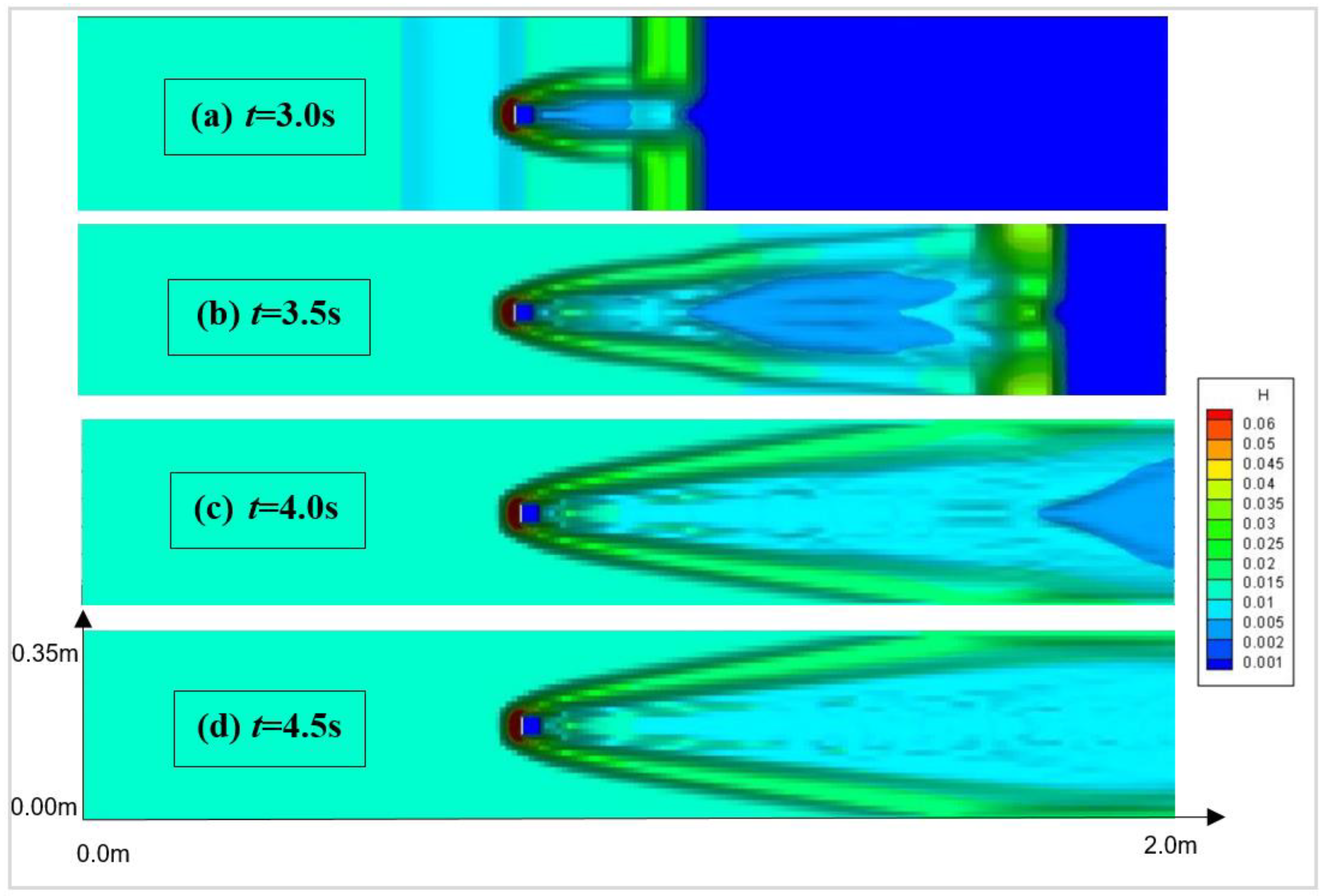
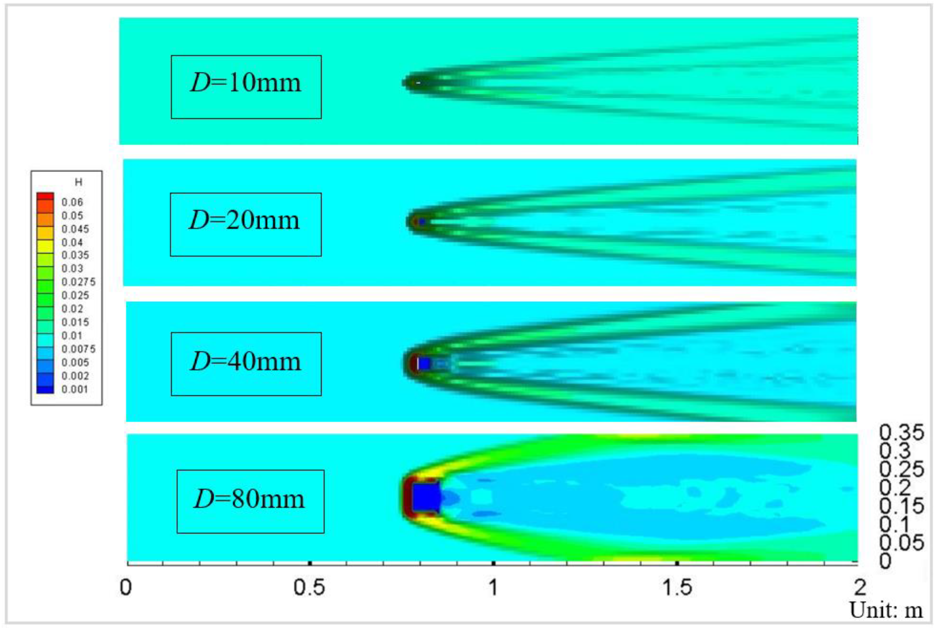
3.1. Granular Flume Flow Strike Mast-Like Obstacle

We simulated the laboratory experiments reported by Hauksson et al. [30], in which grains were initially stored in a compartment and then released within several seconds to simulate a steady granular stream in the chute (Figure 1). The released granular stream would strike rectangular obstacles, which varied in size, i.e., D = 10 mm, 20 mm, 40 mm, and 80 mm, in separate simulations. In the laboratory experiments, the height of the compartment opening was 7 cm, so we fixed the inflow boundary condition as h₀ = 0.07 m in the simulation. Additionally, the natural boundary conditions for the flow velocity were also specified at the inflow and outflow boundaries. The earth pressure coefficients (2b,c) were calculated using the estimated angle of internal friction $\phi$ = 35° and the coefficient of basal friction $\delta$ = 25°, providing the earth pressure coefficient in the x- and y-directions, as follows:

$$K_{x_{act/pas}}=2{\sec }^2\phi \left(1\mp {\left(1-{\cos }^2\phi /{\cos }^2\delta \right)}^{1/2}\right)-1=0.298/5.662,$$

(10a)

$$K_{y_{act/pas}}=\frac{1}{2}\left\{K_x+1\mp {\left[{\left(K_x-1\right)}^2+4{\tan }^2\delta \right]}^{1/2}\right\}=\{\begin{array}{c}0.067\begin{array}{cc}& \end{array}\partial u/\partial x\ge 0,\partial v/\partial y\ge 0\\ \begin{array}{c}\begin{array}{c}1.234\begin{array}{cc}& \end{array}\partial u/\partial x\ge 0,\partial v/\partial y<0\\ 0.954\begin{array}{cc}& \end{array}\partial u/\partial x<0,\partial v/\partial y\ge 0\end{array}\\ 5.708\begin{array}{cc}& \end{array}\partial u/\partial x<0,\partial v/\partial y<0\end{array}\end{array},$$

(10b)

The length of the chute used in the experiment reported by Hauksson et al. [29] was 7.5 m. We cut out a 2 m long section of the chute near where the obstacle was located and developed the configurational evolution of the granular stream striking a square obstacle (D = 40 mm) as viewed from the top (Figure 2). Obvious jumps in the avalanche depth (i.e., shock wave phenomena) upstream from the obstacle at the front of the flow were evident. Downstream of the obstacle, the granular flow parted into two streams, and a “shallow vacuum area” between the two streams behind the obstacle was formed. In Figure 3 (t = 3.5 s) and Figure 4 (t = 4.5 s), the top-view configurations of the fan-shaped stream generated by the granular flow impacting the obstacle highly depend on the width of the obstacle. The simulated opening between the two granular streams grew as the side length of the obstacle increased.

The depth of the granular flow 0.5 m upstream of the obstacle was tracked for t = 10 s from when the flow started, and was compared with the continuous regression curve obtained from the experimental data [30] (Figure 5). The flow depth in the simulation within t = 3 s to 6.5 s was slightly smaller than that in the experiment; however, in general, the simulation results coincided well with the data. The simulated granular flow reached a relatively stable state from t = 4.5 s to 10 s, whereas the depth of the laboratory granular flow stabilized at around 11.5 mm from t = 4 s to 6.5 s, and then declined gradually to 1.8 mm at t = 10 s. The mean square root between the calculated and experimental data was accessed, as shown in Figure 5. The mean square root of the height before t = 6 s was about 1.7991 mm and, during whole process, it was 15.0258 mm. The difference between the simulation and the experiment mainly arose because the experimental granules stocked in the container diminished over time, and the inflow rate in the experiment decreased after t = 6.5 s. In contrast, the inflow rate remained constant in our simulation. We also found that the simulated configurations of the flow remained the same after roughly t = 4.5 s after reaching a “stable state”.

Successive surges (free surface instabilities or rolling waves) have been observed in free surface granular flow on rough inclined planes with glass beads and sands [6,31,32,33] and on smooth inclined planes [34,35]. They correspond to an instability threshold value of roughly 2/3, as defined by the Froude number $Fr=u/\sqrt{gh\cos \theta }$ ($\theta$ the angle of inclination) reported by Forterre [36]. In simulations of avalanche–obstacle interaction with obstacles of different side lengths, we were amazed to find successive waves appearing in the tail of the avalanche between the two streams after t = 5.5 s (Figure 6, area framed by red dashed rectangle). The calculated Froude number at the tail of the flow $Fr\approx 10$ in the simulation was larger than the threshold, which supported the simulation results. Even though (1) and (2) are first-order Saint-Venant-type equations, it was found that second-order effects of successive surges could be reproduced well because of the second-order artificial diffusion term (i.e., total variation diminishing term) added to the simulation.

The computation results of the example in this section indicate that the depth-averaged avalanche dynamics model solved by the TVD-MacCormack scheme captured some basic features of granular flume flow revealed in the laboratory well, such as shock waves and successive surges.

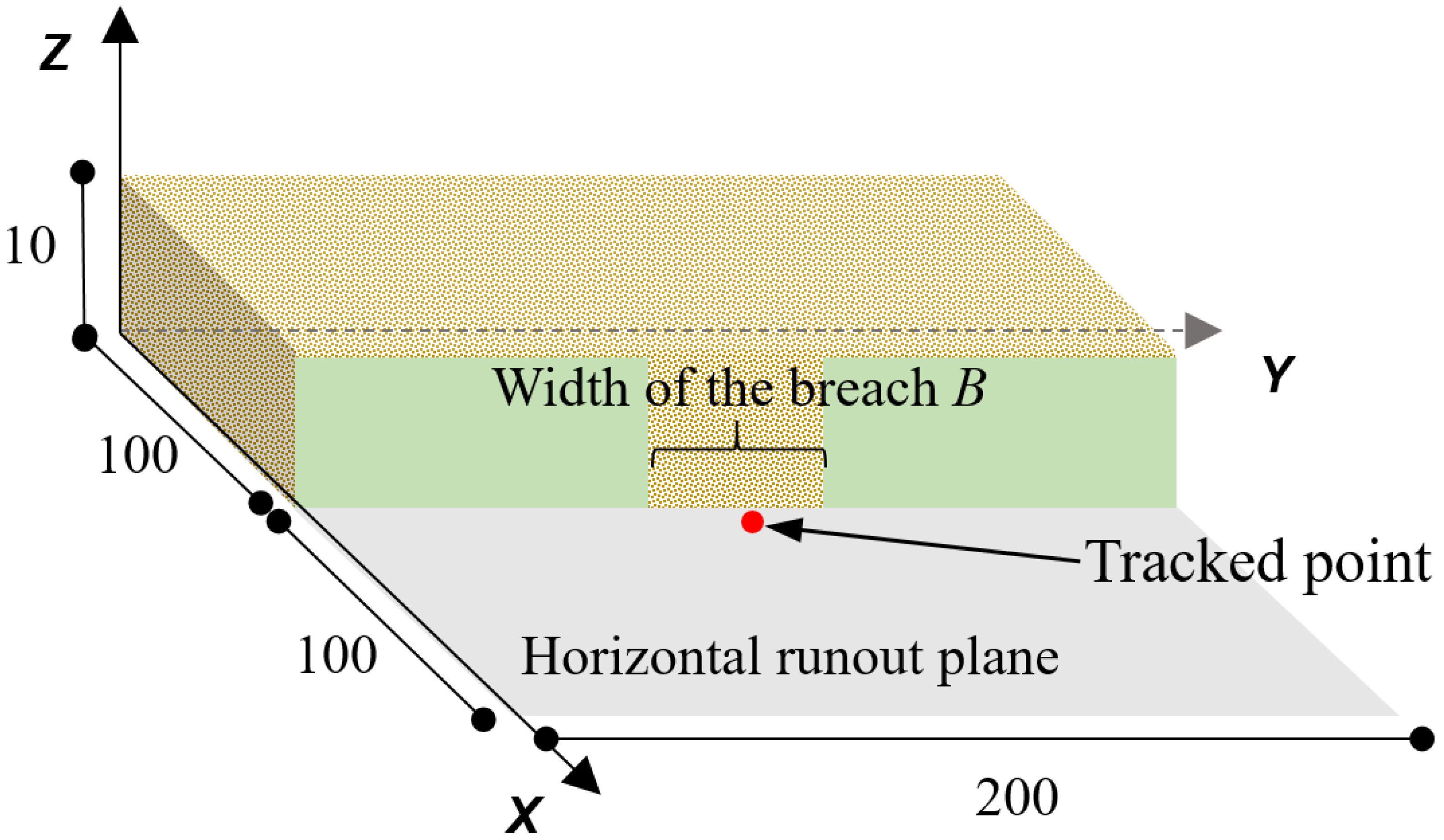
3.2. Granular Dam Break Simulation

Simulations of dam breaking are widely regarded as a benchmark when testing numerical simulation methods [37,38,39]. We simulated a three-dimensional granular version of the dam breaking problem, configured as a box-shaped pile of granular mass initially at rest behind a wall that collapsed with the sudden emergence of a rectangular breach (Figure 7). In the simulation, the calculation domain was 200 m × 200 m and the dimensions of the granular pile were 200 m (width) × 100 m (length) × 10 m (height). We placed the midpoint of the breach at y = 100 m and varied the width of the rectangular breach (B) from 5 m to 10 m, 15 m, 20 m, 35 m, 50 m, and 70 m in separate simulations. The angles of internal friction and coefficient of basal friction were set at $\phi$ = 40° and $\delta$ = 30°, respectively. The earth pressure coefficients were calculated using (10a,b) for the simulations.

The volumetric flow rate per unit width Q (i.e., $\sqrt{{\overline{u}}^2+{\overline{v}}^2}\cdot h\cdot dy$, we used a unit width of dy = 5 m in the simulation), the velocity in the x-direction u, and the granular depth h at x = 105 m and y = 100 m were tracked (Figure 7, red point) during the dam breaking simulations for different breach widths (Figure 8, Figure 9 and Figure 10). From Figure 8 and Figure 9, the flow rate and the velocity in the x-direction with different breach widths all reached large values (Q > 100 m³/s and u > 1.4 m/s) within 3 s, and then decreased rapidly within 10 s. The average values and the fluctuations of the relatively steady flow rate and the velocity after 10 s decreased with the breach width. Figure 10 plots the flow depths at x = 105 m and y = 100 m with time for various breach widths. The depth and its variation decreased with the breach width as well. Larger fluctuations in the flow rate, the velocity, and the depth indicated that the granular mass collapsed more discontinuously with the decrease in breach width. Larger average values for the flow rate and the velocity were likely because more grains flowed over the tracked point, and the duration of dam break process increased with the decrease in breach width.

In the governing equation (i.e., Equations (1) and (2a–e)) used to describe the granular motion, the flow of granules was mainly balanced by the flux vectors and the source terms. Specifically speaking, particles started to move intensively when the depth gradient of the granular flow in the flux vector term exceeded the friction in the source term. The fluctuations in the flow rate, the velocity, and the depth in Figure 8, Figure 9 and Figure 10 indicate that the granular mass collapsed discontinuously. To be specific, the motion of grains remained negligible when the depth gradient of the granular flow was smaller than the friction. As the flow surface gradually grew steeper with the accumulation of grains, an avalanche suddenly occurred when the depth gradient term exceeded the friction term. After the avalanche was terminated, a new balanced state was reached, which is represented by the plateaus in Figure 8, Figure 9 and Figure 10.

According to the results presented in Figure 10, the depth of the mass collapse satisfied a regression model

$$h=h_{\max }\left(1-e^{-t/\tau }\right),$$

(11)

where h_max is a limiting value of the depth and τ is a “relaxation” parameter. We completed a regression analysis based on this dependence, and the fitting parameters of h_max and τ are evaluated and listed in

Table 1. Fitting results of h_max and τ.

Num.	B/m	hmax/m	τ/s
1	5	6.692979	6.90883
2	10	6.135773	6.557069
3	15	9.688248	6.989259
4	20	9.814965	7.037584
5	35	10.08215	6.778386
6	50	11.97468	6.661324
7	70	13.35109	6.441027

.

To check the effect of the boundary condition on the simulation results, we moved the midpoint of the breach to one side, i.e., y = 85 m (B = 70 m), and applied two types of boundary conditions in the simulations: (1) the open boundary (zero-gradient) condition for all four outer boundaries, and (2) the open boundary condition for the boundary adjacent to the dam and the closed boundary for the other three boundaries. The boundary conditions were found to affect the collapse process of the granular pile (Figure 11); the deposit from the opening was mostly grains that were initially adjacent to boundary 1 with the first type of boundary condition, whereas the deposit collapsed evenly for the accumulated grains initially near the opening with the second type of boundary condition.

4. Conclusions and Discussion

The depth-averaged continuum method is an effective approach for solving the avalanche dynamics model. It simplifies all the physical complexity and uncertainty of the motion of a large quantity of grains in a “granular fluid”. Considering the nonlinear properties of the governing equations of the dynamics, developing an accurate and efficient numerical scheme is challenging. We applied the TVD-MacCormack scheme, which was initially used to solve the Saint-Venant equation for shallow water flow. The scheme introduces a TVD term into the MacCormack scheme after the corrector step, enabling second-order spatial and temporal accuracy during the calculation. In addition, the with/without grain algorithm was integrated into the predictor–corrector steps during the computation.

The application of the scheme was checked in two scenarios. The first was a granular flume flow striking square obstacles with varying side lengths splitting into two granular streams. Thus, a fan-shaped configuration formed and the opening between the two granular streams grew with the increasing side length. The simulation results generally agreed well with the laboratory measurements with regard to the granular depth upstream from the obstacle. Using the TVD-MacCormack scheme, we captured shock waves and observed successive waves appearing in the tail of the avalanche between the two streams of flow during the simulations, as observed in previous laboratory research.

In the dam breach simulations, the second scenario, a box-shaped pile of granular mass collapsed following the sudden emergence of a rectangular breach. We changed the width of the breach and tracked the flow rate Q, the velocity u in the x-direction, and the granular depth h during the breaching of the dam. The simulation results indicated that both the flow rate and the velocity in the x-direction reached large values within a short period of time and then decreased rapidly. The average values and the fluctuations of the relatively steady flow rate and the velocity were also found to decrease with the breach width. The results of the granular dam break simulations also revealed that the boundary conditions (open or closed) affected the collapse of the granular pile, i.e., grains evenly breached out under closed boundary conditions, whereas the granules breaching out of the opening were mostly grains adjacent to the boundaries under open boundary conditions.

Although the applied governing equations and the corresponding numerical algorithms have been well developed, the TVD-MacCormack scheme (a second-order spatial and temporal finite-element scheme) was successfully implemented here to solve a two-dimensional dynamics model of a depth-averaged avalanche with high accuracy. In addition, the simulation of a granular flume flow–obstacle interaction scenario and a granular dam breaking scenario captured some valuable features in these two scenarios, i.e., shock waves with a fan-shaped configuration and successive waves in the tail of the avalanche between the two streams in the first scenario, as well as discontinuous granular collapses in the second scenario. Capturing these two complex and typical granular-flow phenomena indicates the applicability and effectiveness of combining the TVD-MacCormack scheme and S-H model to simulate dam breaking and inclined flow–obstacle interaction cases.

This paper investigates what happens when a dense granular flow strikes on a rigid obstacle, described by a wall boundary, rather than a topographic feature with a finite slope. It is shown that the numerical method of the TVD-MacCormack scheme has a shock-capturing ability and can be used to solve for the motion of granular dam breaking. The granular flow–obstacle interaction case uses a rectangular cylinder as an obstacle, which is not the classical circular shape. This is of practical interest for the design of defending structures that can withstand such avalanches. In addition, it can represent natural obstacles such as trees. The dam breaking scenario may provide basic physical insight into the problem in which a vertical retaining wall breaks, and thus the granular cliff collapses gradually. Simulated discontinuous granular mass collapses are consistent with the observation on the failure process of a natural slope.

The absence of an obstacle generates adjacent shock waves, at which point there are rapid changes in the granular flow thickness and flow velocity. Shock waves arise naturally from the hyperbolic structure of the Saint-Venant equations. In diluted granular flows, shock waves high in density develop and the diluted flow can be seen as compressible flow. This paper investigates dense granular flow with a low solid volume fraction that travels past obstacles, and the flow is modelled as an incompressible flow.

References

1. Maccormack, R.W. An efficient explicit–implicit–characteristic method for solving the compressible Navier–Stokes equations. SIAM–AMS Proc. 1978, 11, 130–155. [Google Scholar]
2. Savage, S.B.; Hutter, K. The motion of a finite mass of granular material down a rough incline. J. Fluid Mech. 1989, 199, 177–215. [Google Scholar] [CrossRef]
3. Anderson, D.A.; Tannehill, J.C.; Pletcher, R.H. Computational Fluid Mechanics and Heat Transfer; McGraw-Hill Book Company: New York, NY, USA, 1984. [Google Scholar]
4. Ferrand, M.; Harris, J.C. Finite volume arbitrary Lagrangian-Eulerian schemes using dual meshes for ocean wave applications. Comput. Fluids 2021, 219, 104860. [Google Scholar] [CrossRef]
5. Huang, C.S.; Arbogast, T.; Hung, C.H. A semi-Lagrangian finite difference WENO scheme for scalar nonlinear conservation laws. J. Comput. Phys. 2016, 322, 559–585. [Google Scholar] [CrossRef] [Green Version]
6. Forterre, Y.; Pouliquen, O. Long–surface–wave instability in dense granular flows. J. Fluid Mech. 2003, 486, 21–50. [Google Scholar] [CrossRef] [Green Version]
7. Tai, Y.C.; Gray, J.M.N.T.; Hutter, K.; Noelle, S. Flow of dense avalanches past obstructions. Ann. Glaciol. 2001, 32, 281–284. [Google Scholar] [CrossRef] [Green Version]
8. Cui, X. Computational and experimental studies of rapid free–surface granular flows around obstacles. Comput. Fluids 2014, 89, 179–190. [Google Scholar] [CrossRef]
9. Abdelrazek, A.M.; Kimura, I.; Shimizu, Y. Numerical simulation of granular flow past simple obstacles using the SPH method. J. Jpn. Soc. Civ. Eng. Ser. B1 2015, 71, 199–204. [Google Scholar] [CrossRef] [Green Version]
10. Saghi, H.; Lakzian, E. Effects of using obstacles on the dam-break flow based on entropy generation analysis. Eur. Phys. J. Plus 2019, 134, 237. [Google Scholar] [CrossRef]
11. Nessyahu, H.; Tadmor, E. Non–oscillatory central differencing for hyperbolic conservation laws. J. Comput. Phys. 1990, 87, 408–463. [Google Scholar] [CrossRef] [Green Version]
12. Balbás, J.; Tadmor, E.; Wu, C.C. Non–oscillatory central schemes for one–and two–dimensional MHD equations. J. Comput. Phys. 2004, 201, 261–285. [Google Scholar] [CrossRef]
13. Kurganov, A.; Tadmor, E. New high–resolution semi–discrete central schemes for Hamilton–Jacobi equations. J. Comput. Phys. 2000, 160, 720–742. [Google Scholar] [CrossRef] [Green Version]
14. Liu, Y. Central schemes on overlapping cells. J. Comput. Phys. 2005, 209, 82–104. [Google Scholar] [CrossRef]
15. Gray, J.M.N.T.; Tai, Y.C.; Noelle, S. Shock waves, dead zones and particle–free regions in rapid granular free–surface flows. J. Fluid Mech. 2003, 491, 161–181. [Google Scholar] [CrossRef] [Green Version]
16. Tai, Y.C.; Noelle, S.; Gray, J.M.N.T.; Hutter, K. Shock–capturing and front–tracking methods for granular avalanches. J. Comput. Phys. 2002, 175, 269–301. [Google Scholar] [CrossRef] [Green Version]
17. Pitman, E.B.; Nichita, C.C.; Patra, A.; Bauer, A.; Sheridan, M.; Bursik, M. Computing granular avalanches and landslides. Phys. Fluids 2003, 15, 3638–3646. [Google Scholar] [CrossRef] [Green Version]
18. Denlinger, R.P.; Iverson, R.M. Flow of variably fluidized granular masses across three-dimensional terrain: 2. Numerical predictions and experimental tests. J. Geophys. Res.-Solid Earth 2001, 106, 553–566. [Google Scholar] [CrossRef]
19. Jeong, K.L.; Lee, Y.G. A numerical simulation method for the flow around floating bodies in regular waves using a three-dimensional rectilinear grid system. Int. J. Nav. Archit. Ocean. Eng. 2016, 8, 277–300. [Google Scholar] [CrossRef] [Green Version]
20. Ferreira, D.M.; Fernandes, C.V.S.; Kaviski, E.; Bleninger, T. Calibration of river hydrodynamic models: Analysis from the dynamic component in roughness coefficients. J. Hydrol. 2021, 598, 126136. [Google Scholar] [CrossRef]
21. Heer, T.; Wells, M.G.; Mandrak, N.E. Asian carp spawning success: Predictions from a 3-D hydrodynamic model for a Laurentian Great Lake tributary. J. Great Lakes Res. 2021, 47, 37–47. [Google Scholar] [CrossRef]
22. Zhang, X.X.; Li, D.; Wang, X.; Li, X.; Cheng, J.Y.; Zheng, B.Z. Exploration of polycyclic aromatic hydrocarbon distribution in the sediments of marine environment by hydrodynamic simulation model. Mar. Pollut. Bull. 2021, 171, 112697. [Google Scholar] [CrossRef]
23. Tai, Y.C.; Kuo, C.Y.; Hui, W.H. An alternative depth–integrated formulation for granular avalanches over temporally varying topography with small curvature. Geophys. Astrophys. Fluid Dyn. 2012, 106, 596–629. [Google Scholar] [CrossRef]
24. Murillo, C.J.J.; García-Navarro, P. 2D simulation of granular flow over irregular steep slopes using global and local coordinates. J. Comput. Phys. 2013, 255, 166–204. [Google Scholar]
25. Mingham, C.G.; Causon, D.M.; Ingram, D.M. A TVD MacCormack scheme for transcritical flow. ICE Proc. Water Marit. Eng. 2001, 148, 167–175. [Google Scholar] [CrossRef]
26. Liang, D.; Falconer, R.A.; Lin, B. Comparison between TVD-MacCormack and ADI-type solvers of the shallow water equations. Adv. Water Resour. 2006, 29, 1833–1845. [Google Scholar] [CrossRef]
27. Liang, D.; Lin, B.; Falconer, R.A. Simulation of rapidly varying flow using an efficient TVD–MacCormack scheme. Int. J. Numer. Methods Fluids 2007, 53, 811–826. [Google Scholar] [CrossRef]
28. Khodadosti, F.; Khalsaraei, M.M. A new total variation diminishing implicit nonstandard finite difference scheme for conservation laws. Comput. Methods Differ. Equ. 2014, 2, 91–98. [Google Scholar]
29. Zendrato, N.L.H.; Chrysanti, A.; Yakti, B.P.; Adityawan, M.B.; Suryadi, Y. Application of finite difference schemes to 1D St. venant for simulating weir overflow. MATEC Web Conf. 2018, 147, 03011. [Google Scholar] [CrossRef] [Green Version]
30. Hauksson, S.; Pagliardi, M.; Barbolini, M.; Johannesson, T. Laboratory measurements of impact forces of supercritical granular flow against mast–like obstacles. Cold Reg. Sci. Technol. 2007, 49, 54–63. [Google Scholar] [CrossRef]
31. Shirsath, S.S.; Padding, J.T.; Deen, N.G.; Clercx, H.J.H.; Kuipers, J.A.M. Experimental study of monodisperse granular flow through an inclined rotating chute. Powder Technol. 2013, 246, 235–246. [Google Scholar] [CrossRef]
32. Ionescu, I.R.; Mangeney, A.; Bouchut, F.; Roche, O. Viscoplastic modeling of granular column collapse with pressure-dependent rheology. J. Non-Newton. Fluid Mech. 2015, 219, 1–18. [Google Scholar] [CrossRef]
33. Daerr, A. Dynamical equilibrium of avalanches on a rough plane. Phys. Fluid 2001, 13, 2115–2124. [Google Scholar] [CrossRef] [Green Version]
34. Prasad, S.N.; Pal, D.; Romkens, M.J.M. Wave formation on a shallow layer of flowing grains. J. Fluid Mech. 2000, 413, 89–110. [Google Scholar] [CrossRef]
35. Louge, M.Y.; Keast, S.C. On dense granular flows down flat frictional inclines. Phys. Fluids 2001, 13, 1213–1233. [Google Scholar] [CrossRef]
36. Forterre, Y. Kapiza waves as a test for three–dimensional granular flow rheology. J. Fluid Mech. 2006, 563, 123. [Google Scholar] [CrossRef] [Green Version]
37. Johannesson, T.; Gauer, P.; Issler, D.; Lied, K.; Faug, T.; Naaim, M. The Design of Avalanche Protection Dams. Recent Practical and Theoretical Developments; European Commission, Directorate General for Research: Bruxelles, Belgium, 2009. [Google Scholar]
38. Saghi, H.; Ketabdari, M.J.; Zamirian, M. A novel algorithm based on parameterization method for calculation of curvature of the free surface flows. Modelling 2013, 37, 570–585. [Google Scholar] [CrossRef] [Green Version]
39. Saghi, H.; Hashemian, A. Multi-dimensional NURBS model for predicting maximum free surface oscillation in swaying rectangular storage tanks. Comput. Math. Appl. 2018, 76, 2496–2513. [Google Scholar] [CrossRef]
Figure 1. Schematic of the laboratory installation; grains initially stored in a compartment were released from a 70 mm high opening to simulate a granular stream striking a rectangular obstacle during the flow process.
Applsci 12 05066 g001
Figure 2. Simulated flow process of a uniform granular stream hitting a square obstacle with a side length of 0.04 m: (a) t = 3.0 s, (b) t = 3.5 s, (c) t = 4.0 s, and (d) t = 4.5 s (unit: m).
Applsci 12 05066 g002
Figure 3. Configurational comparison of an avalanche hitting a square obstacle with different side lengths at time t = 3.5 s.
Applsci 12 05066 g003
Figure 4. Configurations of an avalanche hitting an obstacle with different side lengths at time t = 4.5 s.
Applsci 12 05066 g004
Figure 5. Comparison of laboratory data and simulation results (the continuous regression curve is obtained from experimental data in Hauksson et al. (2007), and the orange square dots are the simulation data).
Applsci 12 05066 g005
Figure 6. Successive surges in the tail of the fan captured during simulations obtained using the proposed numerical scheme.
Applsci 12 05066 g006
Figure 7. Schematic of the box-shaped pile of granular mass before collapse through a rectangular breach into a horizontal runout plane (unit: m).
Applsci 12 05066 g007
Figure 8. Changes in volumetric flow rate per unit width at the track point marked in Figure 7 over time for different breach widths.
Applsci 12 05066 g008
Figure 9. Plots of tracked velocity in the x-direction with different breach widths during dam breaking.
Applsci 12 05066 g009
Figure 10. Tracked depth of the mass collapse from a breach of different widths during the dam breaking process.
Applsci 12 05066 g010
Figure 11. Comparison of the computational dam break configuration at times t = 40 s (upper) and t = 80 s (lower) with open (left) and closed (right) boundary conditions (unit: m).
Applsci 12 05066 g011