
Prediction of Soil Shear Strength Parameters Using Combined Data and Different Machine Learning Models

 ,
,
Abstract
:1. Introduction
2. Materials and Methods
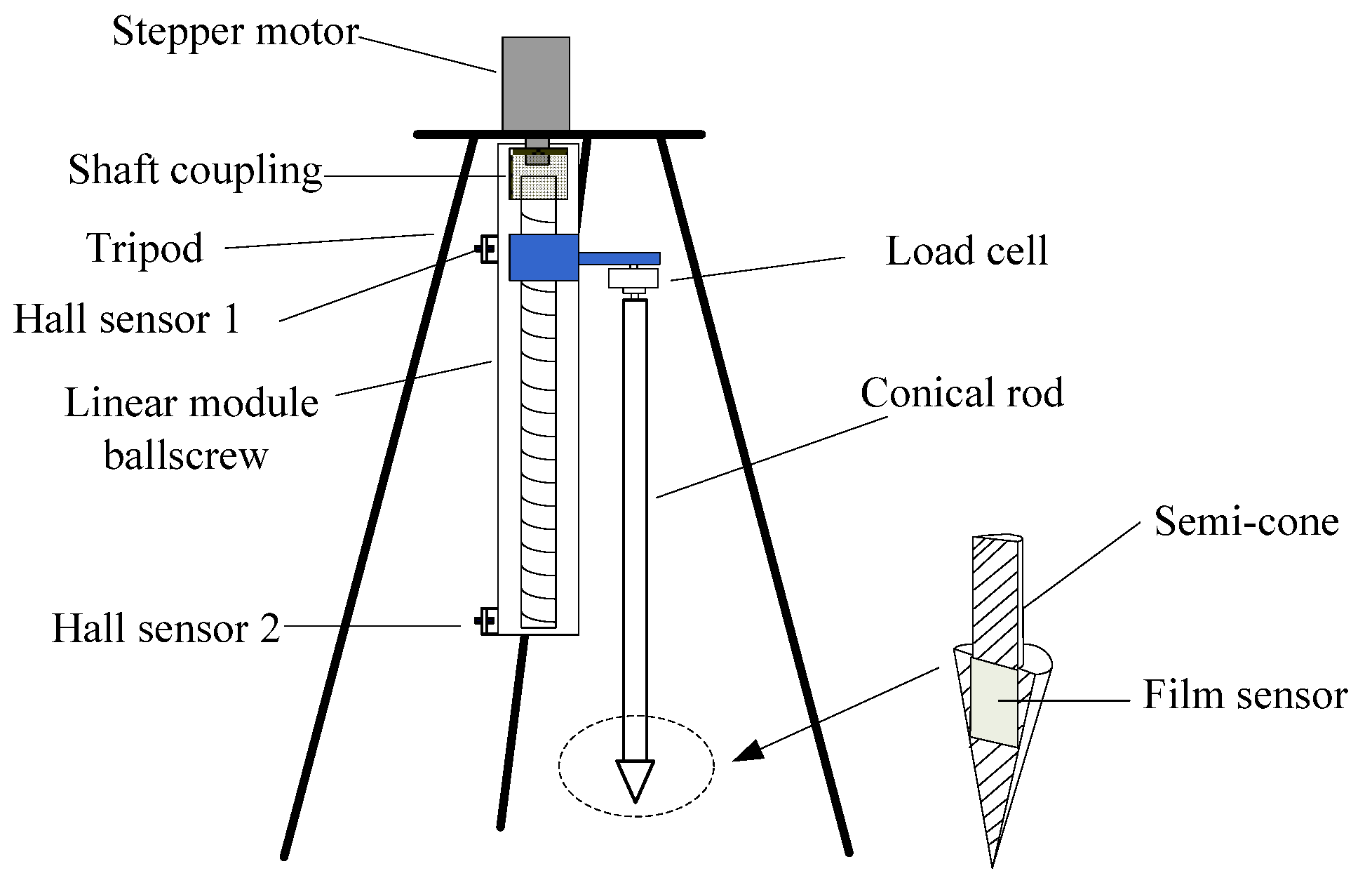
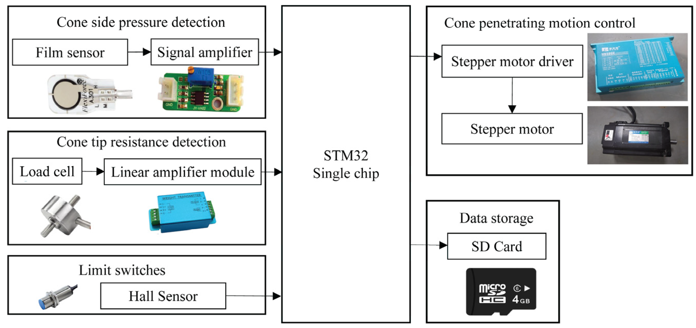
2.1. Instruments
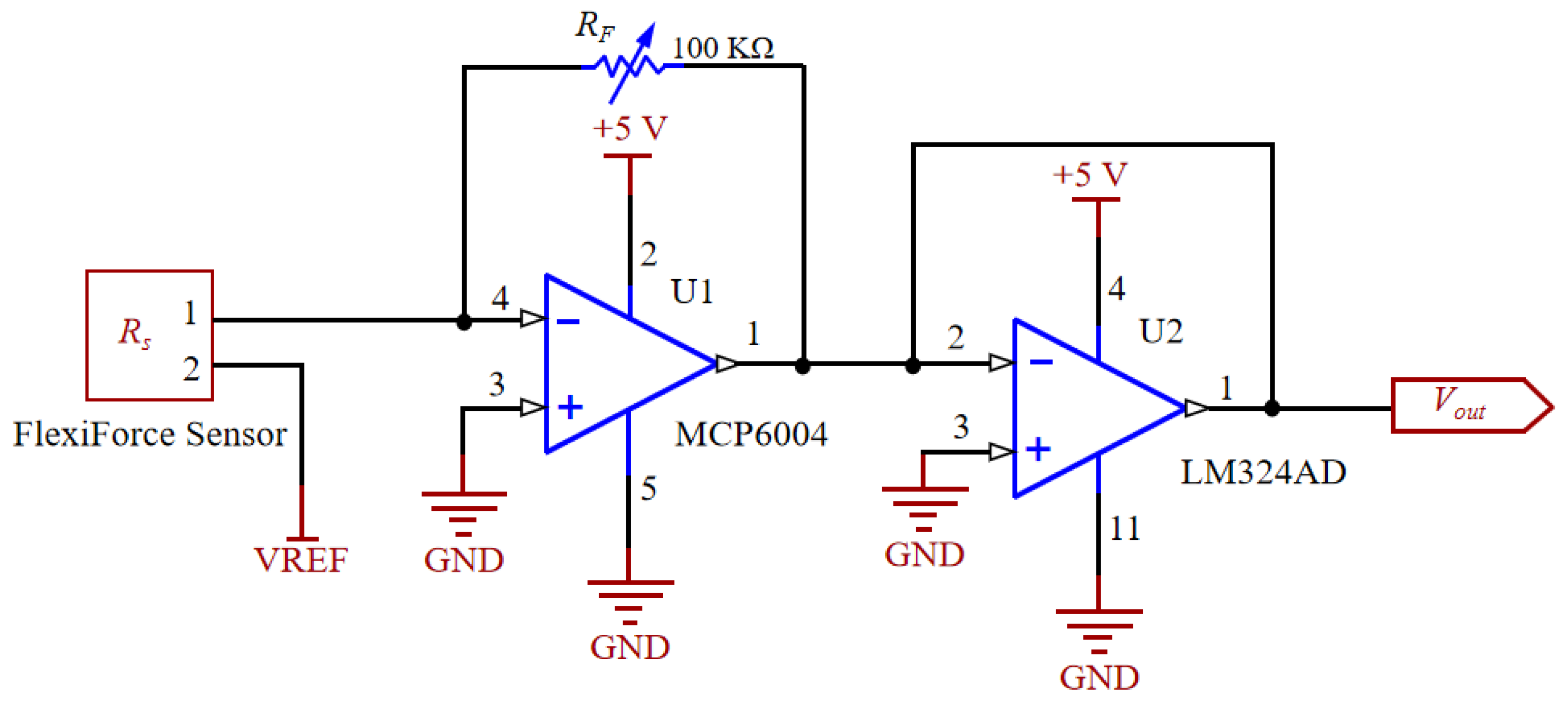
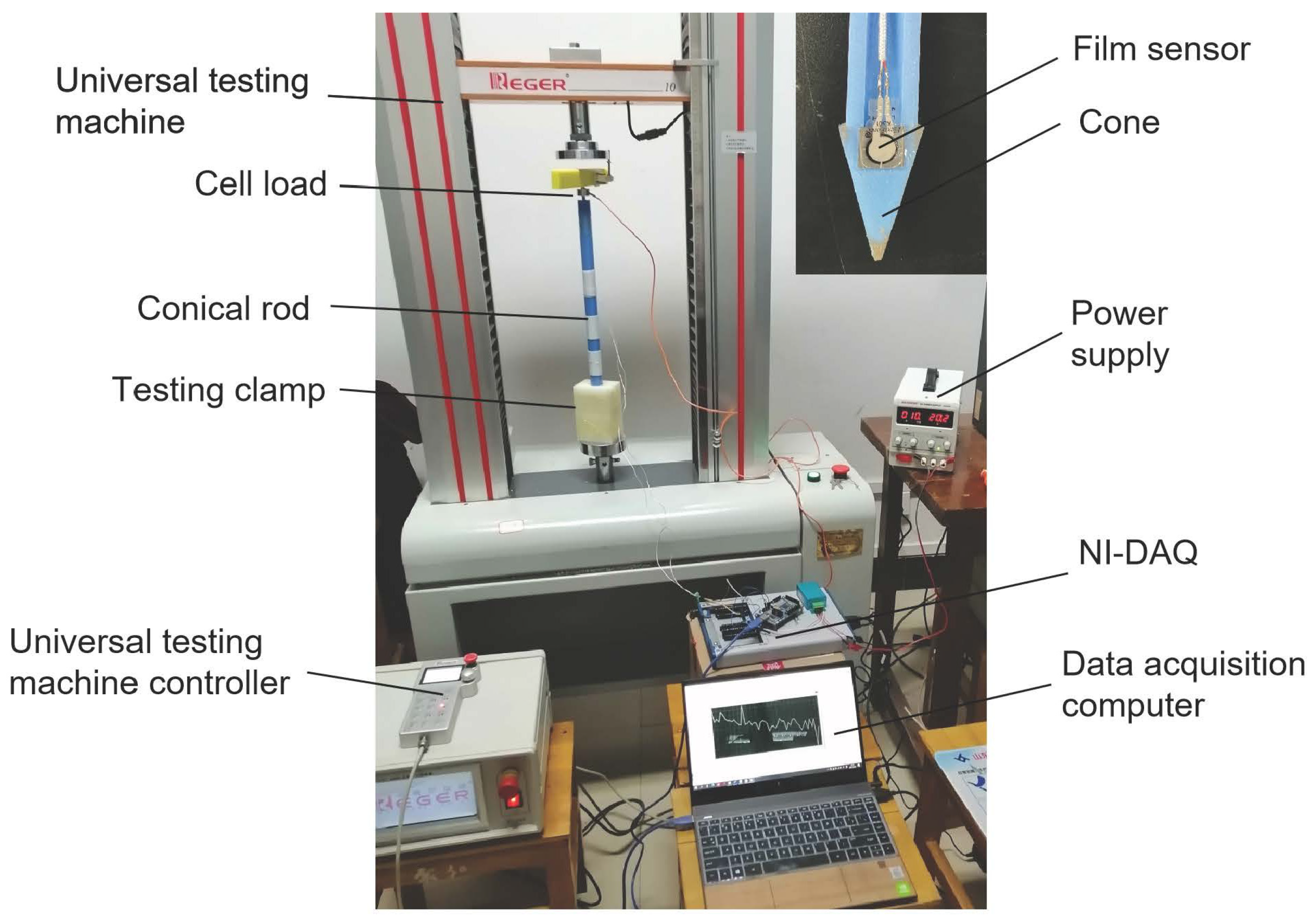
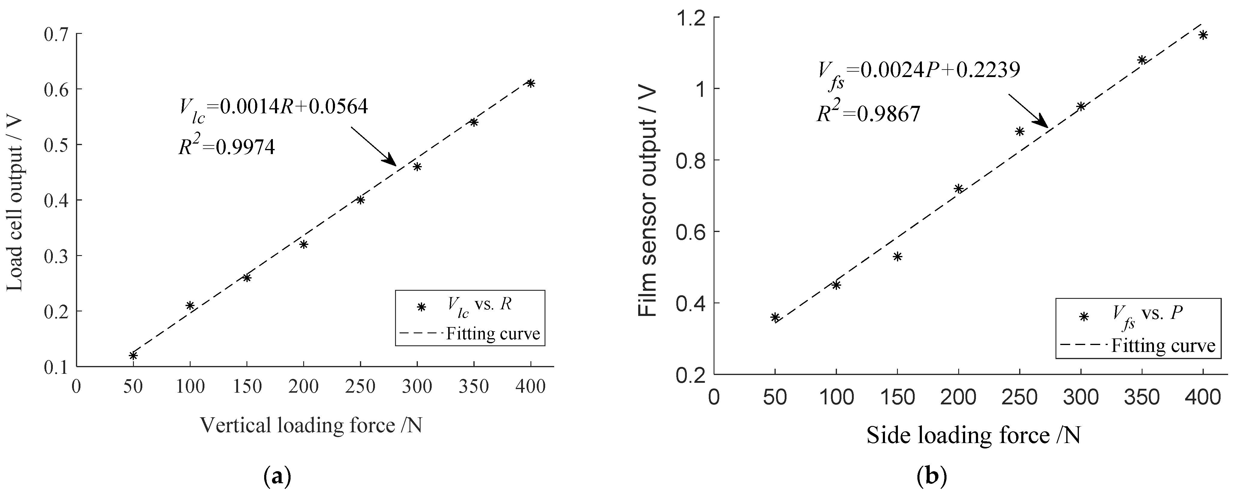
2.2. Sensors Calibration
2.3. Data Collection and Data Set Construction
2.3.1. Soil Sampling and Data Measurement
2.3.2. Dataset Construction
2.4. Proposed Machine Learning Models
- (1)
- The constructed dataset is divided into a calibration set and a validation set.
- (2)
- The key parameters of the ML models are determined using optimization methods.
- (3)
- Using the calibration set and determined modeling parameters, a prediction model is built by applying ML algorithms.
- (4)
- The trained ML models are used to predict the validation set.
- (5)
- The performance of each constructed model is evaluated based on the calculation of the predicted and the true value.
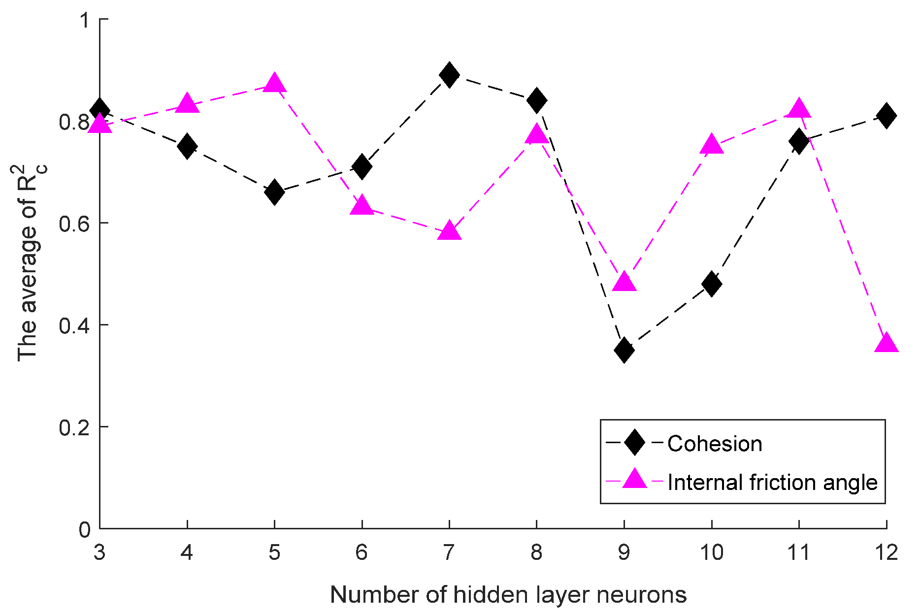
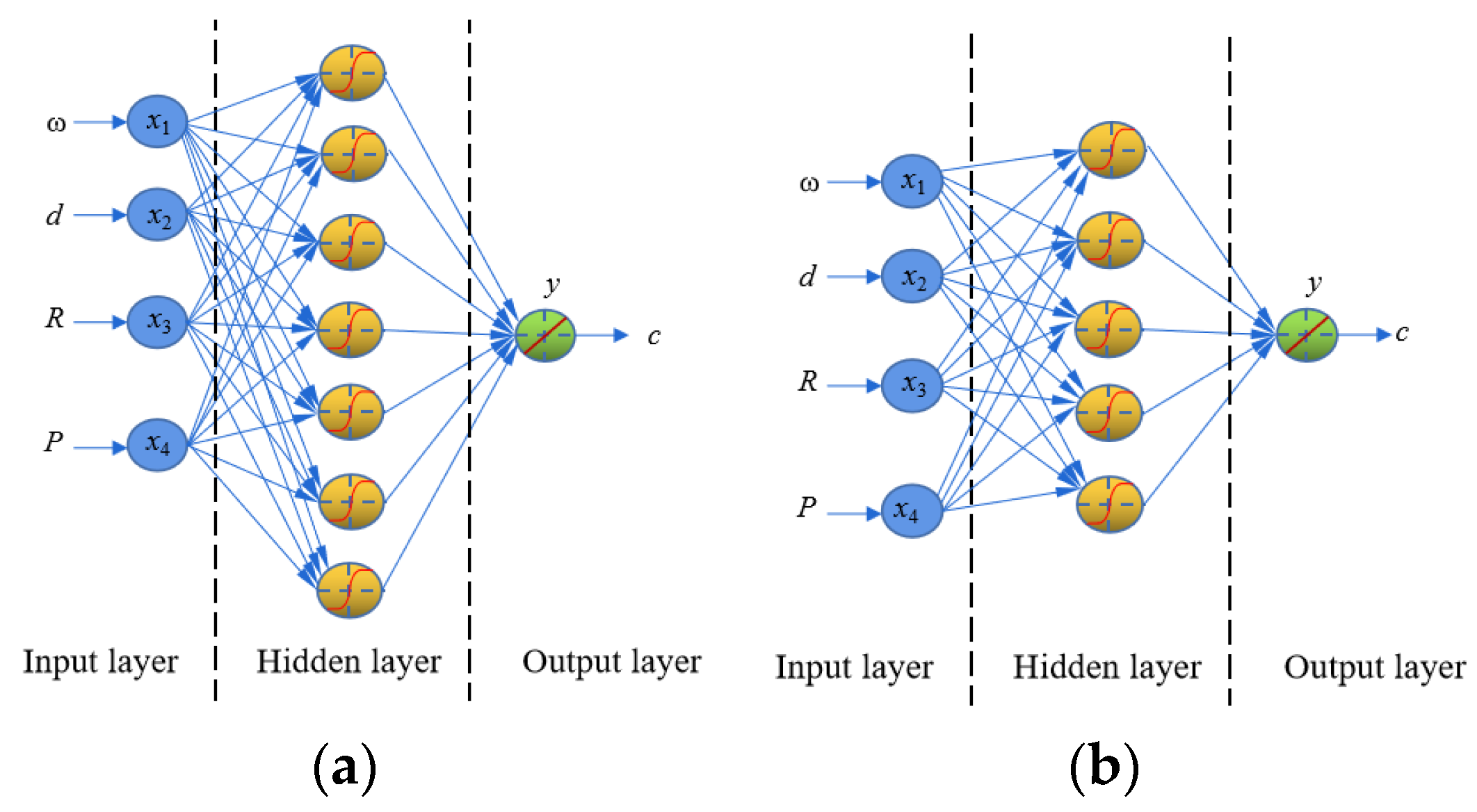
2.4.1. BPNN Model
- (1)
- For each h value within the range, a BPNN model is built, and the calibration set is tested 10 times by the BPNN.
- (2)
- The Rc2 corresponding to each test is calculated, and the average value of Rc2 corresponding to each h value is counted.
- (3)
- The optimal h value of modeling is determined according to the average value of Rc2. The larger the Rc2, the better the model.
2.4.2. PLSR Model
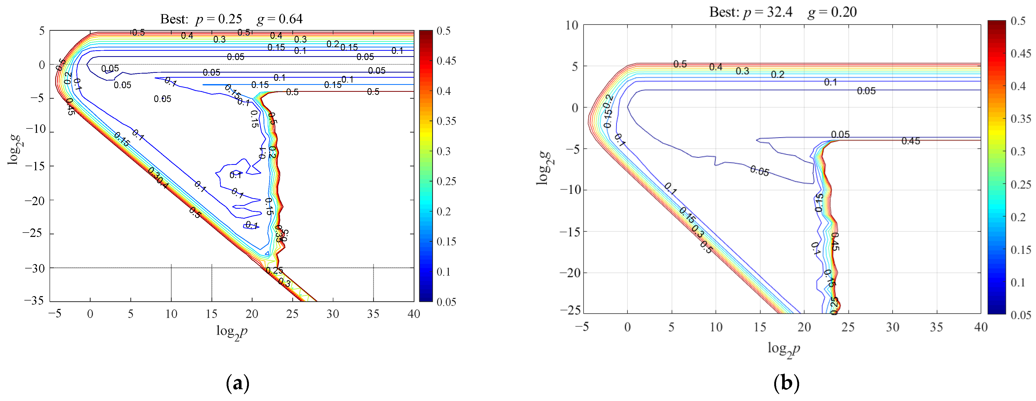
2.4.3. SVR Model
- (1)
- Give wide initial ranges so that p and g are both within 2−40 and 240.
- (2)
- Create grids with small step-by-step values based on the initial ranges.
- (3)
- Using the five-fold cross-validation, select the optimal values of p and g through the mean square error of cross-validation (MSECV). A smaller MSECV means a better combination of p and g.
2.5. Datasets Division
2.6. Performance Evaluation
3. Results
3.1. Results of Measurements and Correlation Analysis
3.2. Results of Model Prediction
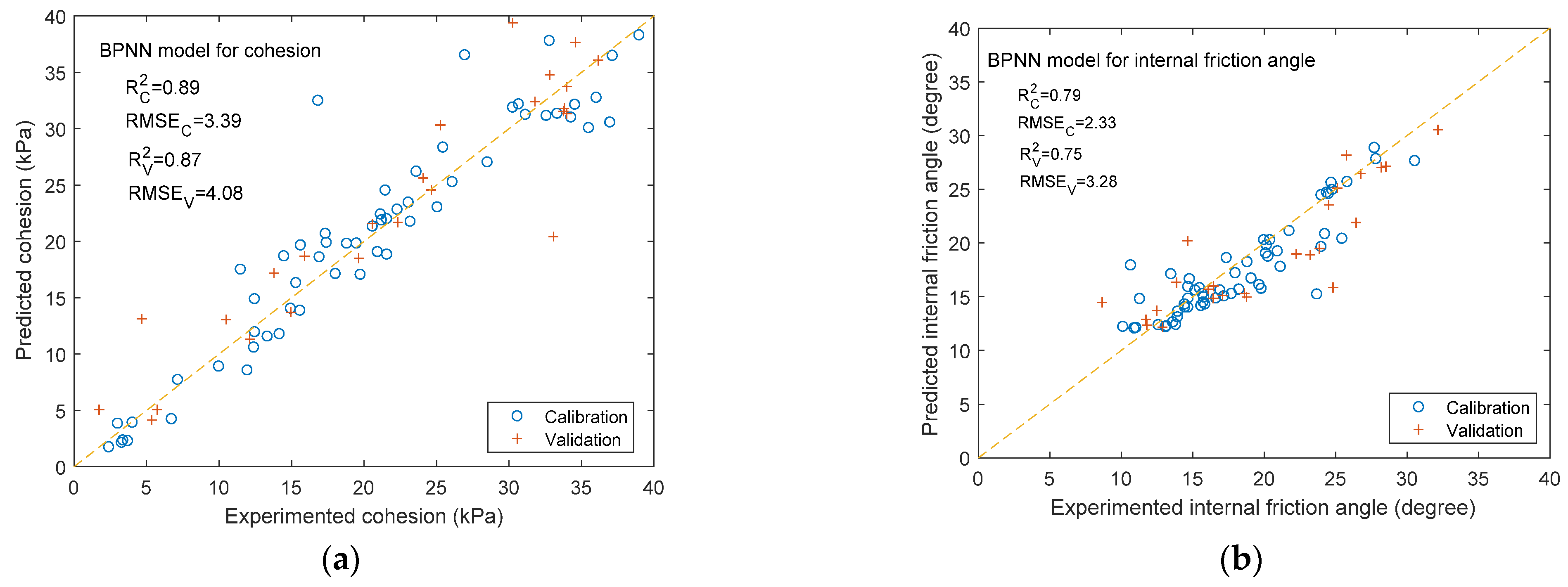
3.2.1. Results of BPNN Model Prediction
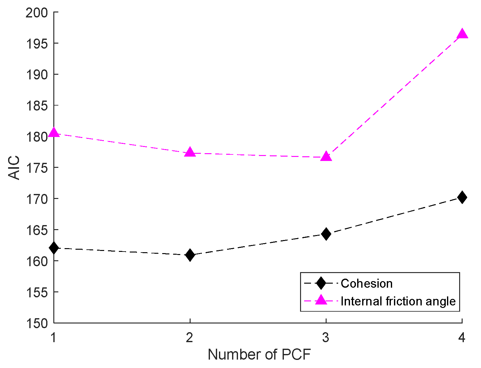
3.2.2. Results of PLSR Model Prediction
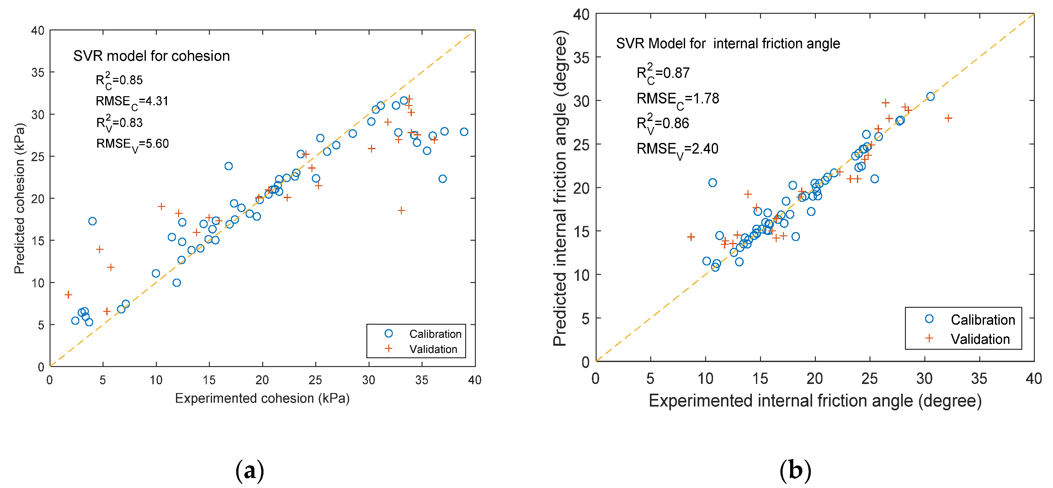
3.2.3. Results of SVR Model Prediction
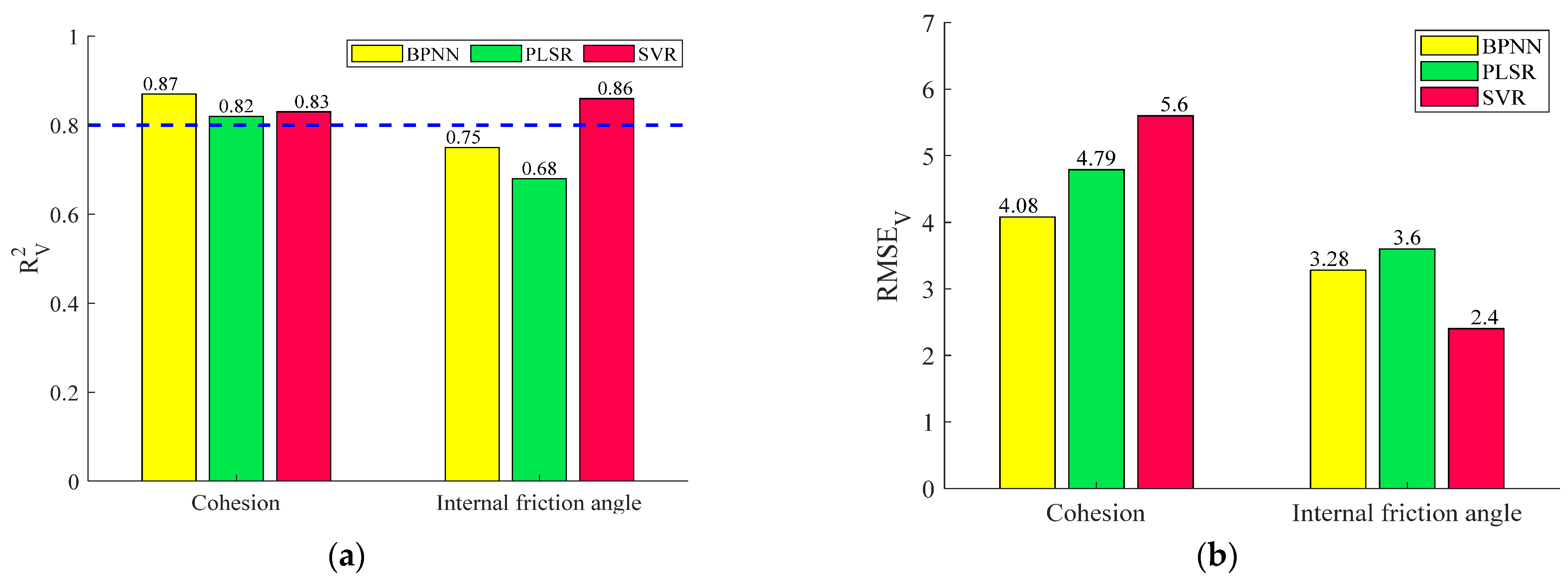
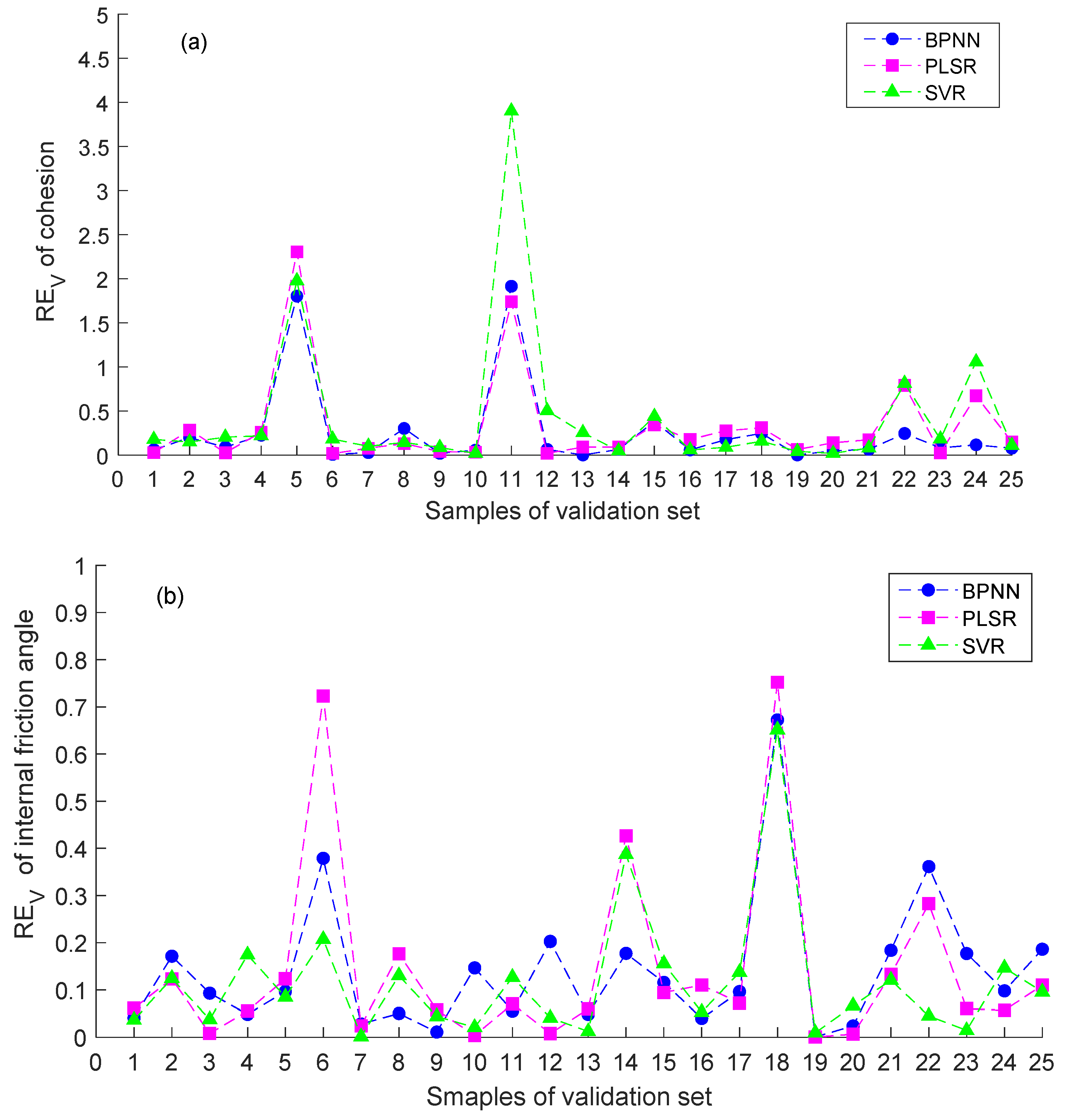
3.3. Comparative Analysis of the Forecasting Performances of the Different Models
4. Conclusions
Author Contributions
Funding
Institutional Review Board Statement
Informed Consent Statement
Data Availability Statement
Conflicts of Interest
References
- Moayedi, H.; Bui, D.T.; Dounis, A. Novel Nature-Inspired Hybrids of Neural Computing for Estimating Soil Shear Strength. Appl. Sci. 2019, 9, 4643. [Google Scholar] [CrossRef] [Green Version]
- Khaboushan, E.A.; Emami, H.; Mosaddeghi, M.R. Estimation of unsaturated shear strength parameters using easily-available soil properties. Soil Tillage Res. 2018, 184, 118–127. [Google Scholar] [CrossRef]
- Barbhuiya, G.H.; Hasan, S.D. Effect of nano-silica on physio-mechanical properties and microstructure of soil: A comprehensive review. Mater. Today Proc. 2021, 44, 217–221. [Google Scholar] [CrossRef]
- Imhoff, S.; Da Silva, A.P.; Fallow, D. Susceptibility to compaction, load support capacity, and soil compressibility of Hapludox. Soil Sci. Soc. 2004, 68, 17–24. [Google Scholar] [CrossRef]
- Schjønning, P.; Lamandé, M.; Keller, T. Subsoil shear strength—Measurements and prediction models based on readily available soil properties. Soil Till. Res. 2020, 200, 104638. [Google Scholar] [CrossRef]
- Blanco-Canqui, H.; Lal, R.; Owen, L.B.; Post, W.M.; Izaurralde, R.C. Strength properties and organic carbon of soils in the north appalachian region. Soil Sci. Soc. Am. J. 2005, 69, 663–673. [Google Scholar] [CrossRef]
- Stafford, J.V.; Tanner, D.W. Effect of rate on soil shear strength and soil-metal friction I. Shear strength. Soil Tillage Res. 1983, 3, 245–260. [Google Scholar] [CrossRef]
- Eudoxie, G.D.; Phillips, D.; Springer, R. Surface hardness as an indicator of soil strength of agricultural soils. Open J. Soil Sci. 2012, 2, 341–346. [Google Scholar] [CrossRef] [Green Version]
- Bradford, J.M.; Grossman, R.B. In-situ measurement of near-surface soil strength by the fall-cone device. Soil Sci. Soc. Am. J. 1982, 46, 685–688. [Google Scholar] [CrossRef]
- Wuddivira, M.N.; Stone, R.J.; Ekwue, E.I. Influence of cohesive and disruptive forces on strength and erodibility of tropical soils. Soil Tillage Res. 2013, 133, 40–48. [Google Scholar] [CrossRef]
- Khalili, N.; Geiser, F.; Blight, G.E. Effective stress in unsaturated soils: Review with new evidence. Int. J. Geomech. 2004, 4, 115–126. [Google Scholar] [CrossRef]
- Brzezinski, K.; Jozefiak, K.; Zbiciak, A. On the interpretation of shear parameters uncertainty with a linear regression approach. Measurement 2021, 174, 108949. [Google Scholar] [CrossRef]
- Bol, E.; Onalp, A.; Ozocak, A.; Sert, S. Estimation of the undrained shear strength of Adapazari fine grained soils by cone penetration test. Eng. Geol. 2019, 261, 105277. [Google Scholar] [CrossRef]
- Begemann, H.K. The friction jacket cone as an aide in determining the soil profile. In Proceedings of the 6th International Conference on Soil Mechanics and Foundation Engineering, Montreal, QC, Canada, 8–15 September 1965; Volume 1, pp. 17–20. [Google Scholar]
- Salari, P.; Lashkaripour, G.; Ghafoori, M. Presentation of empirical equations for estimating internal friction angle of SP and SC soils in Mashhad, Iran using standard penetration and direct shear tests and comparison with previous equations. Int. J. Geogr. Geol. 2015, 4, 89–95. [Google Scholar] [CrossRef] [Green Version]
- Motaghedi, H.; Armaghani, D.J. New method for estimation of soil shear strength parameters using results of piezocone. Measurement 2016, 77, 132–142. [Google Scholar] [CrossRef]
- Satyanaga, A.; Bairakhmetov, N.; Kim, J.R.; Moon, S.W. Role of bimodal water retention curve on the unsaturated shear strength. Appl. Sci. 2022, 12, 1266. [Google Scholar] [CrossRef]
- García, A.J.H.; Jaime, Y.N.M. Savanna soil water content effect on its shear strength-compaction relationship. Rev. Cient. Agric. 2013, 12, 324–337. [Google Scholar]
- Zheng, Z.; Zhang, X.; Li, T.; Jin, W.; Lin, C. Change characteristics and influencing factors of soil shear strength during maize growing period. Trans. Chin. Soc. Agric. Mach. 2014, 45, 125–130. [Google Scholar] [CrossRef]
- Zhang, B.; Zhao, Q.G.; Horn, R.; Baumgartl, T. Shear strength of surface soil as affected by soil bulk density and soil water content. J. Soil Tillage Res. 2001, 34, 162–174. [Google Scholar] [CrossRef]
- Stefanow, D.; Dudziński, P.A. Soil shear strength determination methods–State of the art. Soil Till. Res. 2021, 208, 104881. [Google Scholar] [CrossRef]
- Baldi, P.; Brunak, S. Bioinformatics: The machine learning approach. Phys. Today 2002, 55, 57–58. [Google Scholar] [CrossRef]
- Li, G.; Li, Y.; Chen, H.; Deng, W. Fractional-order controller for course-keeping of underactuated surface vessels based on frequency domain specification and improved particle swarm optimization algorithm. Appl. Sci. 2022, 12, 3139. [Google Scholar] [CrossRef]
- Lee, M.; Jeon, I.; Jun, C. A deterministic methodology using smart card data for prediction of ridership on public transport. Appl. Sci. 2022, 12, 3867. [Google Scholar] [CrossRef]
- Cui, H.; Guan, Y.; Chen, H. Rolling element fault diagnosis based on VMD and sensitivity MCKD. IEEE Access 2021, 9, 120297–120308. [Google Scholar] [CrossRef]
- Özçoban, M.Ş.; Isenkul, M.E.; Sevgen, S.; Acarer, S.; Tüfekci, M. Modelling the effects of nanomaterial addition on the permeability of the compacted clay soil using machine learning-based flow resistance analysis. Appl. Sci. 2022, 12, 186. [Google Scholar] [CrossRef]
- Khalilmoghadam, B.; Afyuni, M.; Abbaspour, K.C.; Jalalian, A.; Schulin, R. Estimation of surface shear strength in Zagros region of Iran—A comparison of artificial neural networks and multiple-linear regression models. Geoderma 2009, 153, 29–36. [Google Scholar] [CrossRef]
- Schaap, M.G.; Leij, F.J. Using neural networks to predict soil water retention and soil hydraulic conductivity. Soil Tillage Res. 1998, 47, 37–42. [Google Scholar] [CrossRef]
- Jordan, M.I.; Mitchell, T.M. Machine learning: Trends, perspectives, and prospects. Science 2015, 349, 255–260. Available online: https://www.science.org/doi/10.1126/science.aaa8415 (accessed on 21 March 2022). [CrossRef]
- Nasiri, S.; Khosravani, M.R. Machine learning in predicting mechanical behavior of additively manufactured parts. J. Mater. Res. Technol. 2021, 14, 1137–1153. [Google Scholar] [CrossRef]
- Huang, D.; Liu, H.; Zhu, L.; Li, M.; Xia, X.; Qi, J. Soil organic matter determination based on artificial olfactory system and PLSR-BPNN. Meas. Sci. Technol. 2021, 32, 035801. [Google Scholar] [CrossRef]
- Wang, X.; An, S.; Xu, Y.; Hou, H.; Chen, F.; Yang, Y.; Zhang, S.; Liu, R. A back propagation neural network model optimized by mind evolutionary algorithm for estimating Cd, Cr, and Pb concentrations in soils using Vis-NIR diffuse reflectance spectroscopy. Appl. Sci. 2020, 10, 51. [Google Scholar] [CrossRef] [Green Version]
- Zhu, L.; Jia, H.; Chen, Y.; Wang, Q.; Li, M.; Huang, D.; Bai, Y. A novel method for soil organic matter determination by using an artificial olfactory system. Sensors 2019, 19, 3417. [Google Scholar] [CrossRef] [PubMed] [Green Version]
- Nguyen, T.; Ly, H.B.; Pham, B.T. Backpropagation neural network-based machine learning model for prediction of soil friction angle. Math. Probl. Eng. 2020, 2020, 8845768. [Google Scholar] [CrossRef]
- Yang, W.; Lan, H.; Li, M.; Meng, C. Predicting bulk density and porosity of soil using image processing and support vector regression. Trans. CSAE 2021, 37, 144–151. [Google Scholar] [CrossRef]
- Du, P.; Wang, J.; Yang, W.; Niu, T. A novel hybrid model for short-term wind power forecasting. Appl. Soft Comput. 2019, 80, 93–106. [Google Scholar] [CrossRef]
- Zhao, M.; Ren, J.; Ji, L.; Fu, C.; Li, J.; Zhou, M. Parameter selection of support vector machines and genetic algorithm based on change area search. Neural Comput. Appl. 2012, 21, 1–8. [Google Scholar] [CrossRef]
- Ji, W.; Shi, Z.; Huang, J.; Li, S. In situ measurement of some soil properties in paddy soil using visible and near-infrared spectroscopy. PLoS ONE 2014, 9, e105708. [Google Scholar] [CrossRef] [Green Version]
- Li, B.; Morris, J.; Martin, E.B. Model selection for partial least squares regression. Chemometr. Intell. Lab. 2002, 64, 79–89. [Google Scholar] [CrossRef]
- Zhou, W. Cone Penetrometer. In Encyclopedia of Engineering Geology; Bobrowsky, P., Marker, B., Eds.; Encyclopedia of Earth Sciences Series; Springer: Berlin/Heidelberg, Germany, 2018. [Google Scholar] [CrossRef]
- Spence, C.J.T.; Buchmann, N.A.; Jermy, M.C. Unsteady flow in the nasal cavity with high flow therapy measured by stereoscopic PIV. Exp. Fluids 2011, 52, 569–579. [Google Scholar] [CrossRef]
- Kambi, S.J.; Follett, R.F. Error analysis of filters implemented with floating point arithmetic. In Proceedings of the 26th Southeastern Symposium on System Theory, Athens, OH, USA, 20–22 March 1994; IEEE: Piscataway, NJ, USA, 1994; pp. 47–51. [Google Scholar] [CrossRef]
- Gan, J.k.M.; Fredlund, D.G.; Rahardjo, H. Determination of the shear strength parameters of an unsaturated soil using the direct shear test. Can. Geotech. J. 1988, 25, 500–510. [Google Scholar] [CrossRef]
- Li, W.; Jacobs, R.; Morgan, D. Predicting the thermodynamic stability of perovskite oxides using multiple machine learning techniques. Comput. Mater. Sci. 2018, 150, 454–463. [Google Scholar] [CrossRef] [Green Version]
- Chen, G.; Tang, W.; Chen, S.; Wang, S.; Cui, H. Prediction of self-healing of engineered cementitious composite using machine learning approaches. Appl. Sci. 2022, 12, 3605. [Google Scholar] [CrossRef]
- Rossel, V.; Walvoor, D.; Mcbratney, A.B.; Janik, L.J.; Skjemstad, J.O. Visible, near infrared, mid infrared or combined diffuse reflectance spectroscopy for simultaneous assessment of various soil properties. Geoderma 2003, 131, 59–75. [Google Scholar] [CrossRef]
- Geladi, P.; Kowalski, B.R. Partial least-squares regression: A tutorial. Anal. Chim. Acta 1986, 185, 1–17. [Google Scholar] [CrossRef]
- Jędrzejczyk, A.; Byrdy, A.; Firek, K.; Rusek, J. Partial least squares regression approach in the analysis of damage intensity changes to prefabricated RC buildings during the long term of mining activity. Appl. Sci. 2022, 12, 467. [Google Scholar] [CrossRef]
- Rosipal, R.; Krämer, N. Overview and Recent Advances in Partial Least Squares. In International Statistical and Optimization Perspectives Workshop “Subspace, Latent Structure and Feature Selection”, Bohinj, Slovenia, 23–25 February 2005; Springer: Berlin/Heidelberg, Germany, 2005; Volume 3940, pp. 34–51. [Google Scholar] [CrossRef]
- Vapnik, V.N. The Nature of Statistical Learning Theory, 2nd ed.; Springer: New York, NY, USA, 2000; pp. 138–167. [Google Scholar] [CrossRef] [Green Version]
- Chang, C.C.; Lin, C.J. LIBSVM: A library for support vector machines. ACM Trans. Intell. Syst. Technol. 2011, 2, 1–27. [Google Scholar] [CrossRef]
- Kennard, R.W.; Stone, L.A. Computer aided design of experiments. Technometrics 1969, 11, 137–148. [Google Scholar] [CrossRef]
- Kayadelen, C.; Gunaydın, O.; Fener, M.; Demir, A.; Ozvan, A. Modeling of the angle of shearing resistance of soils using soft computing systems. Expert Syst. Appl. 2009, 36, 11814–11826. [Google Scholar] [CrossRef]


| Clay (g/g) | Silt (g/g) | Sand (g/g) | Liquid Limit (%) | Plastic Limit (%) | Specific Gravity (g/cm3) |
|---|---|---|---|---|---|
| 0.54~0.68 | 0.14~0.36 | 10.00~0.18 | 34.31~41.47 | 25.80~27.65 | 2.62~2.79 |
| Statistics | ω (%) | d (g/cm3) | R (N) | P (N) | c (kPa) | φ (degree) |
|---|---|---|---|---|---|---|
| Minimum | 11.88 | 1.17 | 138.00 | 2.57 | 1.74 | 8.66 |
| Maximum | 25.84 | 1.96 | 570.92 | 261.51 | 38.95 | 32.16 |
| Average | 17.68 | 1.60 | 317.36 | 106.58 | 20.77 | 18.73 |
| Medium | 17.25 | 1.64 | 317.42 | 96.43 | 20.91 | 17.70 |
| Standard Deviation | 3.63 | 0.19 | 98.768 | 71.55 | 10.29 | 5.46 |
| n | 83 | 83 | 83 | 83 | 83 | 83 |
| Variables | ω | d | R | P | c | φ |
|---|---|---|---|---|---|---|
| ω | 1 | −0.25 | −0.72 | −0.69 | −0.70 | −0.68 |
| d | 1 | 0.24 | 0.18 | 0.53 | 0.15 | |
| R | 1 | 0.85 | 0.75 | 0.66 | ||
| P | 1 | 0.77 | 0.84 | |||
| c | 1 | 0.63 | ||||
| φ | 1 |
Publisher’s Note: MDPI stays neutral with regard to jurisdictional claims in published maps and institutional affiliations. |
© 2022 by the authors. Licensee MDPI, Basel, Switzerland. This article is an open access article distributed under the terms and conditions of the Creative Commons Attribution (CC BY) license (https://creativecommons.org/licenses/by/4.0/).
Share and Cite
Zhu, L.; Liao, Q.; Wang, Z.; Chen, J.; Chen, Z.; Bian, Q.; Zhang, Q. Prediction of Soil Shear Strength Parameters Using Combined Data and Different Machine Learning Models. Appl. Sci. 2022, 12, 5100. https://doi.org/10.3390/app12105100
Zhu L, Liao Q, Wang Z, Chen J, Chen Z, Bian Q, Zhang Q. Prediction of Soil Shear Strength Parameters Using Combined Data and Different Machine Learning Models. Applied Sciences. 2022; 12(10):5100. https://doi.org/10.3390/app12105100
Chicago/Turabian StyleZhu, Longtu, Qingxi Liao, Zetian Wang, Jie Chen, Zhiling Chen, Qiwang Bian, and Qingsong Zhang. 2022. "Prediction of Soil Shear Strength Parameters Using Combined Data and Different Machine Learning Models" Applied Sciences 12, no. 10: 5100. https://doi.org/10.3390/app12105100