Abstract
The complex workflows and interactions between heterogeneous entities in Cyber-Physical Production Systems (CPPS) call for the use of context-aware computing technology to operate effectively and meet the order requirements in a timely manner. In addition to the objective to meet the order due date, due to resource contention between production processes, CPPS may enter undesirable states. In undesirable states, all or part of the production activities are in waiting states or blocked situation due to improper allocation of resources. The capability to meet the order due date and prevent the system from entering an undesirable state poses challenges in the development of context-aware computing applications for CPPS. In this study, we formulate two situation awareness problems, including a Deadline Awareness Problem and a Future States Awareness Problem to address the above issues. In our previous study, we found that Discrete Timed Petri Nets provide an effective tool to model and analyze CPPS. In this paper, we present a relevant theory to support the operation of CPPS by extending the Discrete Timed Petri Nets to lay a foundation for developing context-aware applications of CPPS with deadline awareness and future states awareness capabilities. We illustrate the theory developed in this study by an example and conduct experiments to verify the computational feasibility of the proposed method.
1. Introduction
The term Cyber-Physical Systems (CPS) was introduced in [1] to refer to the paradigm that supervises, manages and controls entities in the physical world through the use of cyber world models. The widespread use of the Internet of things (IoT) as well as relevant Information and Communication Technologies (ICTs) have encouraged the adoption of the CPS paradigm by manufacturers [2,3]. The CPS for manufacturing systems are referred to as Cyber-Physical Production Systems (CPPS) [4]. A five-level classification of CPPS according to the level of integration was discussed in [5]. These five levels include the Connection level, Conversion level, Cyber level, Cognition level and Configuration level. This classification was extended to CPPS applications in [6].
The Supervisory Control and Data Acquisition (SCADA) system in CPPS can access the real-time data from sensors based on the IoT infrastructure. The SCADA system in CPPS may provide the features of Connection level, Conversion level, Cyber level, and Cognition level services in CPPS, depending on the implementation. Rich accessible real-time data from sensors have several implications for managers and workers and open the door for the creation of many potentially innovative context-aware applications [2]. For example, CPPS enable managers to monitor and supervise the status of production activities and operations at their fingertips. For workers on the shop floor in CPPS, real-time data provide feedback information to guide their operations. The widely accessible real-time data enable and facilitate the development of context-aware applications for CPPS. Context-aware applications for CPPS make it easier for entities on the shop floor in CPPS to acquire contextual information at the point of need. Therefore, the development of context-aware applications for CPPS is an important research area in the literature [2,3,4].
In ICTs, context awareness is a property with which computers or applications can both sense and react based on the environment. Context awareness refers to the capability to consider the situation of entities [7]. Therefore, a context-aware application should be aware of the situation of entities in the system. Situation awareness refers to the perception of an environment and relevant events to comprehend the current situation and predict its future status [8]. CPPS aims to fulfill the order requirements by meeting the due date. However, due to the complex production processes and interactions between entities in CPPS, CPPS may enter undesirable states in which all or part of the production activities are in waiting states or blocked due to the resources not being allocated properly. Therefore, situation awareness in CPPS includes two properties: deadline awareness and future states awareness. These two situation awareness properties should be considered in the development of an effective context-aware application for CPPS.
Existing studies on context-aware applications for CPS primarily focus on the generation of contextual information for entities in CPS [9]. The challenge of attaining situation awareness in CPPS is not addressed. As a result, although the real-time data are readily available to managers and workers in CPPS, managers and workers cannot respond to the environment efficiently without an effective decision support tool. As a result, managers and workers in CPPS cannot make the right decisions and perform the operations as needed in the CPPS to meet customers’ order requirements. Motivated by this need, this paper attempts to develop the theory to analyze the situation of CPPS in terms of deadline awareness and future states awareness to support decision makers and generate contextual information in CPPS. The goal of this paper is to realize the situation awareness of context-aware applications for CPPS. The complexity of developing an effective context-aware application depends on the complexity of identifying the “context” and analyzing the “situation” of the entities in a system. For CPPS, “context” is equivalent to the current states of entities, whereas “situation” is relevant to the evolution of future states. The complexity of analyzing the “situation” is much greater than the complexity of identifying the “context” of entities in CPPS. Therefore, we focus on the theory of analyzing the “situation” of CPPS to pave the way for the development of context-aware and situation-aware applications for CPPS.
In scientific studies, researchers tend to propose a new solution method based on the knowledge from the relevant literature instead of reinventing the wheel. Reinventing the wheel is only necessary when there is no one that can meet the requirements. The strategy of borrowing existing models and tailoring them to fit the requirements of studies is common in scientific research. In this paper, we adopt a class of Petri nets as the model of CPPS. Petri nets were invented by Carl Adam Petri to describe chemical processes [10]. Ramchandani borrowed the Petri net model invented by Carl Adam Petri and extended it to a timed Petri net [11] by considering the time factor (which was not considered in the original Petri net model). In a timed Petri net, the time it takes to fire a transition is described by a delay. Another researcher, Merlin, also borrowed the Petri net model invented by Carl Adam Petri and extended it to a time Petri net [12] by considering the time factor in the Petri net in a different way. In a time Petri net, a transition can only be fired with a specific time interval since it is enabled. In terms of the model used in this paper, we borrow characteristics from the existing discrete timed Petri net model in the literature from [13]. The way to discretize time is similar to the one used by Lefebvre and Daoui in [14]. In terms of the solution methodology in this paper, we propose a new solution approach without reinventing the wheel. The model used in this paper extends the class of deterministic timed Petri nets in [13] by allowing more complex resource sharing patterns in CPPS. In this paper, we define the problems relevant to the situation awareness of CPPS and develop the theory needed to lay a foundation for achieving situation awareness of CPPS, and for developing deadline-aware and future states-aware applications in CPPS. We illustrate the computational feasibility of our approach by presenting our computational experience based on experiments of the proposed method to analyze the situation of CPPS.
The contributions of this paper are summarized as follows: (1) the conceptualization of deadline awareness and future states awareness of CPPS, (2) a formulation of the deadline awareness problem and future states awareness problem of CPPS, (3) an optimization approach to the deadline awareness problem and future states awareness problem of CPPS and (4) a computational complexity analysis and verification based on the results. The problem addressed in this paper is obviously different from the existing studies of context-aware applications for CPPS. Several concepts are proposed in this paper, including deadline awareness and future states awareness based on a class of discrete timed Petri net models. The time factor and deadline awareness issues addressed in this study are not studied in the context-aware workflow management method proposed in [15,16]. The discrete timed Petri net model used in this paper is also different from the temporal reasoning time interval model in [16]. This study extends the method proposed in [9,13] to generate contextual information by exploiting the discrete timed Petri net models for CPPS.
In terms of the use of Petri nets in context-aware applications, in this paper, we adopt Petri nets as a tool to generate control policy instead of using Petri nets as models for the evaluation of performance [17]. This paper focuses on achieving the deadline awareness and future states awareness of CPPS based on a class of discrete timed Petri nets. This is different from the study [18] that uses Petri nets in the modeling of a context-aware Human-Computer System. The research problem addressed in this paper concerns decision making in CPPS which is different from the literature on Petri net decision-making modelling for cloud service composition in [19].
The remainder of this paper is organized as follows. A review of the related literature is provided in Section 2. We state the situation awareness problem of CPPS in Section 3 and present the problem formulation in Section 4. Our approach to solving the situation awareness problem is presented in Section 5. Results obtained based on experiments of the proposed method and discussion are reported in Section 6 and Section 7, respectively. We conclude this paper in Section 8.
2. Literature Review
Context-aware computing technologies refer to the use of sensor, information and communication technologies to sense an environment and adapt the behaviors of applications and devices accordingly, in order to provide the relevant information at the point of need for users [20]. To understand context-aware computing technologies, the meaning of “context” should be clarified. There are many definitions of the word “context” as mentioned by Alegre et al. in [21]. However, there is no consensus on the definition of the word “context” [22]. Despite this fact, Dey gave a definition of the word “context” as “any information that can be used to characterize the situation of an entity” [23]. This definition is easy to understand and has been widely accepted in the literature. Context-aware computing relies on the use of contexts. With the advancement of sensor, information and communication technologies, more and more contexts can be accessed and used in the development of context-aware applications. These contexts include time context, location context, environment context, device context and user context, among others [24]. The prevailing Internet of Things have created innovative research issues and application areas in context-aware computing. For example, the study of [25] presents a survey of context awareness issues on movement and activity tracking, and localization and environmental sensing for mobile platforms. Recent development of context-aware computing for guidance support in disaster evacuation can be found in the survey paper [26]. The application of context-aware computing technologies in recommendation systems has been a hot area of research in recent years. The study [27] provides a review of the state-of-the-art techniques for context-aware recommendation systems. With the availability of real-time sensor data, this enables the use of time context and environmental context in the development of context-aware scheduling applications. Hence, context-aware scheduling is an important research area [28]. Recently, a study was conducted on the methodology to support the realization of emerging context-aware social-technical applications from conception, design, and development, through to evolution, based on an activity theory-based approach [29].
The design of context-aware applications must consider the factors of time, location and activities of users. Therefore, time, locations and activities are the basic contextual elements in context-aware computing technologies. A concept directly relevant to context-aware computing is awareness. Awareness refers to the state of being conscious of something. It also refers to the ability to perceive, feel, or be cognizant of events [30]. Despite extensive studies on context-aware computing in the literature, there are only a few studies that are relevant to the situation awareness properties of CPS. These include the study of [9] on context-aware CPS and the study of the impact of resource failures on the operation of CPS [10]. Although CPPS can be viewed as a special class of CPS, some of the characteristics of CPPS are different from CPS. The way in which resources are shared among different workflows in CPPS is different from that of CPS. This calls for a study on the situation awareness of CPPS. In the context of CPPS, situation awareness includes two elements: deadline awareness and future states awareness. These two situation awareness properties should be considered in the development of an effective context-aware application for CPPS. In this paper, we develop a theory to lay the foundation for situation awareness of CPPS and pave the way for deadline-aware and future states-aware applications in CPPS.
To achieve these goals, the characteristics of CPPS should be studied first. The review paper by Napoleone et al. provides an in-depth survey of state-of-the-art CPPS literature [31]. In [31], several characteristics of CPPS were highlighted to develop a solution methodology. Among these characteristics, the ability to deal with complexity and heterogeneity in CPPS is essential. To deal with complexity and heterogeneity in CPPS, proper tools and methods should be used. In [32], Harrison et al. reviewed the engineering approaches and tools available for CPPS. Selection of a proper modeling language is needed to handle complexity and heterogeneity in CPPS.
To cope with the changing requirements in the business environment of CPPS, the concept of Model Driven Architecture (MDA) was proposed [33]. The MDA approach to the development of software systems focuses on platform-independent models instead of the platform dependent models of an application. A generic transformation procedure is then applied to transform platform-independent models into platform dependent models for the target application. The Unified Modeling Language (UML) and the Systems Modeling Language (SysML) are two popular modeling languages that can be used with the MDA approach. UML is a widely accepted and general-purpose modeling language in software engineering [34]. As an industrial standard, UML provides a standard way to visualize the design of software systems. In [35], Thramboulidis proposed a model driven approach for control and automation software based on UML. SysML is a general-purpose architecture modeling language for Systems Engineering applications [36]. The application of SysML to support embedded systems engineering can be found in [37]. In [38], a model and simulation for mechatronic systems with SysML was studied. Despite the powerful modeling tools provided by UML and SysML, they lack the support to address the situation awareness issues of systems. To analyze the situation awareness of systems, a formal modeling language that supports the analysis of system dynamics should be used.
Petri nets and different variants of Petri nets are graphically oriented and formal modeling languages that have been used for the simulation, verification and analysis of software systems. According to Wikipedia, Petri nets were invented to describe chemical processes in August 1939 by Carl Adam Petri [39]. In the literature, the Petri net model was documented in the dissertation of Carl Adam Petri in 1962. Since its invention, the Petri net model has been widely applied in different problem domains, including the computer, communication manufacturing and chemical sectors [40]. The adoption of Petri nets as the platform-independent models in MDA has been studied in [15]. In [15], the authors adopted untimed Petri nets as the platform-independent models to develop context-aware workflow systems. However, the time factor is not considered in [15]. In the literature, many variants of Petri net models considering time semantics have been proposed to deal with timing issues in real world systems. The paper [41] by Zuberek surveys several variants of timed Petri nets proposed in the literature. There are different ways to model the time factor in timed Petri nets. For example, Zuberek introduced a class of deterministic timed Petri nets by specifying a fixed time interval for each transition [42]. In [43], Sifaki proposed a class of timed Petri nets by specifying a fixed time interval for each place in [38] to evaluate performance. Tokens are considered to be unavailable during the specified time interval of the corresponding place. Another way to model the stochastic nature of firing time is to assign a random variable to represent the firing time of each transition. This class of timed Petri nets are called Stochastic Petri Nets (SPN) [44]. In a continuous time SPN, the transitions are fired based on transition rates and the firing time is exponentially distributed. In a discrete time SPN, the transitions are fired based on the specified conditional probabilities and the firing time is geometrically distributed [45]. SPNs are primarily used in performance evaluation whereas deterministic timed Petri nets are used for scheduling or the control of systems. In this paper, we adopt a class of deterministic timed Petri nets as the model of CPPS to formulate the Deadline Awareness Problem and Future States Awareness Problem.
In this study, we consider a class of deterministic timed Petri nets by borrowing the timed Petri nets that were invented by Ramchandani [11] and tailoring them properly to Discrete Timed Petri Net (DTPN) models based on the discretization of time. The way to discretize time is similar to the one used by Lefebvre and Daoui in [14]. The model used in this paper extends the class of Petri nets in [13] by allowing more complex resource sharing patterns in CPPS. We propose a transformation method to solve the problem. We conduct experiments to study the computational feasibility of the proposed method.
3. Situation Awareness Problem in CPPS
Due to the complex workflows and heterogeneous resources involved in the operation of CPPS, identification of the “situation” of CPPS is a challenging problem as “situation” is characterized by evolution of the future states of the system. To concretely characterize the “situation” of CPPS, we first clarify the objectives of CPPS and factors that may impact the achievement of these objectives. Based on the objectives of CPPS and factors that may impact on the achievement of the objectives we can state the situation awareness problem for CPPS.
CPPS aims to produce products to meet the order requirements of customers. Therefore, the objectives of CPPS are to fulfill order requirements. Each order is specified by product demand and the associated deadline for delivering the requested products. Therefore, the “situation” of CPPS is often linked to whether the deadline of an order can be met. In this paper, we introduce the term “deadline awareness” to refer to the situation about whether the deadline of an order can be met.
In CPPS, due to resource sharing and contention between production processes, the systems may enter undesirable states in which all or part of the production activities are in a waiting state or blocked, due to the resources not being allocated properly. To characterize whether a CPPS can avoid such undesirable states, we introduce another term (“future states awareness”) to refer to the situation about whether undesirable states can be avoided and the target state can be reached.
Based on the terms defined above, we state the following situation awareness problems.
Deadline Awareness Problem: Given a CPPS and an order, determine whether the order can be fulfilled by the deadline.
Future States Awareness Problem: Given a CPPS and an order, determine whether undesirable states can be avoided and the target state can be reached.
To address the problems stated above, we need to formulate these problems formally. We introduce proper models for CPPS first. We then formulate the above problems based on the models for CPPS. Finally, we develop the theory for solving these problems.
In order to analyze the properties of CPPS, a suitable modeling tool must be used to construct the model of CPPS. Several requirements of modeling tools must be satisfied. These requirements include the capabilities to model the operations, events and timing of the entities in CPPS. The modeling tool selected to model CPPS should be able to capture interactions between entities such as the synchronization of resources and operations, and concurrent and asynchronous events in CPPS. In particular, the modeling tool should be easy to learn and use. In addition, there must be analysis methods or theory accompanied with or developed for the selected modeling tool to facilitate analysis of the properties of CPPS. In computer science, several tools have been proposed and used to build models for systems. Among these modeling tools, Petri nets are a graphical modeling language that satisfy the requirements discussed above.
Considering time in Petri nets poses challenges for the analysis of Petri nets with time semantics in terms of time and space complexity. Many researchers contributed a lot by proposing more efficient methods to tackle the complexity issue. Different methods of analyzing time in time Petri nets or timed Petri nets have been proposed in the literature. In the early work [46] of Berthomieu and Menasche, the concept of State Class was first proposed in conjunction with an algorithm for the enumeration of State Classes for the analysis of Merlin’s time Petri nets. A State Class graph preserves markings and traces with finite representations of states. It enables the analysis of time Petri nets. The concept of State Class was also used in the work [47] by Berthomieu and Diaz to verify time dependent systems. Although the State Class graph is suitable for reachability analysis, the branching structure of the state graph is not preserved. Berthomieu and Vernadat proposed the graph of atomic classes which preserves branching structure [48]. In the work [49], a Timed Aggregate Graph was proposed by Klai et al. to abstract the reachability state space of a time Petri net. In the Timed Aggregate Graph, the nodes are referred to as aggregates which represent grouped sets of states with associated time information encoded inside. Klai et al. illustrated the advantage of the Timed Aggregate Graph by experimental results. As the approaches were proposed primarily for model checking and the verification of systems, Lefebvre proposed a Timed Extended Reachability Graph to encode markings and temporal constraints, as well as the earliest firing policy for control and scheduling issues [50]. Lefebvre proposed an Approximated Timed Reachability Graph in [51] to reduce the complexity of the Timed Extended Reachability Graph by aggregating the states in which the markings are equal and the temporal constraints are not far from each other. A common property of the methods mentioned above is the need to explore state space or reduced state space by the aggregation of states to reduce complexity. However, all these methods suffer from state explosion problems as the complexity for constructing or exploring the variants of reachability graphs (State Class graphs or Timed Extended Reachability Graphs) grows exponentially with the problem size. This motivates us to develop a novel method for a subclass of nets without constructing or exploring any variants of reachability graphs.
In the next section, we introduce the way to construct models for CPPS based on a class of Petri nets. We then formulate the problems stated in the previous section based on the models constructed for CPPS.
4. CPPS Models
In this paper, to study the Deadline Awareness Problem and the Future States Awareness Problem of CPPS, we adopt a variant of timed Petri nets called discrete timed Petri nets (DTPN) to construct models for CPPS. We follow a bottom-up approach to building models for CPPS by constructing individual models of the entities in CPPS first and then constructing the overall model for CPPS, taking into account the interactions between resources and operations in the workflows. The models of individual entities in CPPS are divided into two categories: task subnets and resource subnets. To present the modeling of CPPS, we list the symbols and notations used in this paper in Table 1.

Table 1.
Symbols and notations.
A CPPS consists of different types of entities, including resources and tasks. We propose task subnets and resource subnets for different types of resources and tasks. Task subnets and resource subnets in CPPS are described by a class of discrete timed Petri nets (DTPN) [9]. Resources and tasks in a system are represented by tokens in a DTPN. The number of tokens in each place can be represented by a vector called a marking. An event in a system is called a transition in a DTPN. The occurrence of an event changes the marking of a DTPN. A DTPN evolves from the initial marking due to the firing of transitions. In the DTPN model, we assume the time horizon is divided into periods and the duration of each period is . The choice of depends on its application. Note that the method proposed in this study works regardless of the choice of so long as > 0. The value of the firing time of a transition is described by , where and is the set of nonnegative integers. Note that continuous time Petri nets are limiting cases of the discrete time Petri nets as .
A formal definition of DTPN is as follows.
Definition 1.
We assume that the time horizon is divided intoperiods and the duration of each time period is. A DTPN is a five-tuplewhich consists of a set of places:, to describe the states, a set of transitions;, to represent events, flow relation;, to characterize the connection between places and transitions, an initial marking;, to describe the initial state and the firing time of a transitionis, where, is the set of nonnegative integers andis real.
To describe the dynamics of a DTPN, we need the following definition about transition firing.
Definition 2.
We useto denote the set of input places of transitionand useto denote the set of output places of. If, transitionis enabled under marking. An enabled transitioncan be fired. A transitionselected for firing in periodunder a control action will be fired at the beginning of periodand the firing will be completed at the end of the designated period. After firing an enabled transition, the number of tokens in each input place inwill be reduced by one and the number of tokens in each output place inwill be increased by one.
Figure 1a is an example of DTPN, where and .
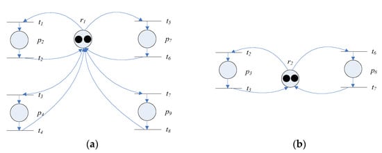
Figure 1.
Examples of , where : (a) (b) .
Definition 3.
A resource subnetfor a type-resource is a discrete timed Petri net= (,,,,) that consists of a number of activities of type-resources, where and the functionis used to specify the firing time of each transition in. Each activity is represented by a circuit [36] in which a number of transitions and places forms a closed loop. A resource subnet has an idle state place denoted by . The set of all idle state places of resources is denoted by = . Without loss of generality, we will also refer to the type- resource by whenever it is clear from the context.
Figure 1a,b show two resource subnets, and . There are four circuits, , , and in . There are two circuits, and in .
Definition 4.
The capacity of type-resources in periodis denoted as, where=for all, whereis the time horizon.
A CPPS may process different types of tasks. Let denote the set of task types. Each task consists of a number of operations. Each operation can be specified by transitions. A type of task is described by a task subnet. Therefore, the task subnet considered in this study consists of a sequence of transitions. Let denote the set of transitions in a task subnet. A transition may involve multiple resources.
Definition 5.
A typetask subnet,, is a discrete timed Petri net which consists of a sequenceoftransitions in the setand a sequence,, ,…,ofplaces in, whereis a function that specifies the lower bound of the firing time of each transition. The first transitionis a fictitious transition that represents the release of a task. The transitionrepresents completion of the final operation of the task. The last transitionis a fictitious transition that represents the removal of a completed task.
Note that the set of transitions in requires allocation of resources, i.e., and . A transition involving multiple resources is characterized by . The number of resources required to fire transition , where , is denoted by .
Figure 2a,b show two task subnets, and .
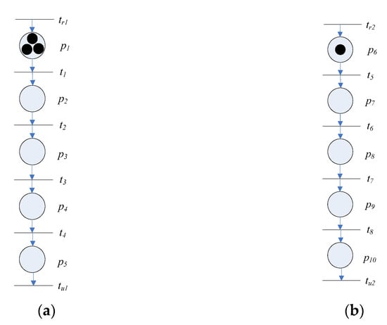
Figure 2.
Examples of , where : (a) ; (b) .
To convey the idea to construct the model, we introduce a composition operator “” to merge two or more DTPN models through common transitions, places and arcs. There are many composition or synthesis methods in the literature (e.g., [13,52,53,54,55]). These include composition by merging transitions or places. Several operations that preserve the liveness property of the composed nets have been proposed in [52,53]. These operations include the fusion of a series of places or transitions and parallel places or transitions, and the elimination of self-loop places or transitions. Some of these studies focus on the synthesis of Petri nets for manufacturing systems (e.g., [13,55]). For this paper, the composition operation is used to capture the synchronization of resources and workflows. Therefore, the composition operation used in this paper is the same as the one used in [13]. It is defined as follows.
Definition 6 ([13]).
Given two discrete timed PNs,= (,,,,) and= (,,,,), the operatorto combineandis defined as follows:
= (,,,,,), where,,,,and.
Although the composition operation is the same as the one in [13], the properties and structure of the resulting models obtained by the composition operation are different from the ones obtained in [13]. The DTPN models considered in this paper allow more complex interactions patterns between resources and tasks. Hence, the liveness property of the composed DTPN models may not be preserved (This point is discussed in Section 4 of this paper). This is the reason why a control policy is needed to maintain the liveness property of the composed DTPN models.
Definition 7.
A nominal model is described by a discrete timed Petri net =, whereand== (,,,,), where. The state ofis called a marking and it is represented by a vector.
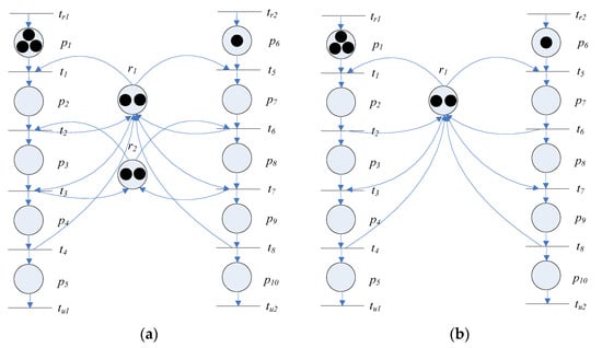
To make it clear for readers to understand the differences between the models used in this paper and the one proposed in [13], we illustrate their differences by an example. Figure 3b is a model that is similar to the one proposed in [13]. Note that the model in Figure 3b only allows at most one resource involved for each transition. By contrast, there are two types of resources involved in transitions , , and in the model of Figure 3a. This is due to the synchronization of operations with the two resources in CPPS. Obviously, this means that the model proposed in this paper allows more complex interactions patterns between resources and tasks. That is, the model proposed in this paper extends the one proposed in [13]. However, this powerful modeling capability should be used in conjunction with a proper control method. Note that the overall model in Figure 3b will not evolve to any undesirable state no matter what sequence of transitions is fired. However, the overall model in Figure 3a may evolve to the circular waiting state in Figure 4. In Figure 4, all resources are held by tasks in the production processes and wait for the resources to be released. Therefore, the development of a method to supervise and control the usage of resources is an important issue.
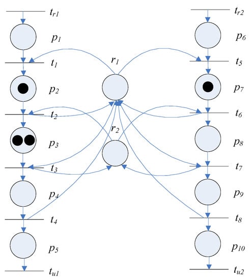
Figure 4.
An undesirable state in which the two types of resources are in a circular waiting situation and a subset of transitions can no longer be fired.
Before defining the control policy, we first define the initial marking and the final marking of the CPPS model. The initial marking is set according to the order requirements. The requirements of an order can be described by product demands, , where and deadline . The initial marking (state) and final marking (state) is defined as follows.
Definition 8.
Suppose the order requirements for type-j tasks is . The number of tokens in the first placeunder the initial markingof the type-j task subnetis, where.
The final marking of the CPPS model is defined as follows.
Definition 9.
For a task subnetin the final statein which the order requirements for type-j tasks is fulfilled, the number of tokens in the last placeof the final marking is.
Definition 10.
Let r denote the idle place of type-r resource subnet. The final state of the type-r resource subnetsatisfies=. That is, resources are in an idle state after processing the required tasks.
Based on the initial states of tasks and resources, we define the CPPS model in the initial state as = , where and = =. Based on the final states of tasks and resources, we define the CPPS model in the final state as = , where and GR = = (PR, TR, FR, , μR).
In the CPPS model , a controlled transition is a transition that requires an allocation of resources to be fired. Let , where , be the set of controlled transitions in . We define a control action as a vector in that specifies the number of times each transition in to be fired concurrently. A sequence of control actions {} is called a control policy . The behaviors of under a control policy is denoted by .
Definition 11.
A CPPS modelunder a control policyis represented by a controlled DTPNand is abbreviated as, whereis a control policy that is defined by a mapping:→that generates a sequence {} of control actions for.
A control action is a vector in that specifies the number of times each transition in to be fired concurrently. Suppose = {, , , , , }. For the marking in Figure 3a, the control action = [2 0 0 0 0 0] can be applied to fire transition twice. A sequence of control actions to be executed in the CPPS model define a control policy. Not all control policies can preserve the liveness property of the system. For the example in Figure 3a, = [2 0 0 0 0 0], = [0 2 0 0 0 0] and = [1 0 0 1 0 0] are three control actions that can be applied consecutively from the marking in Figure 3a. Applying the sequence of control actions , and will fire three times, fire two times and fires one time. The sequence of control actions , and define a control policy. However, this control policy brings the CPPS to an undesirable circular waiting situation in Figure 4. Therefore, generation of the control actions that can maintain the liveness of the CPPS model is an important issue. The Context-Generation Algorithm for CPPS to be introduced in Section 5.3 serves to generate the sequence of control actions to be executed.
When an order is released to CPPS, processing of the order can be represented by the evolution of the states of the model of CPPS under a control policy. The requirements of an order can be described by product demands, , where , and deadline , where the deadline is specified by a period in the time horizon .
In the model of CPPS, a marking represents the state of the system. Before processing the given order, the CPPS is in its initial state with the initial marking . For the given order requirements, the number of different types of products to be produced to fulfill the product demands of the order can be represented by a final marking in the model of CPPS. Whether the order deadline can be met can be calculated by determining whether the marking can be reached from by the deadline . Throughout the evolution from , the CPPS may visit undesirable states. An improper control policy may bring the system to an undesirable state under which some or all the transitions can no longer be fired. Figure 4 shows an example of an undesirable state in which transitions can no longer be fired, with the exception of and . There is a research issue and question that needs to be addressed: can the CPPS model reach the target (final) state by the deadline without visiting any undesirable state? To answer this question, we formulate the Deadline Awareness Problem and the Future States Awareness Problem.
Based on the model of CPPS, we formulate the Deadline Awareness Problem. As the Deadline Awareness Problem is to determine whether the requirements of a given order can be fulfilled by the order deadline, the Deadline Awareness Problem is to determine whether final marking can be reached by the deadline . Formally, this problem can be stated as:
Deadline AwarenessProblem
Given the model of a CPPS with an initial marking , determine whether can be brought to the target marking from by the deadline under some control policy, where and the deadline are specified by the order requirements.
For the target marking and the deadline corresponding to the given order requirements, the Future States Awareness Problem can be formulated as follows.
Future States AwarenessProblem
Given the model of a CPPS with an initial marking , determine whether there exists a control policy to bring to the target marking without visiting any undesirable states, where the marking is the marking corresponding to the given order requirements.
5. Approach to Deadline Awareness Problem and Future States Awareness Problem
To solve the Deadline Awareness Problem and Future States Awareness Problem, we must analyze the evolution of the markings of the CPPS model. We propose an optimization approach to determine a control policy for CPPS. In this section, we first analyze the liveness condition of CPPS in Section 5.1 and Section 5.2 as the liveness property to be defined in Definition 12 is not directly related to the timing aspect. Analysis of the timing or temporal properties of CPPS is presented in Section 5.3 of this paper.
5.1. Analysis of the CPPS Model
Note that the model of a CPPS is an abstraction of the underlying production system. The minimal resource requirements must be satisfied for the CPPS to run and manufacture the products of an order. The minimal resource requirements for the model of a CPPS can be represented by a marking , where .
The Future States Awareness Problem is concerned with whether the target marking can be reached without visiting any undesirable states. In Petri net theory, the concept of liveness property ensures that undesirable states will not be visited. Therefore, we solve the Future States Awareness Problem based on the concept of liveness in Petri nets. We define the liveness of as follows.
Definition 12.
is live if for each marking reached fromunder, each transition can still be fired ultimately by progressing through some further firing sequence.
For the existence of a control policy under which is live, there must be sufficient resources under the initial marking . In this paper, it is assumed that the initial marking satisfies the condition: . Under this assumption, the following property states a liveness condition for the model of a CPPS.
Property 1.
is live under a control policyif and only if there is a sequence of control actions that can bring each markingreached under control policytowith.
Proof.
Sufficiency:
We must prove that if there is a sequence of control actions that can bring each marking reached under control policy to with , is live under the control policy . To show that is live under the control policy , we must show that each transition can still be fired by progressing through some further firing sequence from . Note that . The resources under satisfy the minimal resource requirements. Therefore, we can construct a sequence of control actions to fire transition in type- task subnet by firing sequentially. As the requirements to fire transition in is , the firing sequence can be fired. Therefore, transition can be fired by progressing through the firing sequence .
Let be the marking reached after firing . Under , all the resources return to the idle state. Hence and every transition can be fired again by progressing through some firing sequence again. Based on the above reasoning, each transition can still be fired by progressing through some further firing sequence from .
Therefore, is live under the control policy .
Necessity:
Let be a marking reached under the given control policy . We prove by constructing a firing sequence that can bring to with . We first construct a firing sequence that can bring to under which all the resources are returned to an idle state. As is live under a control policy , for each marking reached from under , each transition can still be fired by progressing through some further firing sequence. There must exist a firing sequence from such that the last transition is fired at least times for each type- task subnet, . We construct a firing sequence based on to complete all the remaining tasks under without introducing new tasks as follows.
Consider a type- task subnet, where . As transition of type- task subnet is fired at least times, firing sequence from can be represented as , where transition appear in exactly times. Note that firing sequence may contain transition and transition may appears a number of times in . This means that transition may also be fired in a number of times. Firing transition will bring new task (s) into type- task subnet and may make the transitions at the downstream fired in . We construct a firing sequence based on by removing transition and all relevant transitions at the downstream of fired in . Removing the transitions of new tasks from reduces the number of resources to be used for firing transitions. As can be fired from , the resulting firing sequence can also be fired from . Note that all the remaining operations in the existing tasks in type- task subnet under will be completed after firing . Therefore, all the resources required by type- task subnet will return to the idle state. In this way, we have constructed a firing sequence that can be fired from .
Note that the firing sequence is still a valid firing sequence that can be fired from and transition of type- task subnet is fired at least times in for each type- task subnet, where . Therefore, we can follow a similar procedure to construct a firing sequence to complete all the remaining operations in the existing tasks in each type- task subnet under for each one by one. After firing from , a marking will be reached and all the resources required by each type of task subnets will return to the idle state under . Due to the conservation of resources, the set of resources in an idle state under is the same as that under , therefore, . As , . Therefore, we have proved that the firing sequence that can bring to with . Let , , …, be the sequence of control actions associated with the firing sequence . Hence, there is a sequence of control actions , , …, that can bring each marking reached under control policy to with .
This completes the proof. □
5.2. An Optimization Approach to Determining a Control Policy for CPPS
Direct application of the existing reachability analysis method to determine the condition of Property 1 about whether there is a sequence of control actions that can bring a marking to with is not feasible as the state space of reachable markings of the CPPS model grows with problem size. The way we work around this problem is to construct a Joint Spatial-Temporal Network (JSTN) to capture the spatial and temporal dynamics of workflows in the networks. Timing information is taken into consideration in constructing the JSTN to capture the spatial and temporal constraints of workflows. The firing time of each transition is used in construction of a JSTN.
Based on JSTN, we will formulate a problem to determine whether there is a sequence of control actions that can bring a marking to with . The algorithm to construct a JSTN is based on Algorithm 1 to construct the Spatial-Temporal Network (STN) for each type of task subnet. Algorithm 1 shows the Spatial–Temporal Network Construction Algorithm for a Type- Task Subnet. The logic of Algorithm 1 to construct a STN for each type of task subnet is highly intuitive. Algorithm 1 first creates a start node and an end node . For a time horizon of periods, Algorithm 1 creates nodes for each , iteratively. Algorithm 1 creates an arc to connect start node to the first node and then create horizontal arcs and non-horizontal arcs, iteratively. Finally, Algorithm 1 creates arcs to connect to the end node . The earliness penalty function for period and the lateness penalty function for are used to set the weight of arcs.
| Algorithm 1: Spatial–Temporal Network Construction Algorithm for Type- Task Subnet |
| Input: , , Output: , where is the set of nodes and is the set of arcs Step 0: Create the start node Create the end node Step 1: For to For each to Create a node with number End For End For Step 2: Create arc from node to the node Set arc cost Step 3: For to For each to Create an arc Set arc cost to 0 End For End For Step 4: For to For each to If Create arc Set arc cost Find the resource type for processing operation , the set of arcs in the spatial–temporal network of type- task involved in the use of type- resource in period End If End For End For Step 5: For each to Create arc from node to node If Set arc cost Else Set arc cost End If End For |
The Joint Spatial–Temporal Network Construction Algorithm in Algorithm 2 first iteratively invokes Algorithm 1 to construct the Spatial-Temporal Network (STN) for each type of task subnet and then construct with and . Algorithm 2 finally merges all start node for all into one source node to obtain the JSTN. Algorithm 2 in shows the Joint Spatial–Temporal Network Construction Algorithm. Note that the structure of a JSTN is different from that of a STN in [10] as JSTN represents the spatial–temporal relation of multiple types of tasks whereas a STN represents only the spatial–temporal relation of a single type of tasks.
Figure 5 shows the structure of a JSTN.
| Algorithm 2: Joint Spatial–Temporal Network Construction Algorithm |
| Input: |
| Task subnets: , |
| Time horizon: , |
| Deadline: |
| Output: Joint Spatial–Temporal Network: , where denotes the set of nodes and denotes the set of arcs |
| For each |
| Construct by applying Algorithm 1, where is the set of nodes and is the set of arcs created. |
| Let be the start node and end node of , respectively. |
| Construct with |
| End For |
| Merge all start node , in into one start node . |
| Return |
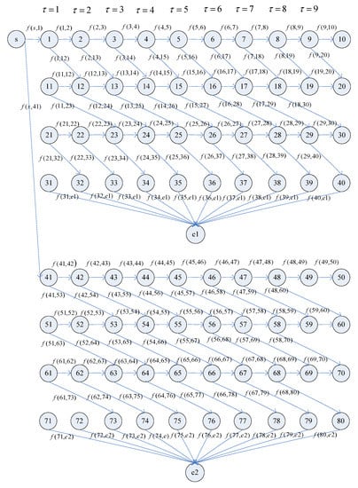
Figure 5.
A Joint Spatial–Temporal Network (JSTN).
The STN of type- task subnet in is denoted as . We define the subset of arcs in that require type- resources in period below.
Definition 13.
is the set of arcs requiring the type-resources in period .
Note that the states across the time horizon of the CPPS model can be represented in the corresponding STNs. Therefore, we propose an optimization problem formulation to determine whether there exists a control policy that can bring to without visiting undesirable states by the deadline.
The following Nominal Optimization Problem (NOP) is formulated based on the Joint Spatial–Temporal Network to find a solution. The NOP aims to complete the production activities for the given order by the deadline. Therefore, the objective function is the overdue cost described in (1) under the capacity constraints of different types of resources in (2), the flow balance constraints in (3), the product requirements of the order in (4), (5) and the decision variables must be nonnegative integers as described in (6).
Nominal Optimization Problem (NOP) based on the Joint Spatial–Temporal Network
where is the set of nonnegative integers.
A solution of NOP can be used to define the control actions to bring from to without visiting undesirable states. Whether the deadline can be met depends on the solution found for NOP. Theorem 1 states a condition for ensuring the liveness of . In the proof of this theorem, we first define the control actions based on a solution of NOP. We then prove that the control actions will bring from to without visiting undesirable states.
Theorem 1.
There exists a solution to the Nominal Optimization Problem if and only if there exists a control policy under whichis live and can reachunder.
Proof.
Proof of “only if part”:
We prove by constructing a control policy under which is live given the precondition that there exists a solution to NOP. To construct a control policy under which is live, we first define the control actions for the given solution based on the following definitions of control actions. The set of arcs in STN can be divided into three subsets, , the set of arcs corresponding to waiting states, , the set of arcs corresponding to busy (processing) states. There is a transition corresponding to an arc . Suppose the time horizon is divided into period. Let denote the set of time period. A control action for time period is denoted by and denotes the control action to be applied to transition in period . For each arc , , starting with period , let be the transition associated with arc . We define the control action , which will be applied to fire transition corresponding to an arc in period for times. These control actions , , define a control policy associated with the solution . Based on the above definitions, we show that the control actions , defined above can be executed. That is, for each , can be fired times in period . We prove by showing that under the marking reached after applying the control actions , , ,…, , there exists a control policy under which is live.
For = 1, we prove that the control action applied to all relevant transitions in period 1 can be executed. Note that the number of type- resources required to fire transitions in type- subnet in period 1 is . The total number of type- resources required to fire transitions in type- subnet in period 1 is , which is equal to . The total number of type- resources required to fire transitions in type- subnet in period 1 is . As constraint (2) holds for each and each period , is greater than or equal to and is equal to , all relevant transitions allowed to be fired under control action can be executed in period 1. Similarly, for period = 2, the number of type- resources required to fire transitions in type- subnet in period 2 is , which is equal to . The total number of type- resources required to fire transitions in type- subnet in period 2 is , which is equal to . As is greater than or equal to and is equal to , is greater than or equal to . All relevant transitions under control action can be executed in period 2.
As the above reasoning holds for all , the sequence of control actions , , can be executed. After executing all these control actions, the final marking will be reached. Under , all resources are returned to an idle state. Hence, the set of resources is the same as . As , .
Proof of “if part”:
If there is a control policy under which is live and can reach under , we need to show that there exists a solution to the Nominal Optimization Problem.
If is live under a control policy , the initial marking must satisfy the minimal resource requirements: and there must be sufficient resources to fire the transitions in each type of task subnets separately. We construct a sequence of control actions to bring from to as follows. First, we construct a sequence of control actions to bring from to under which the number of tokens in the last place of type-1 subnet is . Let , , …, be the sequence of control actions that repeatedly fire transitions in sequentially for times from . At period , the number of tokens in the last place of type-1 subnet is and all the resource tokens are returned to an idle state. Therefore, under the set of resources n idle state is the same as the set of resources under . Then, we construct a sequence of control actions , , …, to bring from to under which the number of tokens in the last place of type-2 subnet is and the number of tokens in the last place of type-1 subnet is . All the resource tokens are returned to an idle state under . Therefore, under the set of resources n idle state is the same as the set of resources under . By following a similar procedure, we can construct a sequence of control actions , , …, , , , …, , …, , , …, to bring from to under which the number of tokens in the last place of type- subnet is and all the resources are returned to an idle state.
As all resources are returned to an idle state under, , the sequence of control actions , , …, , , , …, , …, , , …, brings from to . As is a solution of the Nominal Optimization Problem, conservation of flows due to constraints (3), (4) and (5) must be satisfied. Therefore, = . So can be reached after executing the sequence of control actions , , …, , , , …, , …, , , …, . The sequence of control actions , , …, , , , …, , …, , , …, is a control policy to reach .
This completes the proof. □
5.3. Situation-Aware Context Generation Algorithm
In this subsection, we first present Theorem 2 for deadline awareness and future states awareness and then a context generation algorithm for CPPS. Based on Theorem 1, we have the following result.
Theorem 2.
Assume that= 0 forandfor. If there exists a solution to the Nominal Optimization Problem, there exists a control policy under whichcan reachwithout visiting any undesirable states. If the objective function value of the solution to the Nominal Optimization Problem is zero, can reachby the deadlineunder control policy.
Proof.
Let be a solution to the NOP. It follows from Theorem 1 that there exists a control policy under which is live and can reach under . Hence, undesirable states will not be visited under . If the objective function value of the solution to the Nominal Optimization Problem is zero, must be 0.
Let denote the set of arcs in the type-j task subnet directly connecting to the end node . Note that each term in can be broken down into two terms, and .
As is equal to zero for all arcs with the exception of the arcs that connect to the end nodes, the following holds:
= 0 for each .
Therefore, the term is reduced to , which is equal to .
As = 0 for , is equal to zero for each and is reduced to .
Hence is equal to 0.
As for, > 0 for each .
As is nonnegative, must be zero for each .
Therefore, the deadline can be met. □
Based on the theorem presented above, we propose Algorithm 3 to generate the contextual information (control actions) for Future States-Aware systems. The following algorithm first constructs for the model of a CPPS with an initial marking and formulates NOP next. Finally, the NOP is solved to find a solution. If a solution can be found by solving the NOP, the proposed algorithm will generate the Future States-Aware Context. Otherwise, it will exit.
| Algorithm 3: Context Generation Algorithm for CPPS |
| Step 1: Construct for the model of a CPPS with an initial marking |
| Step 2: Formulate the nominal optimization problem |
| Formulate NOP according to |
| Step 3: Solve the nominal optimization problem |
| Find the solution of NOP |
| If there is a solution |
| if = 0 |
| The deadline can be met. |
| Else |
| The deadline cannot be met. |
| End If |
| Go to Step 4 |
| Else |
| Exit |
| End If |
| Step 4: Construct the control actions based on the solution found |
| For |
| For each |
| For each |
| Find the arc associated with transition and period |
| End For |
| End For |
| End For |
In Property 2, we analyze the complexity of constructing the Joint Spatial-Temporal Network.
Property 2.
The complexity of constructing the Joint Spatial-Temporal Networkby applying the Joint Spatial–Temporal Network Construction Algorithm is.
Proof.
As a CPPS consists of a number of task subnets, the Joint Spatial–Temporal Network Construction Algorithm constructs by applying Algorithm 1 to construct . As the number of transitions in different task subnets may not be the same, to analyze the complexity of constructing , let denote the number of transitions in the task subnet with the maximum number of transitions. The number operations to create nodes in is less than or equal to for each . The number operations to create arcs in is less than or equal to for each . Hence, the total number of operations to create is less than or equal to . As there are types of task subnets, the total number of operations to create for each is less than or equal to . The number of operations to merge all start nodes is and the number of operations to merge all start nodes is . Therefore, the total number of operations to construct is less than or equal to . Therefore, the complexity of constructing is . □
We establish a lower bound on the complexity of solving NOP in Property 3.
Property 3.
A lower bound on the complexity of solving NOP is.
Proof.
As the Nominal Optimization Problem is formulated based on the Joint Spatial–Temporal Network, it is similar to the classical minimum cost flow problem in the literature as the flow balance constraints must be satisfied. However, the Nominal Optimization Problem is different from the classical minimum cost flow problem in that the additional capacity constraints must be satisfied. Therefore, the complexity of solving the Nominal Optimization Problem is expected to be different from that of the classical minimum cost flow problem. Despite this difference, the complexity of the classical minimum cost flow problem provides a lower bound on the complexity of the Nominal Optimization Problem. As the number of nodes in the Joint Spatial–Temporal Network is proportional to , . □
6. Results
The theory and algorithm presented in the previous sections are illustrated by a small example. In addition, we conducted a series of experiments to assess the computational efficiency of the proposed methods and to illustrate the potential to solve real problems. The test data for the small example is described in details in the text. The test data for large examples can be downloaded from the following link:
https://drive.google.com/drive/folders/1SCcf-VWkrSy_iwUoUw0Ky-xxZCrdKtBo?usp=sharing (accessed on 27 February 2021).
All the experiments were conducted on a personal computer with Intel CoreTM i7-4720 HQ CPU, 2.6 G Hz, and 16 GB of onboard memory.
6.1. An Example
In this subsection, we illustrate the proposed method with an example.
Example 1.
Consider a CPPS with two production processes to produce two types of products. The two production processes are modeled by two task subnets. There are two types of resources in the CPPS. The two task subnets share the two types of resources. The model of the CPPS is depicted in Figure 3a. The firing time of each transition is listed in Table 2. Suppose an order is received and is to be released to the CPPS for processing the products. The requirements of the order are shown in Table 3. The product demands of the order include three type-1 products and one type-2 product. The deadline of the order is the eighth period. For this example,, = 3,= 1,, . We set the time horizon. Therefore,=and=. The nominal capacity of type-resources in periodis= 2 for eachand. The total number of type-resources in each periodis listed in Table 4. The initial marking=for. In this example, we use set the function= 0 forandforto penalize overdue. As, , andfor all the other arc. For this example,is listed in Table 5.
Table 2.
Firing time of each transition in Figure 3a.
Table 3.
Requirements of an order.
Table 4.
The nominal capacity of each type of resources in each period.
Table 5.
The data of .
The NOP for this example is as follows, where (7) is the objective function, (8) is the capacity constraints, (9) is the flow balance constraints, (10), (11) are the demand constraints, (12) and (13) are the final product constraints.
where is the set of nonnegative integers.
We apply the CPLEX problem solver [56] to solve the NOP in the Context-Generation Algorithm. By solving the NOP, we find the solution in Table 6, which can be represented in the Joint Spatial-Temporal Network in Figure 6. The objective function value is 0. Therefore, the deadline can be met.
Table 6.
The solution obtained by solving NOP.
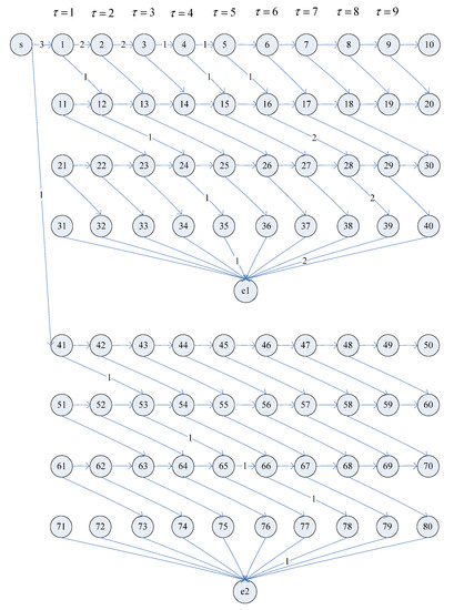
Figure 6.
A solution of NOP represented in JSTN.
Table 7.
The sequence of control actions.
Following is an explanation of the control actions generated for the first period and the second period. For the first period ( = 1), the control action = [1 0 0 1 0 0] represents that transition and transition will be fired. This means that the two transitions will be fired concurrently. For the second period ( = 2), the control action = [0 1 0 0 0 0] represents that transition will be fired. Note that all the constraints are satisfied for the generated control actions.
6.2. Computational Experience
In this section, we study how the CPU time grows with the scale of the problems. The data of test cases (Problem 1 through Problem 15) are available for downloading from the following link:
https://drive.google.com/drive/folders/1SCcf-VWkrSy_iwUoUw0Ky-xxZCrdKtBo?usp=sharing (accessed on 27 February 2021).
In CPPS, the problem size parameters include the maximal number of operations in the task subnets, the time horizon and the number of task types. These problem size parameters correspond to the parameters , and in this paper. To study the influence of each parameter on the CPU time, we perform many experiments by changing each parameter and recording the results. We illustrate the consistency between the results and our expectations.
First, we perform several experiments by changing the parameter from 10 to 50 while keeping other parameters unchanged ( = 4 and = 200). To be specific, we set to be 10, 20, 30, 40 and 50, respectively. The results are shown in Figure 7. The results indicate that the CPU time grows approximately linearly with . This result is better than the projection of the polynomial lower bound on the complexity of solving NOP.
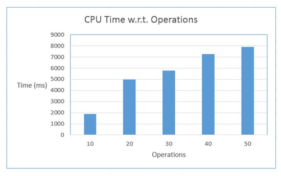
Figure 7.
CPU time with respect to the number of operations (Problems 1~5).
To study the growth of CPU time with respect to the time horizon, we perform several experiments by changing the parameter from 100 to 500 while keeping other parameters unchanged (= 4 and = 10). To be specific, we set to be 100, 200, 300, 400 and 500, respectively. The results are shown in Figure 8. The results indicate that the CPU time grows polynominally with . This result is consistent with the projection of polynomial lower bound on the complexity of solving NOP.
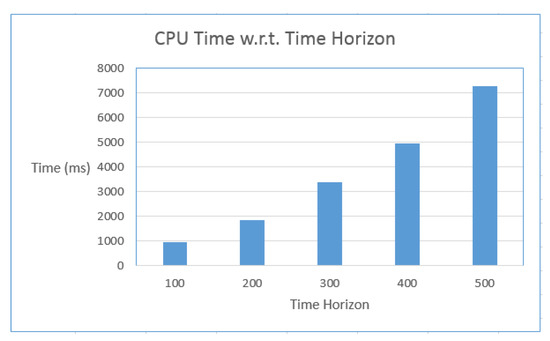
Figure 8.
CPU time with respect to time horizon (Problems 11~15).
To study the growth of CPU time with regards to the number of task types, we perform several experiments by changing the parameter from 4 to 20 while keeping other parameters unchanged ( = 100 and = 10). To be specific, we set to be 4, 8, 12, 16 and 20, respectively. The results are shown in Figure 9. The results indicate that the CPU time grows polynominally with . This result is consistent with the projection of polynomial lower bound on the complexity of solving NOP.
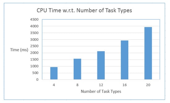
Figure 9.
CPU time with respect to number of task types (Problems 21~25).
7. Discussion
In this paper, we propose the theory to lay a foundation for developing context-aware applications in CPPS. Two context awareness properties are crucial for the development of context-aware applications in CPPS. One is deadline awareness and the other is future states awareness. We develop a theory to pave the way for deadline-aware and future states-aware applications in CPPS based on Discrete Timed Petri Nets. The theory and algorithms developed in this paper provide an approach to determining whether the deadline of an order can be met without visiting any undesirable states. Accompanying the theory presented in this paper is an example to illustrate the application of the theory.
As computational feasibility is an important factor in the development of context-aware applications for CPPS, analysis of computational complexity and verification by experiments are important steps to illustrate the practicality of the theory for solving real problems. Therefore, we conduct an analysis of the decision problem and conduct experiments to study the computational feasibility of the proposed method. We study how the CPU time grows with the scale of the problem. In CPPS, the problem size parameters include the maximal number of operations in the task subnets, the time horizon and the number of task types. These problem size parameters correspond to the parameters , and in this paper.
The algorithm to construct JSTN is of polynomial complexity (according to Property 2: The complexity to construct the Joint Spatial–Temporal Network by applying the Joint Spatial–Temporal Network Construction Algorithm is . A lower bound on the complexity of solving NOP, which is defined on JSTN, is according to Property 3. Overall, a lower bound on the complexity of constructing JSTN and solving NOP is of polynomial complexity.
To study the influence of each parameter on the CPU time, we perform many experiments by changing each parameter and recording the results. Our experimental results show that the CPU time grows approximately linearly with and grows polynominally with and . These results are consistent with the projection of the polynomial lower bound on the complexity of solving NOP. Based on our experimental results, we illustrate the consistency between the results and our expectations. This also indicates the practicality of the proposed theory in solving real problems in CPPS. Figure 7 through Figure 9 includes the construction of JSTN and solving of NOP. Note that markings of CPPS are neither embedded nor included in the construction process of JSTN. This avoids the state explosion problem.
In the literature, different approaches were proposed to tackle the complexity issue of time Petri nets and timed Petri nets. Berthomieu et al. [46,47,48] and Klai et al. [49] proposed different methods to reduce complexity in the analysis of time Petri nets. Lefebvre et al. proposed different methods to reduce complexity in the analysis of time Petri nets [50,51]. In terms of the models used, the nets considered by all the works mentioned above were general, whereas a subclass of nets is considered in our paper. Even though only a subclass of nets is considered, the subclass of nets considered in this paper can be used to model the production processes commonly used in the manufacturing sector. As the net structure considered in the works mentioned above is general, a variety of approaches such as the construction of a State Class Graph, Timed Aggregate Graph, Timed Extended Reachability Graph and Approximated Timed Reachability Graph were proposed to reduce complexity. However, all these methods suffer from state explosion problems as the complexity of constructing and exploring variants of reachability graphs grows exponentially with the problem size. As the models used in this paper belong to a subclass of nets, we developed a more efficient algorithm based on the proposed JSTN based method by exploiting the net structure. The proposed JSTN based method does not rely on the explicit construction of reachability graphs, State Class Graphs or Timed Extended Reachability Graphs or their variants. As a result, we can identify a lower bound on the complexity of constructing JSTN and solving NOP, which is of polynomial complexity.
The problems addressed in this study are different from the ones in the literature. Although there are many approaches to context-aware workflow systems in [57], there are only a few studies on the development of context-aware applications and services based on different variants of Petri nets, e.g., [58,59,60]. In particular, existing studies on modeling, analyzing and generating time-relevant contextual information for context-aware applications and systems are limited, e.g., [9,13,15,61]. Issues regarding the achievement of situation awareness, including deadline awareness and future states awareness in Cyber-Physical Production Systems is less explored. This paper attempts to bridge this gap by expanding the preliminary results reported in [62] through developing relevant theory and algorithms to address situation awareness problems of CPPS, and conducting experiments to study the feasibility of the proposed approach. The results of this study confirm the feasibility of the proposed method.
8. Conclusions
The complex workflows and heterogeneous entities in CPPS pose several challenges in the development of context-aware applications for CPPS. Due to contention and sharing of resources among different workflows and production processes in CPPS, a state that is seemingly not undesirable at one point in time may evolve to another state that is undesirable in the future. Therefore, development of context-aware applications for CPPS should consider not only the current state but also future states of the system. In other words, situation awareness is an important factor that must be considered in context-aware applications for CPPS. However, relevant studies are still lacking on situation awareness for CPPS. This situation awareness requirement raises an important research issue in CPPS. For this reason, we focus on the development of a theory for the analysis of situation awareness property for CPPS to pave the way for the development of context-aware applications for CPPS. In this paper, we study problems relevant to identifying situations of CPPS. These include the Deadline Awareness Problem and Future States Awareness Problem. The Deadline Awareness Problem aims to determine whether the deadline can be met in the future, whereas the Future States Awareness Problem aims to determine whether the undesirable states can be avoided in the process to evolve to the target state from the current state in CPPS. We develop the theory and relevant algorithms to address the above problems and support analysis of the situation of CPPS. We illustrate the application of the theory to an application scenario through the use of an example. To assess the computational efficiency of the proposed algorithms, we analyze the complexity and conduct experiments to verify the CPU time for applying the proposed algorithm to many test cases. The results show that the CPU time grows polynominally with the scale of the problem and are consistent with the expected lower bound of computational complexity. This study provides an alternative approach to the analysis of a class of timed Petri nets without relying on the exploration of graphs that are defined in the literature based on the State Class of general time Petri nets, such as the State Class Graph, Timed Aggregate Graph, Timed Extended Reachability Graph and Approximated Timed Reachability Graph. This study sheds light on a promising approach to the development of efficient algorithms for analyzing subclasses of Petri nets by exploiting their structures. The development of relevant theory to analyze situation awareness properties in other problem domains is one interesting direction of future research.
Funding
This research was supported in part by the Ministry of Science and Technology, Taiwan, under Grant MOST 110-2410-H-324-001.
Institutional Review Board Statement
Not applicable.
Informed Consent Statement
Not applicable.
Data Availability Statement
Data available in a publicly accessible repository described in the article.
Conflicts of Interest
The author declares no conflict of interest.
References
- Lee, E.A. Cyber-physical systems-are computing foundations adequate? In Proceedings of the Position Paper for NSF Workshop Cyber-Physical Systems: Research Motivation, Techniques and Road Map, Austin, TX, USA, 16–17 October 2006.
- Ivanov, R.; Weimer, J.; Lee, I. Towards Context-Aware Cyber-Physical Systems. In Proceedings of the 2018 IEEE Workshop on Monitoring and Testing of Cyber-Physical Systems (MT-CPS), Porto, Portugal, 10–13 April 2018; pp. 10–11. [Google Scholar]
- Sahlab, N.; Jazdi, N.; Weyrich, M. An Approach for Context-Aware Cyber-Physical Automation Systems. IFAC-PapersOnLine 2021, 54, 171–176. [Google Scholar] [CrossRef]
- Monostori, L. Cyber-physical Production Systems: Roots, Expectations and R&D Challenges. Procedia CIRP 2014, 17, 9–13. [Google Scholar]
- Lee, J.; Bagheri, B.; Kao, H.-A. A Cyber-Physical Systems architecture for Industry 4.0-based manufacturing systems. Manuf. Lett. 2015, 3, 18–23. [Google Scholar] [CrossRef]
- Cardin, O. Classification of cyber-physical production systems applications: Proposition of an analysis framework. Comput. Ind. 2019, 104, 11–21. [Google Scholar] [CrossRef] [Green Version]
- Hong, J.; Suh, E.; Kim, S.J. Context-aware systems: A literature review and classification. Expert Syst. Appl. 2009, 36, 8509–8522. [Google Scholar] [CrossRef]
- Situation Awareness. Available online: https://en.wikipedia.org/wiki/Situation_awareness (accessed on 28 February 2022).
- Hsieh, F.-S. A Dynamic Context-Aware Workflow Management Scheme for Cyber-Physical Systems Based on Multi-Agent System Architecture. Appl. Sci. 2021, 11, 2030. [Google Scholar] [CrossRef]
- Petri, C.A. Kommunikation mit Automaten. Ph.D. Thesis, Institut für Instrumentelle Mathematik, Bonn, Germany, 1962. [Google Scholar]
- Ramchandani, C. Analysis of Asvnchronous Concurrent Systems by Timed Petri Nets. Ph.D. Thesis, Massachusetts Institute of Technology, Cambridge, MA, USA, 1974. [Google Scholar]
- Merlin, P.M. A Study of the Recoverability of Computing Systems. Ph.D. Thesis, Department of Information and Computer Science, University of California, Irvine, CA, USA, 1974. [Google Scholar]
- Hsieh, F.-S. Temporal Analysis of Influence of Resource Failures on Cyber-Physical Systems Based on Discrete Timed Petri Nets. Appl. Sci. 2021, 11, 6469. [Google Scholar] [CrossRef]
- Lefebvre, D.; Daoui, C. Control Design for Bounded Partially Controlled TPNs Using Timed Extended Reachability Graphs and MDP. IEEE Trans. Syst. Man Cybern. Syst. 2020, 50, 2273–2283. [Google Scholar] [CrossRef]
- Hsieh, F.-S.; Lin, J.B. Development of context-aware workflow systems based on Petri Net Markup Language. Comput. Stand. Interfaces 2014, 36, 672–685. [Google Scholar] [CrossRef]
- Hsieh, F.-S.; Lin, J.-B. Context-aware workflow management for virtual enterprises based on coordination of agents. J. Intell. Manuf. 2012, 25, 393–412. [Google Scholar] [CrossRef]
- Jyotish, N.K.; Singh, L.K.; Kumar, C. A state-of-the-art review on performance measurement petri net models for safety critical systems of NPP. Ann. Nucl. Energy 2022, 165, 108635. [Google Scholar] [CrossRef]
- Riahi, I.; Moussa, F. A formal approach for modeling context-aware Human-Computer System. Comput. Electr. Eng. 2015, 44, 241–261. [Google Scholar] [CrossRef]
- Jyotish, N.K.; Singh, L.K.; Kumar, C.; Ahmed, F.D.; Majid, M.A. Towards agent-based petri net decision making modelling for cloud service composition: A literature survey. J. Netw. Comput. Appl. 2019, 130, 14–38. [Google Scholar]
- Schilit, B.; Adams, N.; Want, R. Context-Aware Computing Applications. In Proceedings of the 1994 First Workshop on Mobile Computing Systems and Applications, Santa Cruz, CA, USA, 8–9 December 1994; pp. 85–90. [Google Scholar]
- Alegre, U.; Augusto, J.C.; Clark, T. Engineering context-aware systems and applications: A survey. J. Syst. Softw. 2016, 117, 55–83. [Google Scholar] [CrossRef]
- Perera, C.; Zaslavsky, A.B.; Christen, P.; Georgakopoulos, D. Context Aware Computing for The Internet of Things: A Survey. IEEE Commun. Surv. Tutor. 2014, 16, 414–454. [Google Scholar] [CrossRef] [Green Version]
- Dey, A.K. Understanding and Using Context. Pers. Ubiquitous Comput. 2015, 1, 4–7. [Google Scholar] [CrossRef]
- Subbu, K.P.; Vasilakos, A.V. Big Data for Context Aware Computing–Perspectives and Challenges. Big Data Res. 2017, 10, 33–43. [Google Scholar] [CrossRef]
- Capurso, N.; Mei, B.; Song, T.; Cheng, X.; Yu, J. A survey on key fields of context awareness for mobile devices. J. Netw. Comput. Appl. 2018, 118, 44–60. [Google Scholar] [CrossRef]
- Kurniawan, I.F.; Asyhari, A.T.; He, F.; Liu, Y. Mobile computing and communications-driven fog-assisted disaster evacuation techniques for context-aware guidance support: A survey. Comput. Commun. 2021, 179, 195–216. [Google Scholar] [CrossRef]
- Kulkarni, S.; Rodd, S.F. Context Aware Recommendation Systems: A review of the state of the art techniques. Comput. Sci. Rev. 2020, 37, 100255. [Google Scholar] [CrossRef]
- Islam, M.S.U.; Kumar, A.; Hu, Y.-C. Context-aware scheduling in Fog computing: A survey, taxonomy, challenges and future directions. J. Netw. Comput. Appl. 2021, 180, 103008. [Google Scholar] [CrossRef]
- Camargo-Henríquez, I.; Silva, A. An Activity Theory-Based Approach for Context Analysis, Design and Evolution. Appl. Sci. 2022, 12, 920. [Google Scholar] [CrossRef]
- Awareness. Available online: https://en.wikipedia.org/wiki/Awareness (accessed on 28 February 2022).
- Napoleone, A.; Macchi, M.; Pozzetti, A. A review on the characteristics of cyber-physical systems for the future smart factories. J. Manuf. Syst. 2020, 54, 305–335. [Google Scholar] [CrossRef]
- Harrison, R.; Vera, D.; Ahmad, B. Engineering Methods and Tools for Cyber–Physical Automation Systems. Proc. IEEE 2016, 104, 973–985. [Google Scholar] [CrossRef] [Green Version]
- Model Driven Architecture. Available online: https://www.omg.org/mda/index.htm (accessed on 28 February 2022).
- The Unified Modeling Language. Available online: https://www.uml.org/ (accessed on 28 February 2022).
- Thramboulidis, K.C. Using UML in control and automation: A model driven approach. In Proceedings of the 2nd IEEE International Conference on Industrial Informatics, Berlin, Germany, 24–26 June 2004; pp. 587–593. [Google Scholar]
- The Systems Modeling Language. Available online: https://sysml.org/ (accessed on 28 February 2022).
- Shah, A.A.; Kerzhner, A.A.; Schaefer, D.; Paredis, C.J. Multi-view modeling to support embedded systems engineering in SysML. In Graph Transformations and Model-Driven Engineering; Springer: New York, NY, USA, 2010; pp. 580–601. [Google Scholar]
- Cao, Y.; Liu, Y.; Paredis, C.J. System-level model integration of design and simulation for mechatronic systems based on SysML. Mechatronics 2011, 21, 1063–1075. [Google Scholar] [CrossRef]
- Petri Net. Available online: https://en.wikipedia.org/wiki/Petri_net (accessed on 28 February 2022).
- Murata, T. Petri nets: Properties, analysis and applications. Proc. IEEE. 1989, 77, 541–580. [Google Scholar] [CrossRef]
- Zuberek, W.M. Timed Petri nets definitions, properties, and applications. Microelectron. Reliab. 1991, 31, 627–644. [Google Scholar] [CrossRef]
- Zuberek, W.M. Timed Petri nets and preliminary performance evaluation. In Proceedings of the 7th Annuual Symposium on Computer Architecture, La Baule, France, 6–8 May 1980; pp. 88–96. [Google Scholar]
- Sifakis, J. Petri nets for performance evaluation. Measuring Modelling and Evaluating Computer Systems. In Proceedings of the 3rd International Symposium IFIP Working Group 7.3, Bonn, Germany, 3–5 October 1977; pp. 75–93. [Google Scholar]
- Marsan, M.A.; Balbo, G.; Conte, G. A class of generalised stochastic Petri nets for the performance evaluation of multiprocessor systems. ACM Trans. Comput. Syst. 1984, 2, 198–199. [Google Scholar]
- Molloy, M.K. Discrete Time Stochastic Petri Nets. IEEE Trans. Softw. Eng. 1985, 11, 417–423. [Google Scholar] [CrossRef]
- Berthomieu, B.; Menasche, M. An Enumerative Approach for Analyzing Time Petri Nets. In Proceedings of the IFIP 9th World Computer Congress, Paris, France, 19–23 September 1983; pp. 41–46. [Google Scholar]
- Berthomieu, B.; Diaz, M. Modeling and verification of time dependent systems using time Petri nets. IEEE Trans. Softw. Eng. 1991, 17, 259–273. [Google Scholar] [CrossRef]
- Berthomieu, B.; Vernadat, F. State Class Constructions for Branching Analysis of Time Petri Nets. In Tools and Algorithms for the Construction and Analysis of Systems; TACAS 2003. Lecture Notes in Computer Science; Garavel, H., Hatcliff, J., Eds.; Springer: Berlin/Heidelberg, Germany, 2003; Volume 2619, pp. 442–457. [Google Scholar]
- Klai, K.; Aber, N.; Petrucci, L. A New Approach to Abstract Reachability State Space of Time Petri Nets. In Proceedings of the 2013 20th International Symposium on Temporal Representation and Reasoning, Pensacola, FL, USA, 26–28 September 2013; pp. 117–124. [Google Scholar]
- Lefebvre, D. A Timed Extended Reachability Graph for the simulation and analysis of bounded TPNs. In Proceedings of the European Simulation and Modelling Conference, Lisbon, Portugal, 25–27 October 2017; pp. 33–37. [Google Scholar]
- Lefebvre, D. Approximated Timed Reachability Graphs for the robust control of discrete event systems. Discret. Event Dyn. Syst. 2019, 29, 31–56. [Google Scholar] [CrossRef]
- Esparza, J.; Silva, M. Compositional synthesis of live and bounded free choice Petri nets. Lect. Notes Comput. Sci. 1991, 527, 172–187. [Google Scholar]
- Murata, T.; Koh, J. Reduction and expansion of live and safe marked graphs. IEEE Trans. Circuits Syst. 1980, 27, 68–71. [Google Scholar] [CrossRef]
- Marechal, A.; Buchs, D. Generalizing the Compositions of Petri Nets Modules, Application and Theory of Petri Nets and Concurrency. Fundam. Inform. 2015, 137, 87–116. [Google Scholar] [CrossRef]
- Jeng, M.D.; DiCesare, F. A review of synthesis techniques for Petri nets with applications to automated manufacturing systems. IEEE Trans. Syst. Man Cybern. 1993, 23, 301–312. [Google Scholar] [CrossRef]
- CPLEX Optimizer. Available online: https://www.ibm.com/analytics/cplex-optimizer (accessed on 28 February 2022).
- Boutamina, S.; Maamri, R. A survey on context-aware workflow systems. In Proceedings of the International Conference on Intelligent Information Processing, Security and Advanced Communication, Batna, Algeria, 23–25 November 2015; pp. 1–6. [Google Scholar]
- Kwon, O.B. Modeling and generating context-aware agent-based applications with amended colored Petri nets. Expert Syst. Appl. 2004, 27, 609–621. [Google Scholar] [CrossRef]
- Hu, Z.; Lu, T.; Zhao, Z. Context-aware service system modeling using timed CPN. In Proceedings of the 2013 10th International Conference on Service Systems and Service Management, Hong Kong, China, 17–19 July 2013; pp. 164–169. [Google Scholar]
- Xing, Z.; Hong, Z.; Yulong, L. A Petri-Net Based Context-Aware Workflow System for Smart Home. In Proceedings of the 2012 IEEE International Symposium on Parallel & Distributed Processing, Workshops and Phd Forum, Shanghai, China, 21–25 May 2012; pp. 2336–2342. [Google Scholar]
- Han, S.; Youn, H.Y. Modeling and Analysis of Time-Critical Context-Aware Service Using Extended Interval Timed Colored Petri Nets. IEEE Trans. Syst. Man Cybern.—Part A Syst. Hum. 2012, 42, 630–640. [Google Scholar] [CrossRef]
- Hsieh, F.S. Robust Supervisory Control for Cyber-Physical Systems based on Discrete Timed Petri nets. In Proceedings of the 2022 IEEE 12th Annual Computing and Communication Workshop and Conference (CCWC), Virtual Conference, 26–29 January 2022. [Google Scholar]
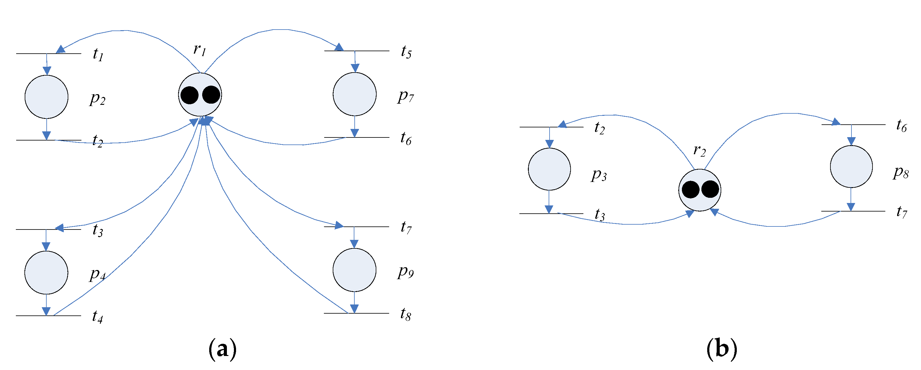
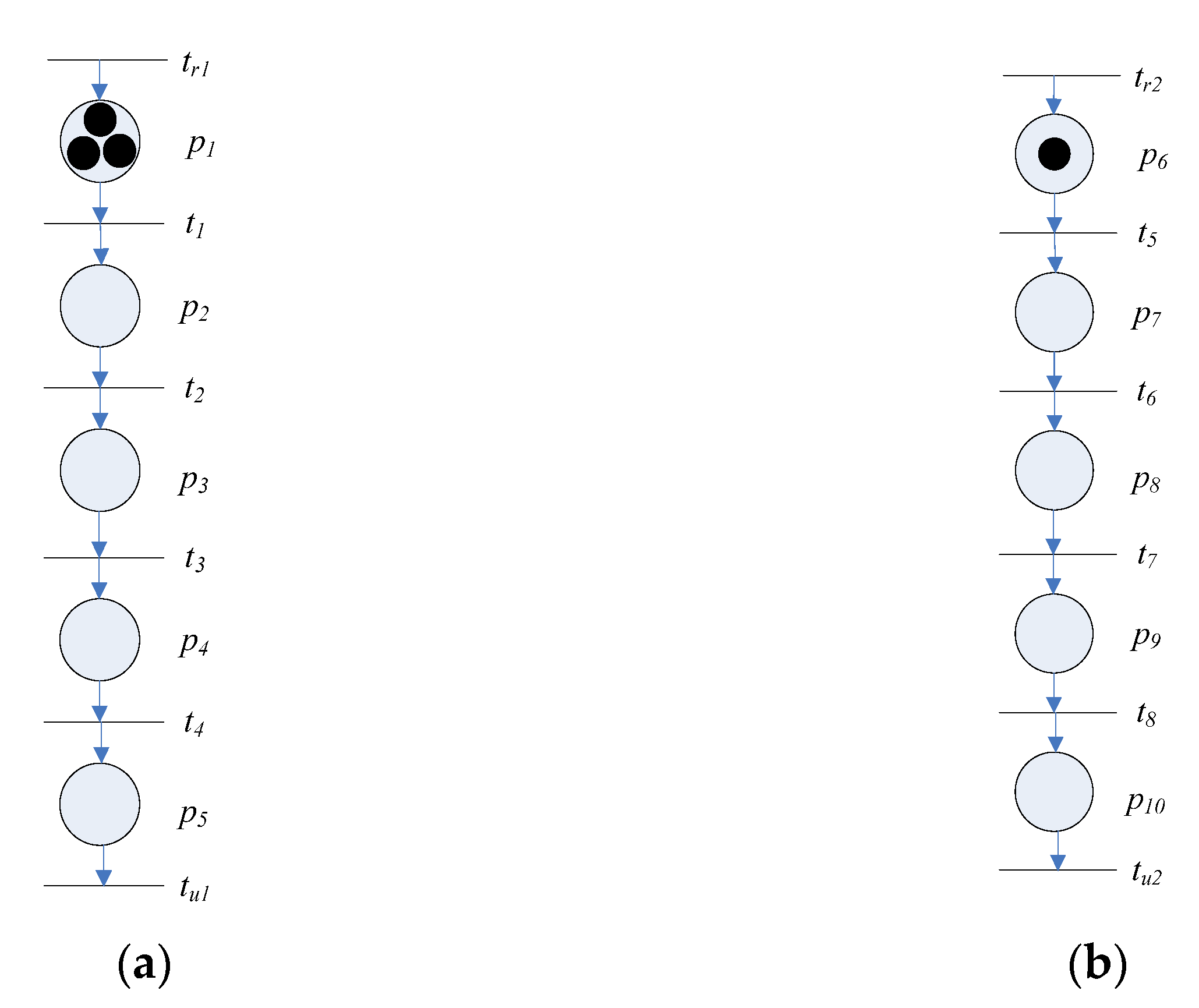
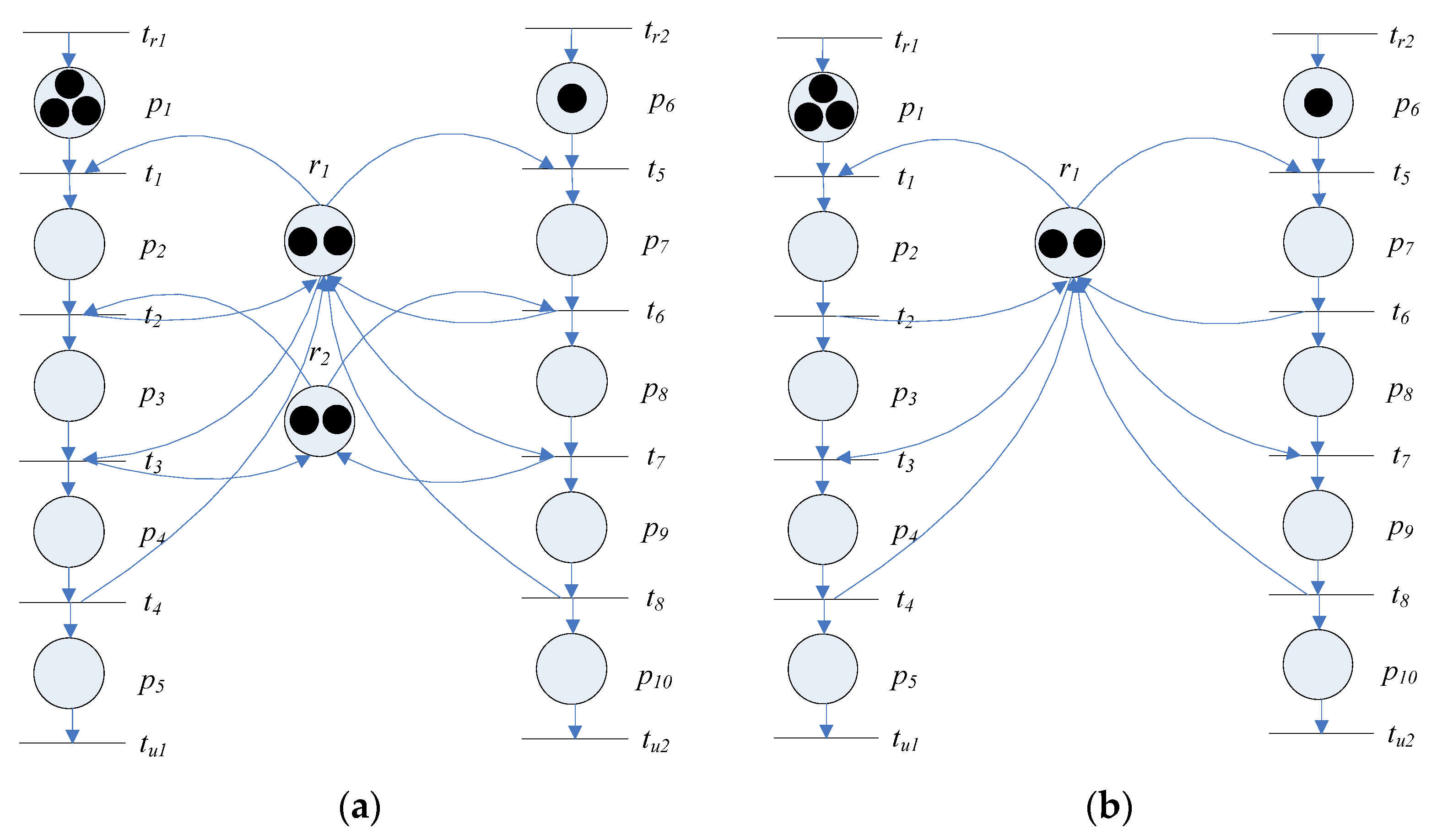
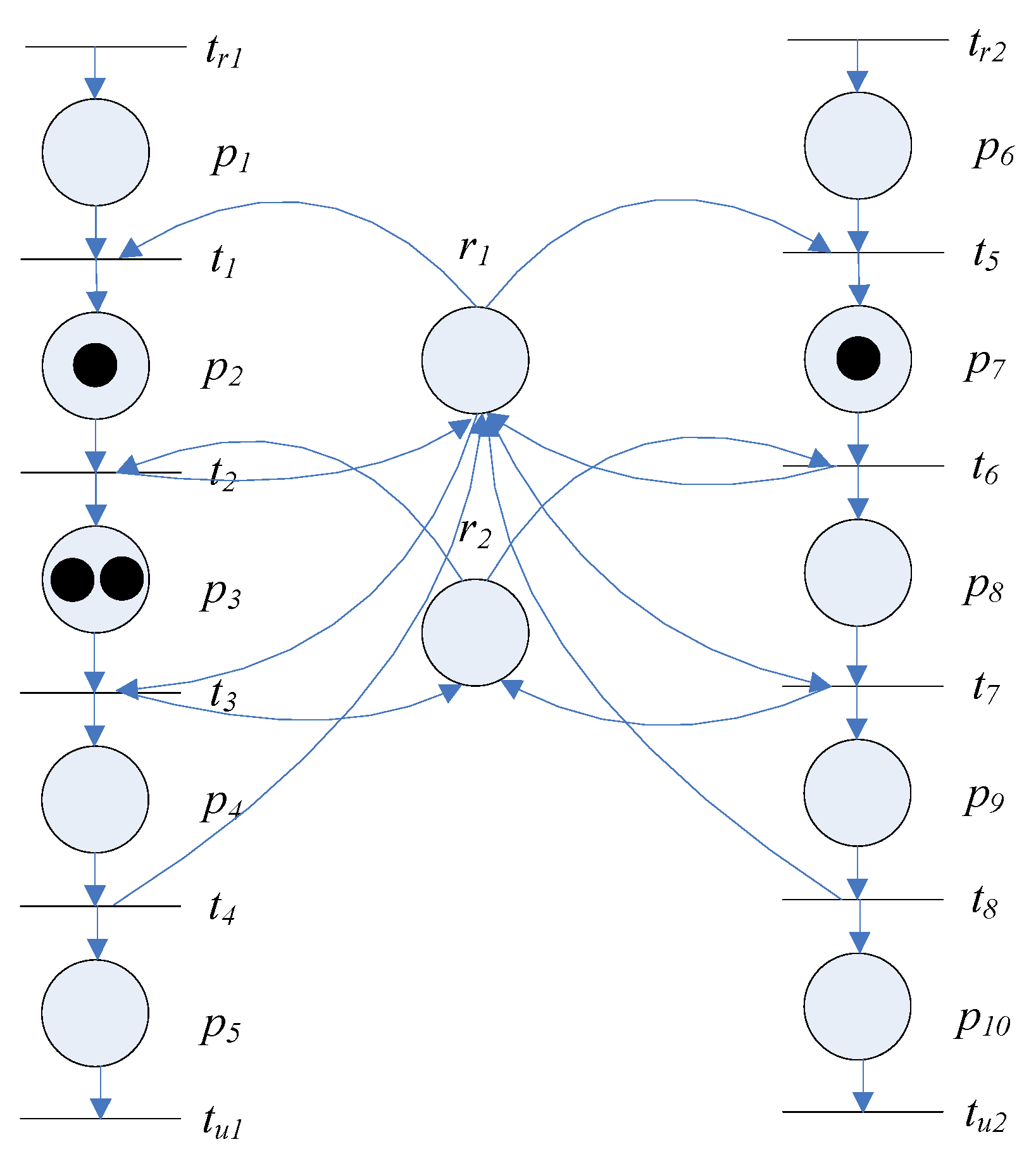
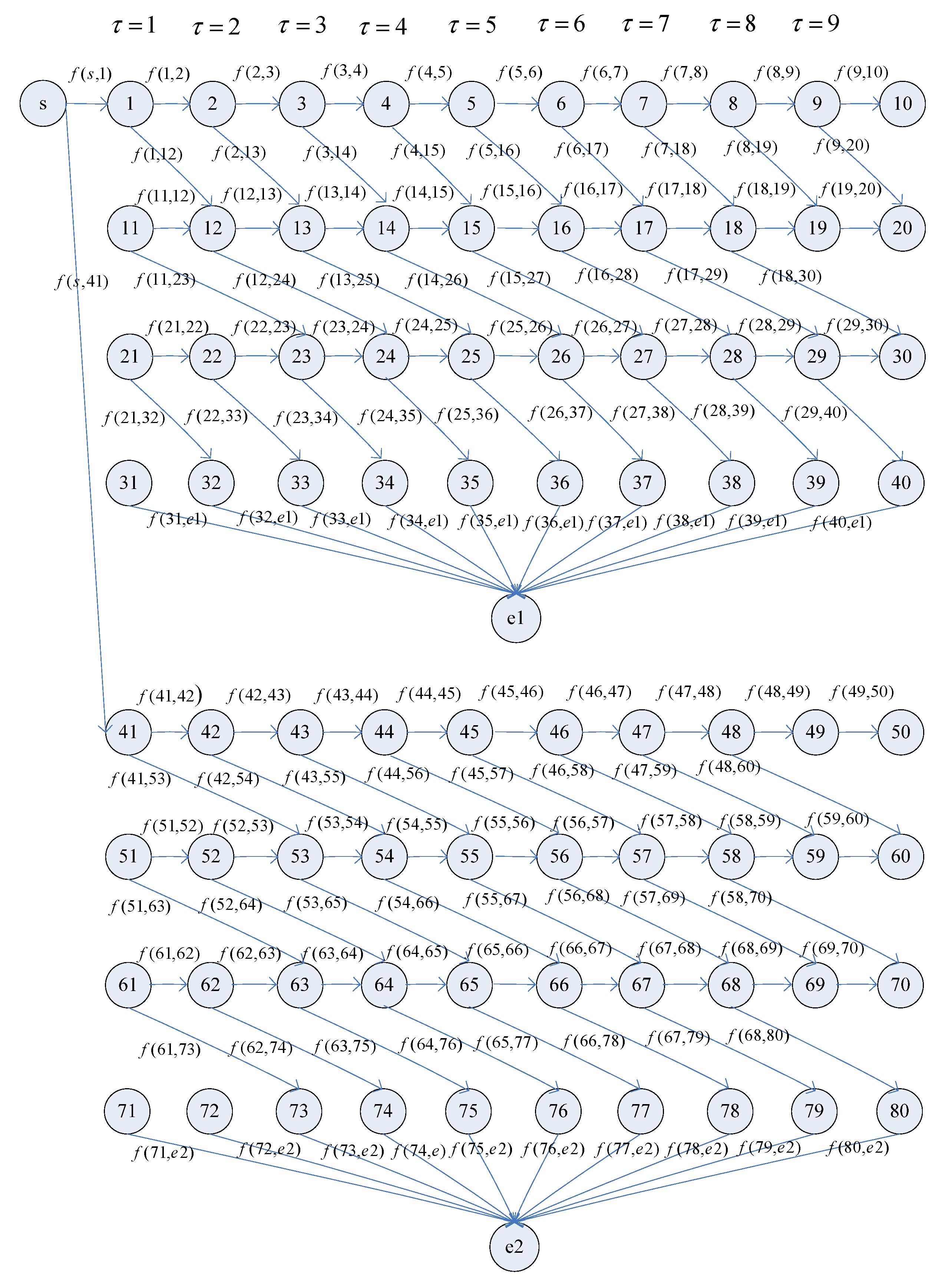
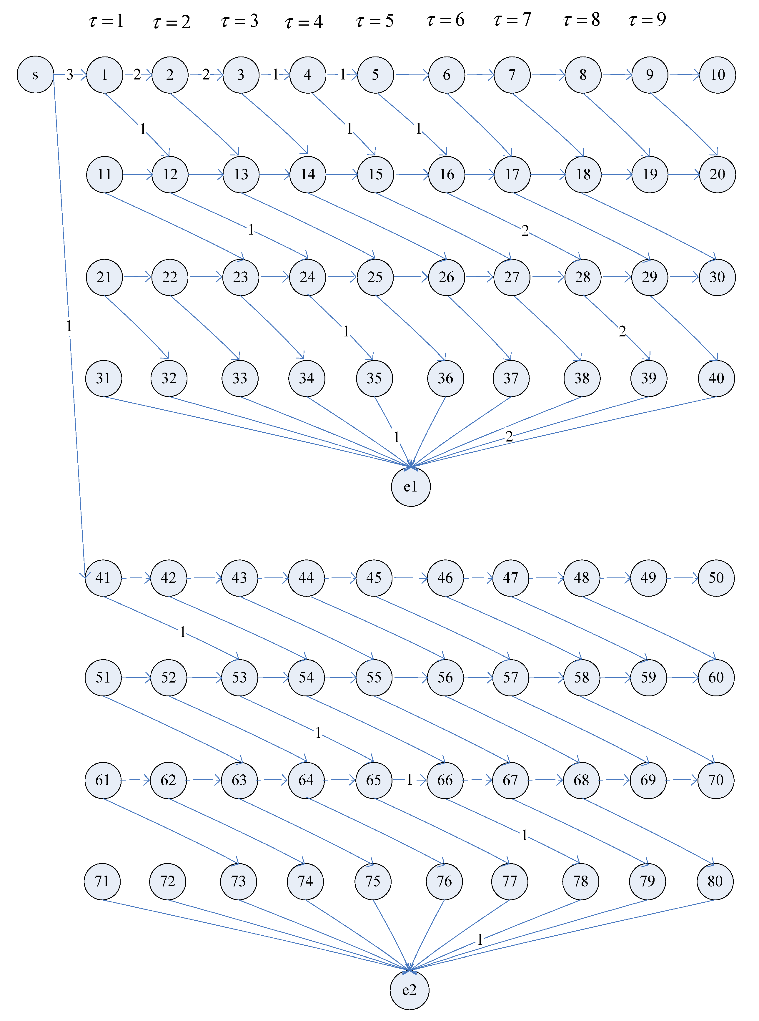

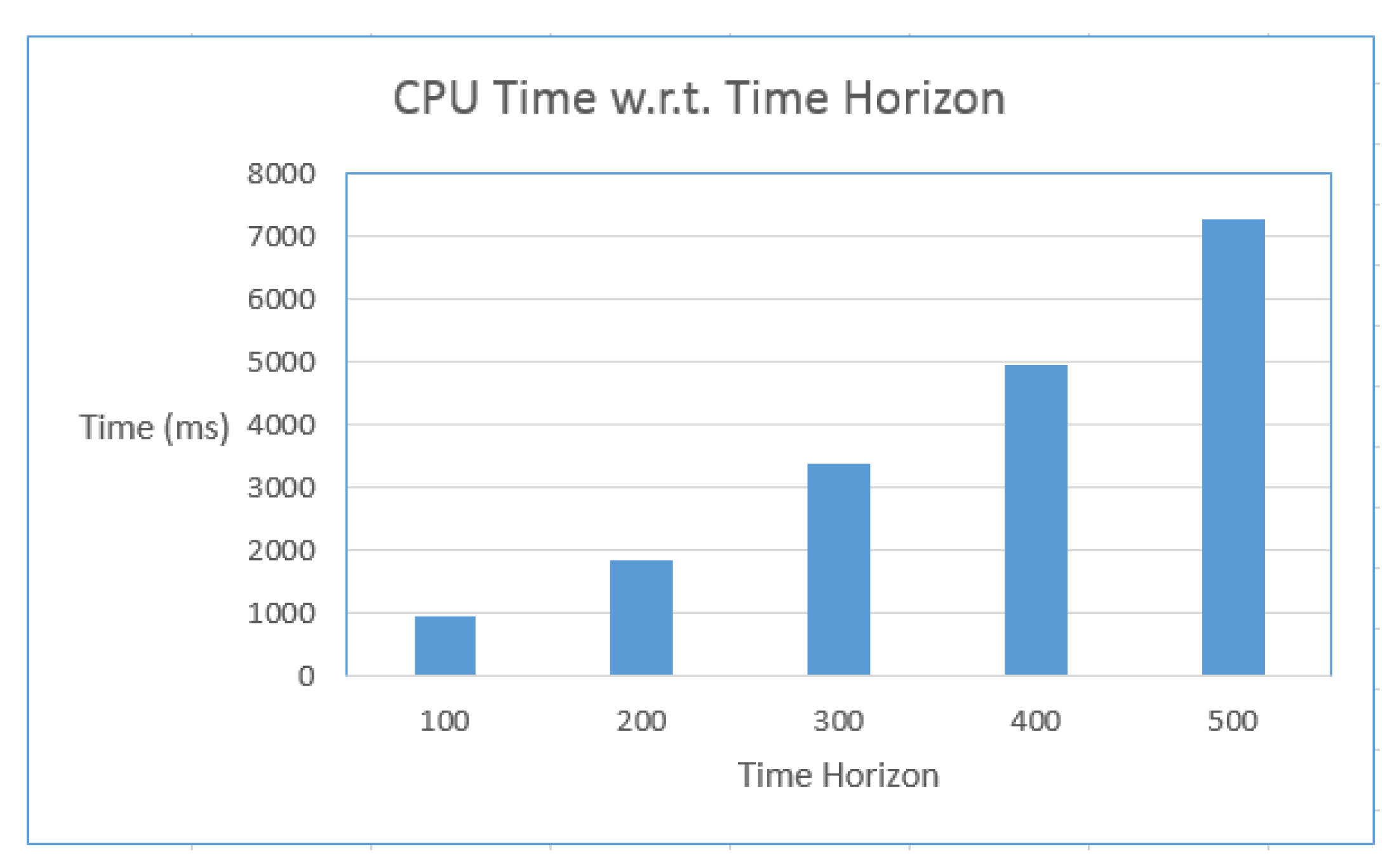

Publisher’s Note: MDPI stays neutral with regard to jurisdictional claims in published maps and institutional affiliations. |
© 2022 by the author. Licensee MDPI, Basel, Switzerland. This article is an open access article distributed under the terms and conditions of the Creative Commons Attribution (CC BY) license (https://creativecommons.org/licenses/by/4.0/).