
A Hybrid Bald Eagle Search Algorithm for Time Difference of Arrival Localization


Abstract
:1. Introduction
- Aiming at the shortcomings of TDOA localization algorithm in WSNs, which is susceptible to interference from non-visual range errors and poor localization results, a hybrid bald eagle search algorithm (HBES) is proposed to replace the mathematical analysis method to estimate the unknown node coordinates. It avoids the inverse and the derivative of the matrix in the mathematical analysis method, which can lead to unsolvable solutions.
- To enhance the optimization capability of the bald eagle search algorithm (BES), we propose to use chaotic mapping, Lévy’s flight and backward learning strategies to improve the population quality, and hybrid sine and cosine algorithms to improve the performance of the bald eagle algorithm.
- A localization model combining the TDOA algorithm and HBES algorithm is developed, and experiments are conducted to analyze the performance of the algorithm and the localization effect.
2. Background and Related Work
3. Proposed Localization Algorithm
3.1. TDOA Localization Algorithm
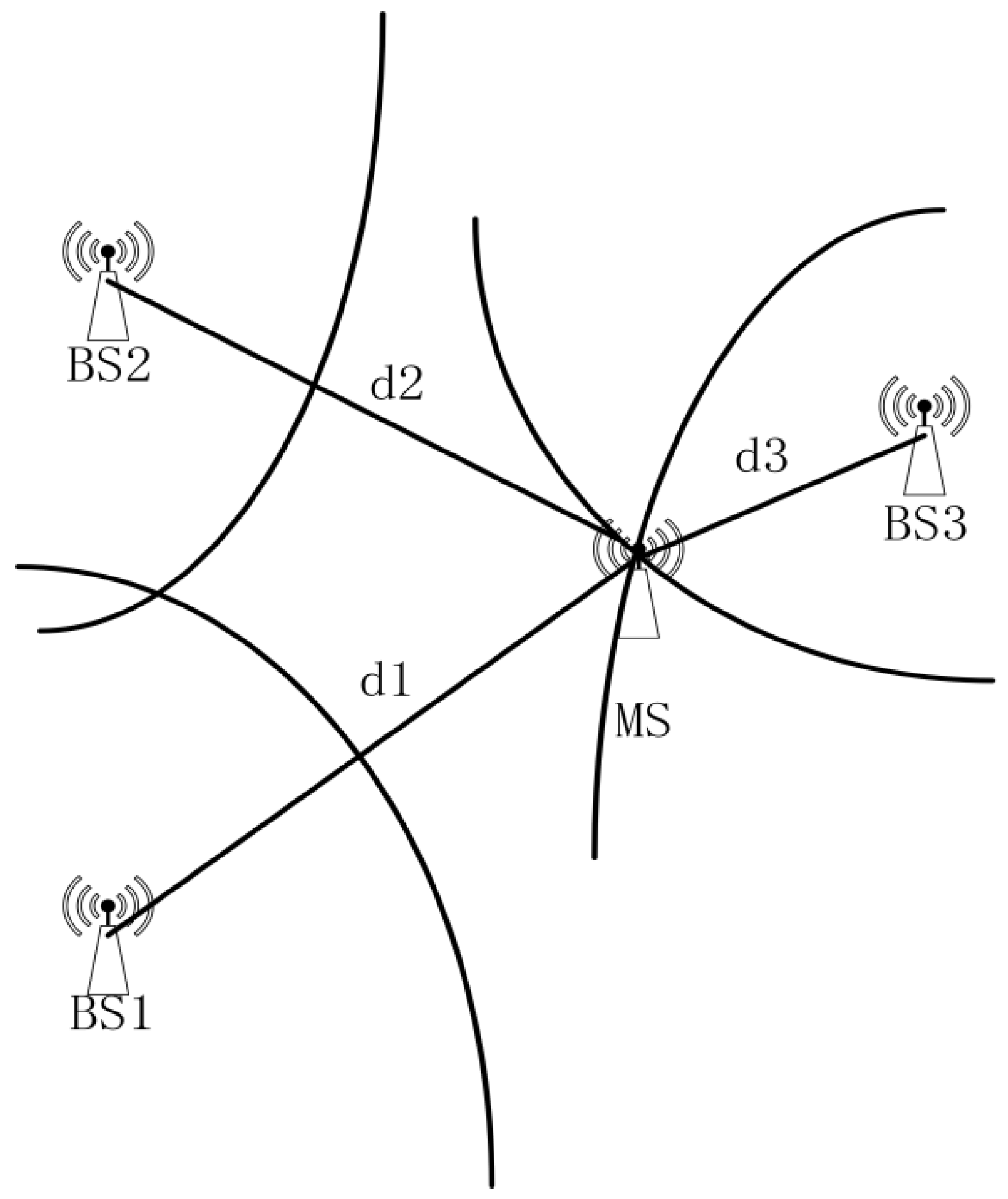
3.1.1. TDOA Positioning Principle
3.1.2. Location Model Based on Swarm Intelligence Algorithm
3.2. Hybrid Bald Eagle Search Optimization Algorithm
3.2.1. Bald Eagle Search Optimization Algorithm
3.2.2. Lévy Flight Strategy
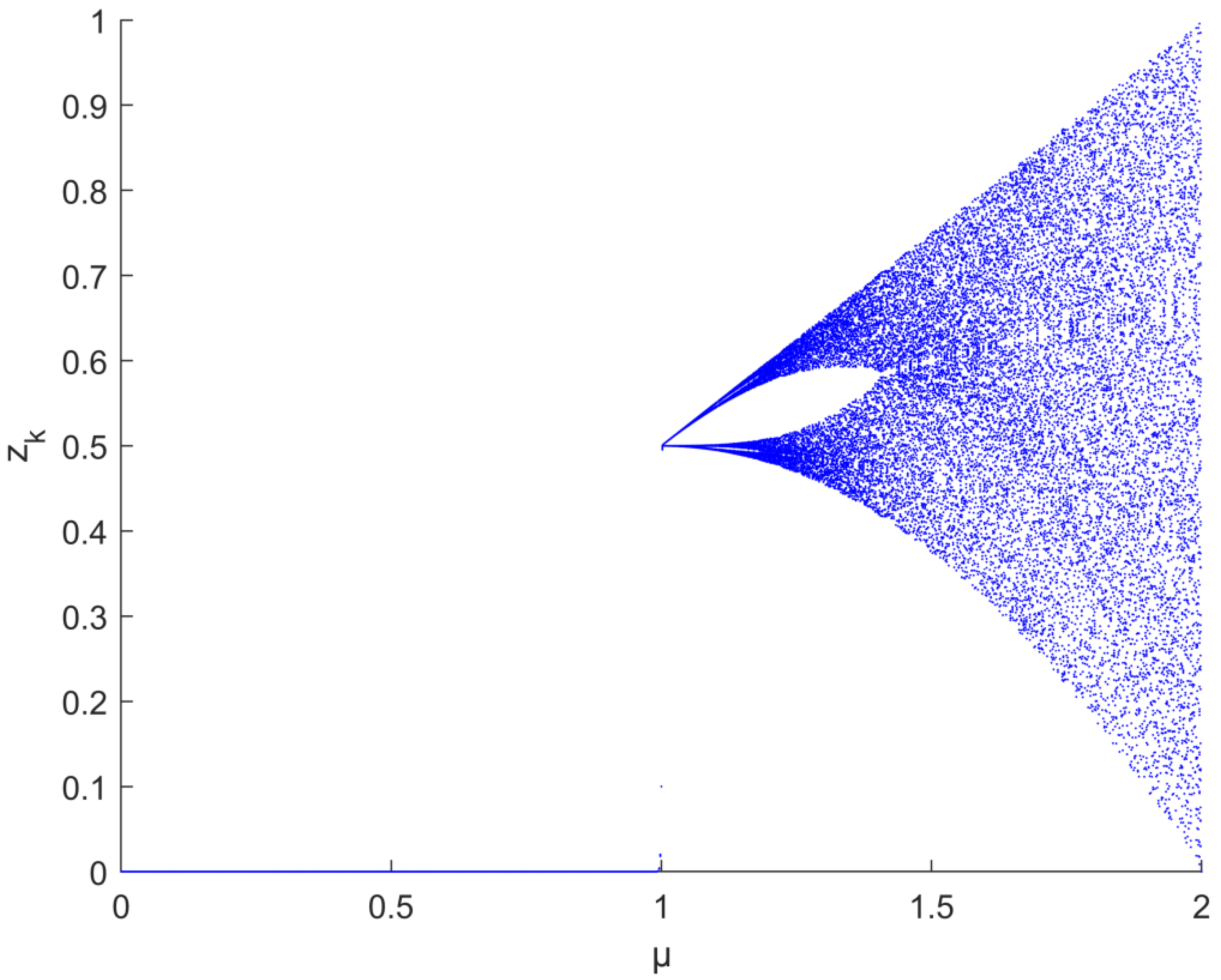
3.2.3. Chaos Mapping
3.2.4. Sine Cosine Algorithm
3.2.5. Opposition-Based Learning
3.2.6. Time Complexity Analysis
3.3. TDOA Localization Implementation Process and Pseudo Code Based on HBES
| Algorithm 1: Pseudo code of HBES-based TDOA positioning process |
|
4. Experimental Design and Analysis
4.1. Experimental Design
4.2. Performance Evaluation
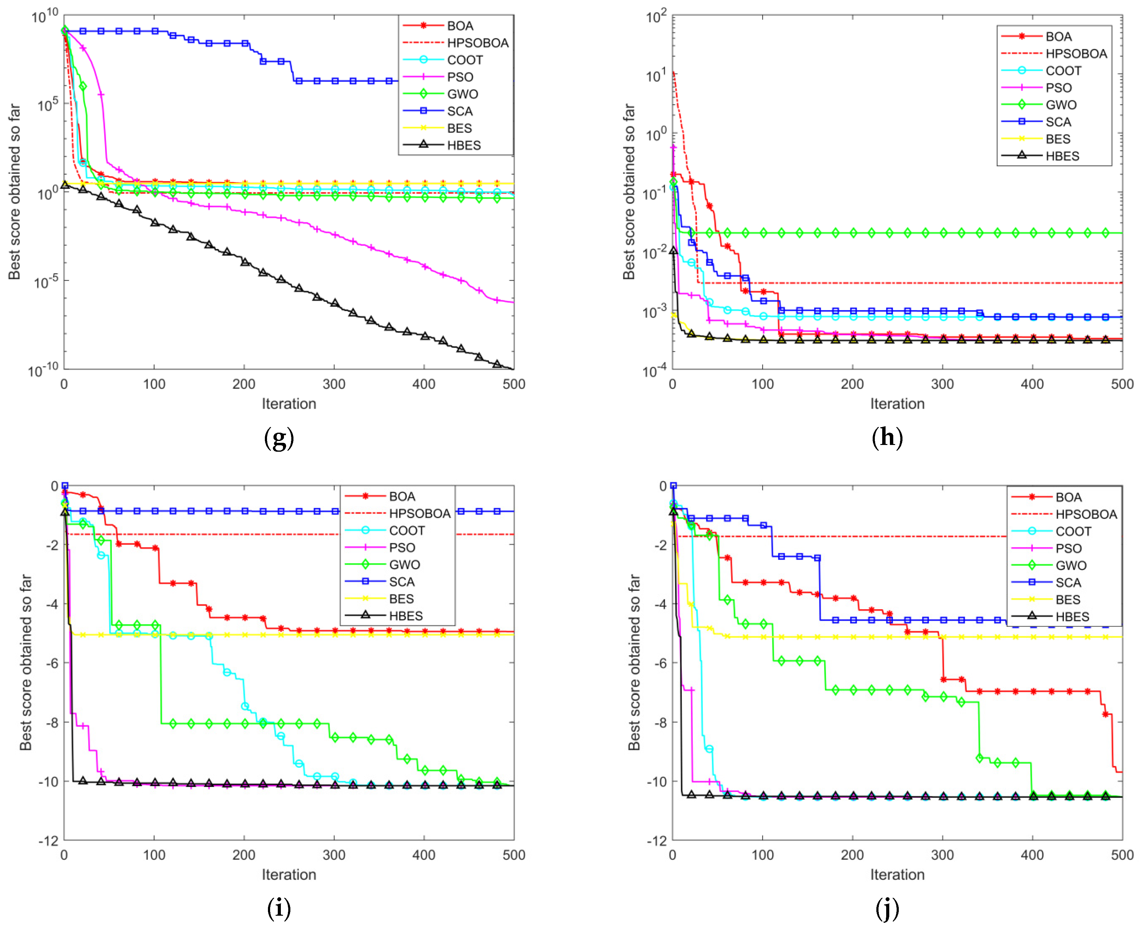
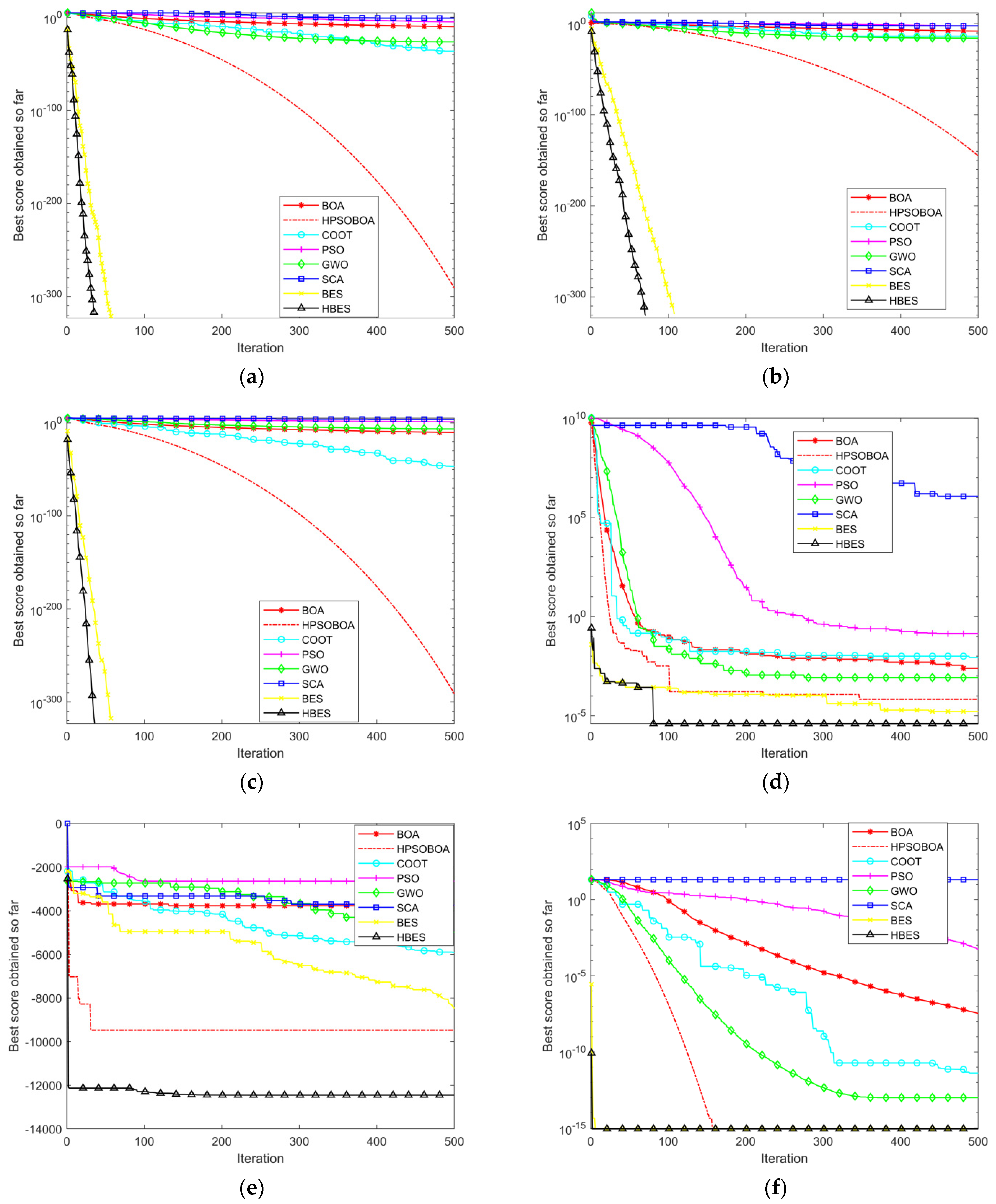
4.2.1. Comparison of Benchmark Test Function Optimization
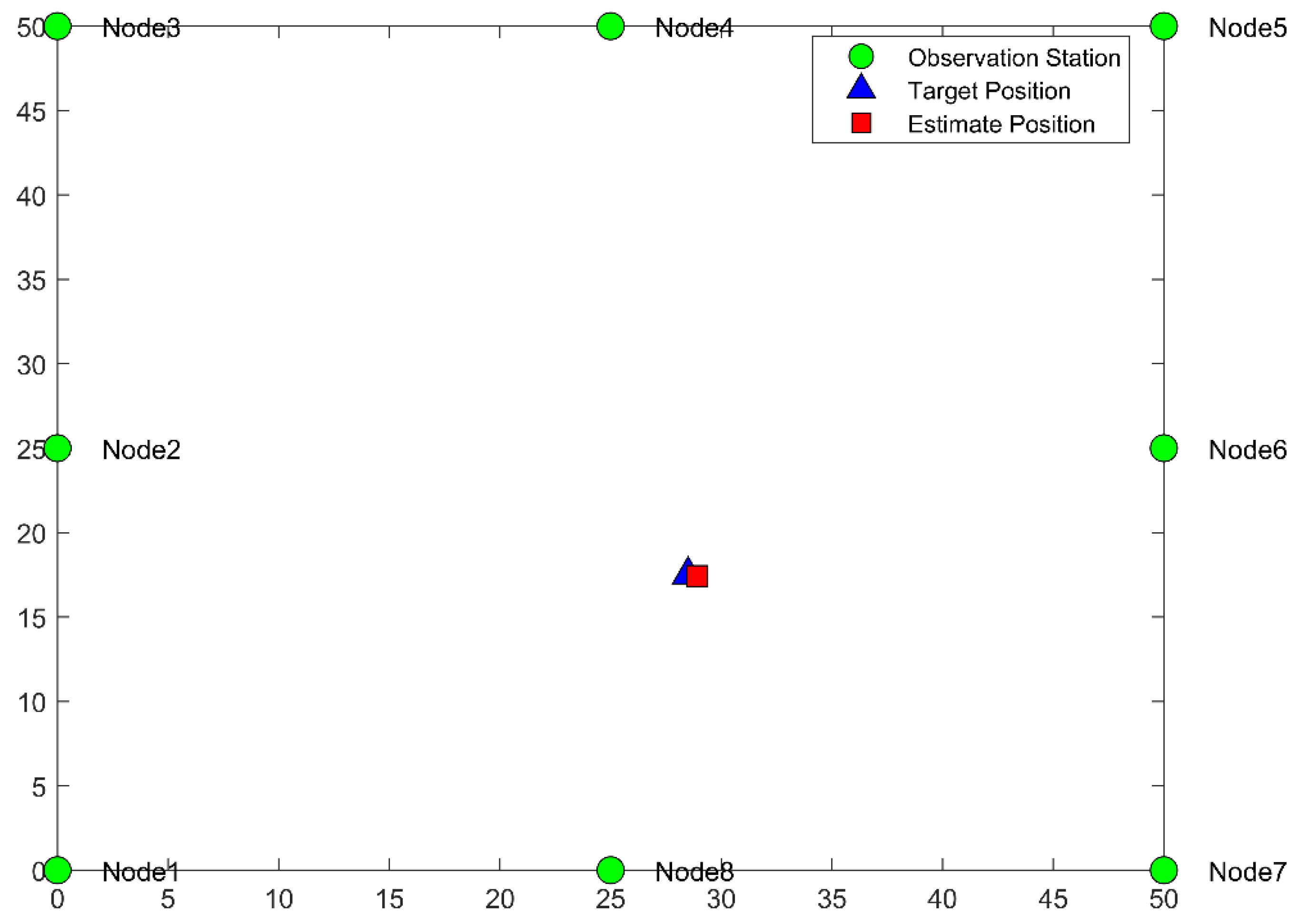
4.2.2. HBES-Based Simulation of TDOA Localization
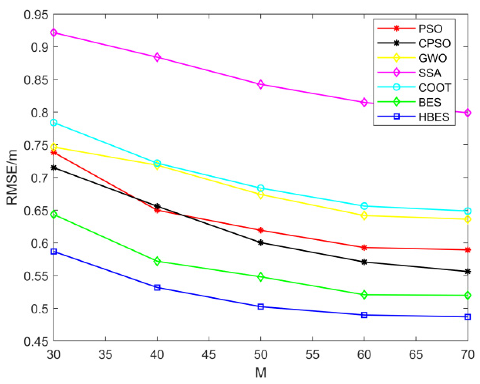
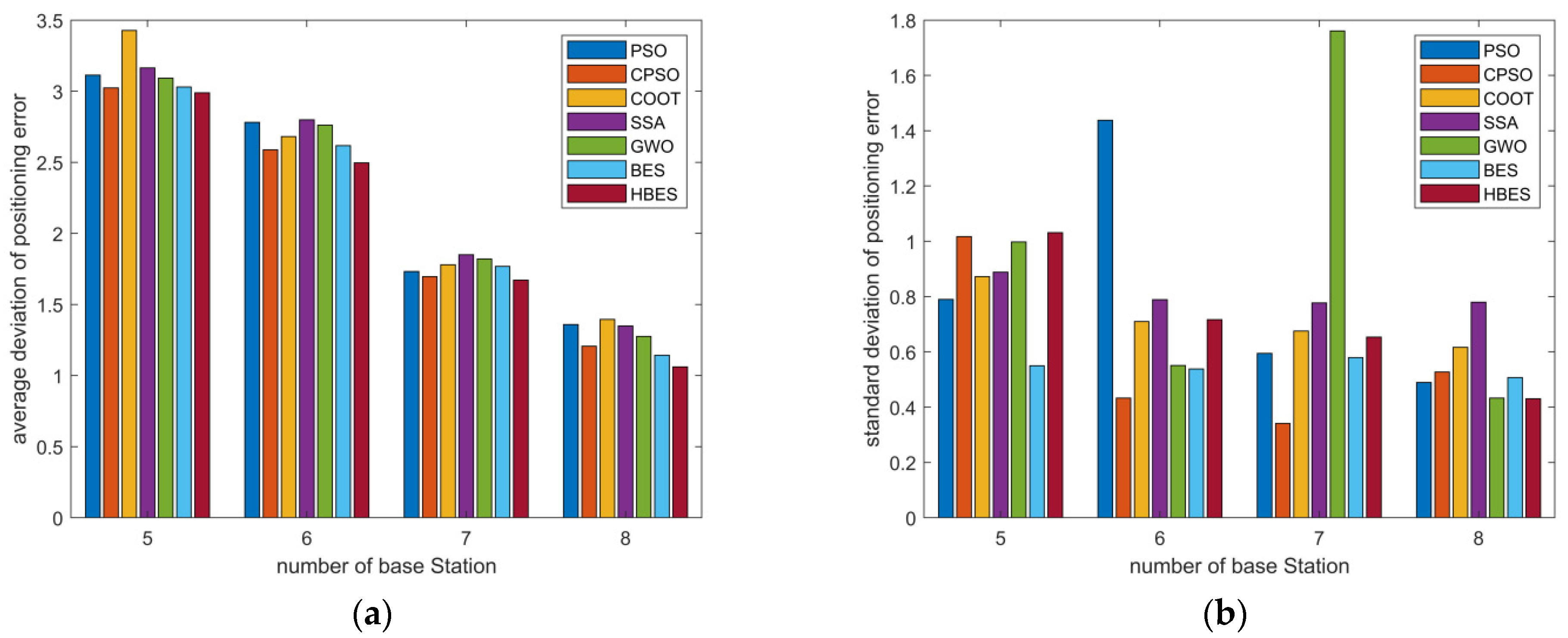
4.2.3. Analysis of the Accuracy of TDOA Positioning Based on HBES
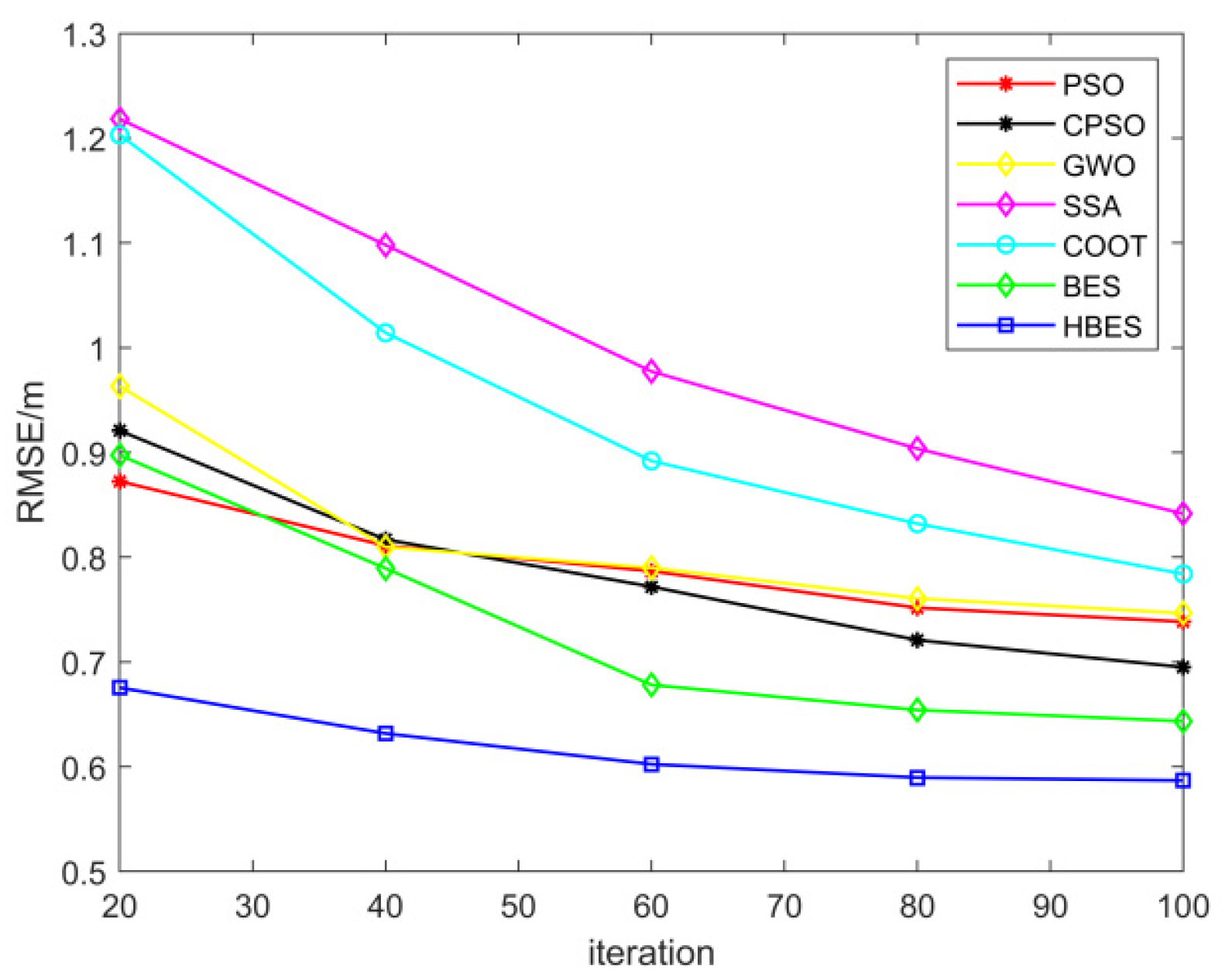
4.2.4. Analysis of the Convergence Performance of TDOA Based on HBES
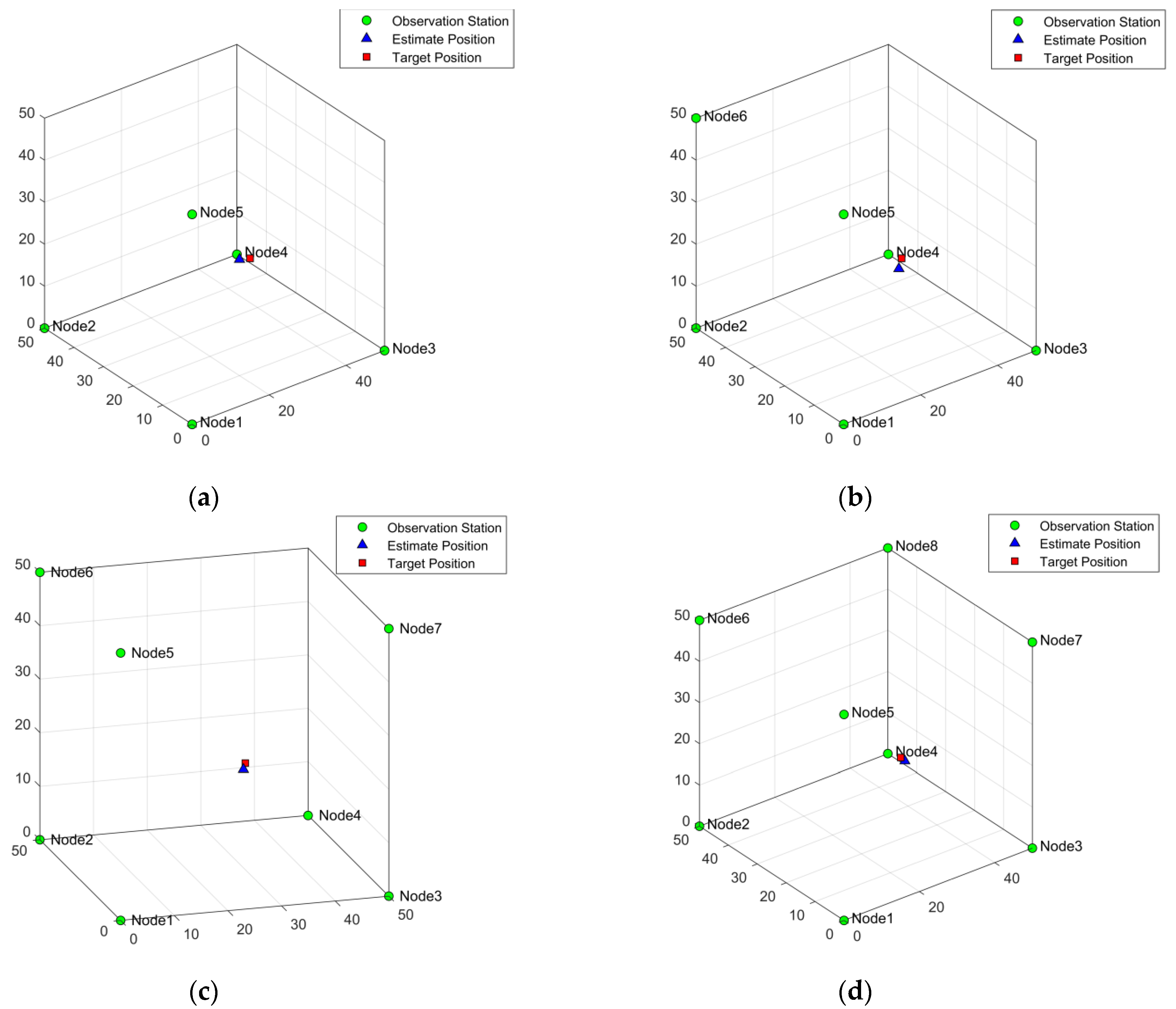
4.2.5. Comparison of 3D Scene Positioning
5. Conclusions
Author Contributions
Funding
Institutional Review Board Statement
Informed Consent Statement
Data Availability Statement
Conflicts of Interest
References
- Yaqoob, I.; Hashem, I.A.T.; Ahmed, A.; Kazmi, S.A.; Hong, C.S. Internet of things forensics: Recent advances, taxonomy, requirements, and open challenges. Futur. Gener. Comput. Syst. 2018, 92, 265–275. [Google Scholar] [CrossRef]
- Srinivasan, C.R.; Rajesh, B.; Saikalyan, P. A review on the different types of Internet of Things (IoT). J. Adv. Res. Dyn. Control Syst. 2019, 11, 154–158. [Google Scholar]
- Jagannath, J.; Polosky, N.; Jagannath, A. Machine learning for wireless communications in the Internet of Things: A comprehensive survey. Ad Hoc Netw. 2019, 93, 101913. [Google Scholar] [CrossRef] [Green Version]
- Malik, H.; Alam, M.M.; Pervaiz, H. Radio resource management in NB-IoT systems: Empowered by interference prediction and flexible duplexing. IEEE Netw. 2019, 34, 144–151. [Google Scholar] [CrossRef]
- KKhan, S.Z.; Malik, H.; Sarmiento, J.L.R.; Alam, M.M.; Le Moullec, Y. DORM: Narrowband IoT Development Platform and Indoor Deployment Coverage Analysis. Procedia Comput. Sci. 2019, 151, 1084–1091. [Google Scholar] [CrossRef]
- Rashid, B.; Rehmani, M.H. Applications of wireless sensor networks for urban areas: A survey. J. Netw. Comput. Appl. 2016, 60, 192–219. [Google Scholar] [CrossRef]
- Navarro, M.; Davis, T.W.; Liang, Y. ASWP: A long-term WSN deployment for environmental monitoring. In Proceedings of the 12th International Conference on Information Processing in Sensor Networks, Philadelphia, PA, USA, 8–13 April 2013; pp. 351–352. [Google Scholar]
- Chiang, S.Y.; Kan, Y.C.; Tu, Y.C. A preliminary activity recognition of WSN data on ubiquitous health care for physical therapy. In Recent Progress in Data Engineering and Internet Technology; Springer: Berlin/Heidelberg, Germany, 2013; pp. 461–467. [Google Scholar]
- Shi, L.; Wang, F.B. Range-free localization mechanism and algorithm in wireless sensor networks. Comput. Eng. Appl. 2004, 40, 127–130. [Google Scholar]
- Liu, F.; Li, X.; Wang, J.; Zhang, J. An Adaptive UWB/MEMS-IMU Complementary Kalman Filter for Indoor Location in NLOS Environment. Remote Sens. 2019, 11, 2628. [Google Scholar] [CrossRef] [Green Version]
- Xiong, H.; Chen, Z.; An, W.; Yang, B. Robust TDOA Localization Algorithm for Asynchronous Wireless Sensor Networks. Int. J. Distrib. Sens. Netw. 2015, 11, 598747. [Google Scholar] [CrossRef]
- Meyer, F.; Tesei, A.; Win, M.Z. Localization of multiple sources using time-difference of arrival measurements. In Proceedings of the 2017 IEEE International Conference on Acoustics, Speech and Signal Processing (ICASSP), New Orleans, LA, USA, 5–9 March 2017; pp. 3151–3155. [Google Scholar]
- Tomic, S.; Beko, M.; Camarinha-Matos, L.M.; Oliveira, L.B. Distributed Localization with Complemented RSS and AOA Measurements: Theory and Methods. Appl. Sci. 2019, 10, 272. [Google Scholar] [CrossRef] [Green Version]
- Mass-Sanchez, J.; Ruiz-Ibarra, E.; Gonzalez-Sanchez, A.; Espinoza-Ruiz, A.; Cortez-Gonzalez, J. Factorial Design Analysis for Localization Algorithms. Appl. Sci. 2018, 8, 2654. [Google Scholar] [CrossRef] [Green Version]
- Beni, G.; Wang, U. Swarm intelligence in cellular robotic systems. In Robots and Biological Systems: Towards a New Bionics? Springer: Berlin/Heidelberg, Germany, 1993. [Google Scholar]
- Colorni, A.; Dorigo, M.; Maniezzo, V. Distributed optimization by ant colonies. In Proceedings of the 1st European Conference on Artificial Life, Paris, France, 11–13 December 1991; pp. 134–142. [Google Scholar]
- Colorni, A.; Dorigo, M.; Maniezzo, V. An investigation of some properties of an ant algorithm. In Proceedings of the Parallel Problem Solving from Nature Conference, Brussels, Belgium, 28–30 September 1992; pp. 509–520. [Google Scholar]
- Colorni, A.; Dorigo, M.; Maniezzo, V. Ant system for job shop scheduling. Oper. Res. Stat. Comput. Sci. 1994, 34, 39–53. [Google Scholar]
- Smets, P.; Kennes, R. The transferable belief model. Artif. Intell. 1994, 66, 191–234. [Google Scholar] [CrossRef]
- Vaghefi, R.M.; Buehrer, R.M. Cooperative Joint Synchronization and Localization in Wireless Sensor Networks. IEEE Trans. Signal Process. 2015, 63, 3615–3627. [Google Scholar] [CrossRef]
- Le, T.-K.; Ono, N. Closed-Form and Near Closed-Form Solutions for TDOA-Based Joint Source and Sensor Localization. IEEE Trans. Signal Process. 2016, 65, 1207–1221. [Google Scholar] [CrossRef]
- Foy, W.H. Position-location solutions by Taylor-series estimation. IEEE Trans. Aerosp. Electron. Syst. 2007, AES-12, 187–194. [Google Scholar] [CrossRef]
- Xiaomei, Q.; Lihua, X. An efficient convex constrained weighted least squares source localization algorithm based on TDOA measurements. Signal Process. 2016, 119, 142–152. [Google Scholar]
- Jihao, Y.; Qun, W.; Shiwen, Y. A simple and accurate TDOA-AOA localization method using two stations. IEEE Signal Process. Lett. 2015, 23, 144–148. [Google Scholar]
- Kenneth, W.K.; Jun, Z. Particle swarm optimization for time-difference-of-arrival based localization. In Proceedings of the Signal Processing Conference, Poznan, Poland, 3–7 September 2007; pp. 414–417. [Google Scholar]
- Tao, C.; Mengxin, W.; Xiangsong, H. Passive time difference location based on salp swarm algorithm. J. Electron. Inf. Technol. 2018, 40, 1591–1597. [Google Scholar]
- Yue, Y.; Cao, L.; Hu, J. A novel hybrid location algorithm based on chaotic particle swarm optimization for mobile position estimatio. IEEE Access 2019, 7, 58541–58552. [Google Scholar] [CrossRef]
- Shengliang, W.; Genyou, L.; Ming, G. Application of improved adaptive genetic algorithm in TDOA localization. Syst. Eng. Electron. 2019, 41, 254–258. [Google Scholar]
- Wolpert, D.H.; Macready, W.G. No free lunch theorems for optimization. IEEE Trans. Evol. Comput. 1997, 1, 67–82. [Google Scholar] [CrossRef] [Green Version]
- Alsattar, H.A.; Zaidan, A.A.; Zaidan, B.B. Novel meta-heuristic bald eagle search optimization algorithm. Artif. Intell. Rev. 2020, 53, 2237–2264. [Google Scholar] [CrossRef]
- Yanhong, F.; Jianqin, L.; Yizhao, H. Dynamic population firefly algorithm based on chaos theory. Comput. Appl. 2013, 33, 796–799. [Google Scholar]
- Leccardi, M. Comparison of three algorithms for Levy noise generation. In Proceedings of the fifth EUROMECH Nonlinear Dynamics Conference, Eindhoven, The Netherlands, 7–12 August 2005. [Google Scholar]
- Jiakui, Z.; Lijie, C.; Qing, G. Grey Wolf optimization algorithm based on Tent chaotic sequence. Microelectron. Comput. 2018, 3, 11–16. [Google Scholar]
- Chunmei, T.; Guobin, C.; Chao, L. Research on chaotic feedback adaptive whale optimization algorithm. Stat. Decis. Mak. 2019, 35, 17–20. [Google Scholar]
- Mirjalili, S. SCA: A sine cosine algorithm for solving optimization problems. Knowl.-Based Syst. 2016, 96, 120–133. [Google Scholar] [CrossRef]
- Tizhoosh, H.R. Opposition-based learning: A new scheme for machine intelligence. In Proceedings of the International Conference on Computational Intelligence for Modelling, Control and Automation and International Conference on Intelligent Agents, Web Technologies and Internet Commerce (CIMCA-IAWTIC’06), Vienna, Austria, 28–30 November 2005; pp. 695–701. [Google Scholar]
- Shi, Y.; Eberhart, R. A Modified Particle Swarm Optimizer. In Proceedings of the 1998 IEEE International Conference on Evolutionary Computation Proceedings, Anchorage, UK, 4–9 May 1998; pp. 69–73. [Google Scholar]
- Mirjalili, S.; Mirjalili, S.M. Lewis A. Grey wolf optimizer. Adv. Eng. Softw. 2014, 69, 46–61. [Google Scholar] [CrossRef] [Green Version]
- Naruei, I.; Keynia, F. A new optimization method based on COOT bird natural life model. Expert Syst. Appl. 2021, 183, 115352. [Google Scholar] [CrossRef]
- Arora, S.; Singh, S. Butterfly optimization algorithm: A novel approach for global optimization. Soft Comput. 2019, 23, 715–734. [Google Scholar] [CrossRef]
- Mengjian, Z.; Daoyin, L.; Tao, Q.; Jing, Y. A Chaotic Hybrid Butterfly Optimization Algorithm with Particle Swarm Optimization for High-Dimensional Optimization Problems. Symmetry 2020, 12, 1800. [Google Scholar]


| Function Classification | Test Functions | Dimension | Range of Values | Optimum Value |
|---|---|---|---|---|
| single-peaked functions | 30 | [−100, 100] | 0 | |
| 30 | [−10, 10] | 0 | ||
| 30 | [−100, 100] | 0 | ||
| 30 | [−100, 100] | 0 | ||
| 30 | [−30, 30] | 0 | ||
| 30 | [−100, 100] | 0 | ||
| 30 | [−128, 128] | 0 | ||
| multi-peaked functions | 30 | [−500, 500] | −418 × n | |
| 30 | [−5.12, 5.12] | 0 | ||
| 30 | [−32, 32] | 0 | ||
| 30 | [−600, 600] | 0 | ||
| 30 | [−50, 50] | 0 | ||
| 30 | [−50, 50] | 0 | ||
| 2 | [−65, 65] | 1 | ||
| fixed-dimensional functions | 4 | [−5, 5] | 0.0003 | |
| 2 | [−5, 5] | −1.0316 | ||
| 2 | [−5, 5] | 0.398 | ||
| 2 | [−2, 2] | 3 | ||
| 2 | [1, 3] | −3.86 | ||
| 6 | [0, 1] | −3.32 | ||
| 4 | [0, 10] | −10.1532 | ||
| 4 | [0, 10] | −10.4028 | ||
| 4 | [0, 10] | −10.5363 |
| Test Function | Indicators | PSO | BOA | HPSOBOA | SCA | GWO | COOT | BES | HBES |
|---|---|---|---|---|---|---|---|---|---|
| mean | 1.15 × 10⁻⁵ | 7.71 × 10⁻¹¹ | 1.862 × 10−290 | 23.2423 | 1.25 × 10⁻²⁷ | 2.07 × 10⁻¹³ | 0 | 0 | |
| std | 2.57 × 10⁻⁵ | 6.71 × 10⁻¹² | 0 | 68.9556 | 2.1 × 10⁻²⁷ | 1.47 × 10⁻¹² | 0 | 0 | |
| SR(%) | 0 | 0 | 100 | 0 | 0 | 76 | 100 | 100 | |
| mean | 0.0063 | 2.33 × 10⁻⁸ | 8.62 × 10−146 | 0.0306 | 1.07 × 10⁻¹⁶ | 4.05 × 10⁻⁸ | 0 | 0 | |
| std | 0.0124 | 6.46 × 10⁻⁹ | 5.59 × 10−146 | 0.0439 | 8.79 × 10⁻¹⁷ | 2.86 × 10⁻⁷ | 0 | 0 | |
| SR(%) | 0 | 0 | 100 | 0 | 0 | 0 | 100 | 100 | |
| mean | 0.4956 | 6.2 × 10⁻¹¹ | 1.096 × 10−289 | 92.85 | 7.28 × 10⁻⁷ | 2.02 × 10⁻¹⁰ | 0 | 0 | |
| std | 0.2497 | 7.91 × 10⁻¹² | 0 | 53.39 | 8.65 × 10⁻⁷ | 1.39 × 10⁻⁹ | 0 | 0 | |
| SR(%) | 0 | 0 | 100 | 0 | 0 | 0 | 100 | 100 | |
| mean | 0.5364 | 3.38 × 10⁻⁸ | 2.52 × 10−146 | 34.6610 | 8.15 × 10⁻⁷ | 4.04 × 10⁻¹³ | 0 | 0 | |
| std | 0.4226 | 3.38 × 10⁻⁹ | 1.2 × 10−147 | 11.1013 | 9.05 × 10⁻⁷ | 2.66 × 10⁻¹⁶ | 0 | 0 | |
| SR(%) | 0 | 0 | 100 | 0 | 0 | 0 | 100 | 100 | |
| mean | 42.62 | 28.9069 | 28.776 | 953.3394 | 27.2613 | 44.97 | 19.0639 | 20.4183 | |
| std | 26.64 | 0.0263 | 0.0644 | 3.37 × 10³ | 0.7647 | 44.44 | 1.4906 | 0.2718 | |
| SR(%) | 0 | 0 | 0 | 0 | 0 | 0 | 0 | 0 | |
| mean | 1.15 × 10⁻⁶ | 5.4064 | 0.0416 | 40.6717 | 0.6766 | 0.2605 | 1.34 × 10⁻¹⁸ | 2.13 × 10⁻¹⁸ | |
| std | 2.04 × 10⁻⁵ | 0.5654 | 0.0318 | 166.8152 | 0.3671 | 0.2008 | 4.29 × 10⁻¹⁸ | 5.05 × 10⁻¹⁸ | |
| SR(%) | 0 | 0 | 0 | 0 | 0 | 0 | 0 | 0 | |
| mean | 0.0832 | 0.0019 | 2.14 × 10⁻⁵ | 112.9 | 0.0022 | 0.0055 | 3.98 × 10⁻⁵ | 2.47 × 10⁻⁴ | |
| std | 0.0377 | 6.81 × 10⁻⁴ | 1.05 × 10⁻⁴ | 248.6 | 0.0013 | 0.0045 | 3.77 × 10⁻⁵ | 0.0012 | |
| SR(%) | 0 | 0 | 0 | 0 | 0 | 0 | 0 | 0 | |
| mean | −2.79 × 10³ | −4.04 × 10³ | −9.745 × 10³ | −3.73 × 10³ | −5.97 × 10³ | −7.44 × 10³ | −7.48 × 10³ | −1.24 × 10⁴ | |
| std | 406.595 | 343.2 | 1.367 × 10³ | 308.97 | 840.6115 | 1.05 × 10³ | 1.60 × 10³ | 1.09 × 10³ | |
| SR(%) | 0 | 0 | 0 | 0 | 0 | 0 | 0 | 78 | |
| mean | 45.8288 | 32.8474 | 0.0643 | 38.6612 | 2.5001 | 1.04 × 10⁻¹² | 0 | 0 | |
| std | 14.4283 | 69.8399 | 0.1818 | 34.3327 | 3.299 | 6.67 × 10⁻¹² | 0 | 0 | |
| SR(%) | 0 | 0 | 0 | 0 | 0 | 84 | 100 | 100 | |
| mean | 0.0012 | 2.78 × 10⁻⁸ | 8.88 × 10⁻¹⁶ | 14.1827 | 1.05 × 10⁻¹³ | 8.39 × 10⁻¹³ | 8.88 × 10⁻¹⁶ | 8.88 × 10⁻¹⁶ | |
| std | 5.68 × 10⁻⁴ | 5.61 × 10⁻⁹ | 0 | 8.9091 | 1.85 × 10⁻¹⁴ | 5.1 × 10⁻¹² | 0 | 0 | |
| SR(%) | 0 | 0 | 0 | 0 | 0 | 0 | 0 | 0 | |
| mean | 43.0227 | 1.18 × 10⁻¹¹ | 0 | 0.9740 | 0.0028 | 2.4 × 10⁻¹¹ | 0 | 0 | |
| std | 6.8557 | 1.06 × 10⁻¹¹ | 0 | 0.4335 | 0.0066 | 1.7 × 10⁻¹⁰ | 0 | 0 | |
| SR(%) | 0 | 0 | 100 | 0 | 0 | 72 | 100 | 100 | |
| mean | 0.7678 | 0.4866 | 0.0019 | 1.06 × 10³ | 0.0398 | 0.2583 | 5.79 × 10⁻²⁰ | 5.18 × 10⁻²⁰ | |
| std | 0.6487 | 0.1274 | 0.0014 | 5.83 × 10³ | 0.0170 | 0.6319 | 3.68 × 10⁻¹⁹ | 1.02 × 10⁻¹⁸ | |
| SR(%) | 0 | 0 | 0 | 0 | 0 | 0 | 0 | 0 | |
| mean | 0.0015 | 2.777 | 0.911 | 788.27 | 0.6138 | 0.4766 | 2.8705 | 0.0059 | |
| std | 0.0044 | 0.2658 | 0.7025 | 180.74 | 0.2386 | 0.4419 | 0.4485 | 0.0144 | |
| SR(%) | 0 | 0 | 0 | 0 | 0 | 0 | 0 | 0 | |
| mean | 1.5131 | 1.1505 | 3.1745 | 1.9508 | 4.2161 | 0.9980 | 5.3268 | 2.5651 | |
| std | 1.1153 | 0.3856 | 2.7582 | 1.0009 | 3.7155 | 2.3 × 10⁻¹³ | 5.2344 | 3.2754 | |
| SR(%) | 0 | 0 | 0 | 0 | 0 | 0 | 0 | 0 | |
| mean | 5.85 × 10⁻⁴ | 3.72 × 10⁻⁴ | 0.0015 | 0.0011 | 0.0044 | 7.02 × 10⁻⁴ | 3.68 × 10⁻⁴ | 3.07 × 10⁻⁴ | |
| std | 4.37 × 10⁻⁴ | 5.26 × 10⁻⁵ | 7.9276 × 10⁻⁴ | 3.807 × 10⁻⁴ | 0.008 | 2.59 × 10⁻⁴ | 2.22 × 10⁻⁴ | 3.42 × 10⁻⁸ | |
| SR(%) | 0 | 0 | 0 | 0 | 0 | 0 | 0 | 0 | |
| mean | −1.0316 | −1.0316 | −0.6435 | −1.0316 | −1.0316 | −1.0316 | −1.0316 | −1.0316 | |
| std | 2.61 × 10⁻¹⁶ | 5.6 × 10⁻⁵ | 0.0972 | 6.1034 × 10⁻⁵ | 2.14 × 10⁻⁸ | 3.31 × 10⁻¹² | 1.48 × 10⁻⁷ | 1.53 × 10⁻⁹ | |
| SR(%) | 100 | 64 | 0 | 78 | 100 | 100 | 100 | 100 | |
| mean | 0.3979 | 0.4514 | 0.3979 | 0.4010 | 0.3979 | 0.3979 | 0.3979 | 0.3979 | |
| std | 0 | 0.0078 | 4.39 × 10⁻⁶ | 0.0032 | 3.79 × 10⁻⁶ | 0.0012 | 4.71 × 10⁻⁷ | 2.28 × 10⁻⁸ | |
| SR(%) | 0 | 0 | 0 | 0 | 0 | 0 | 0 | 0 | |
| mean | 3 | 3.5621 | 28.0966 | 3.0002 | 3 | 3 | 3 | 3 | |
| std | 1.37 × 10⁻¹⁵ | 3..6640 | 5.8650 | 3.02 × 10⁻⁴ | 3.74 × 10⁻⁵ | 1.83 × 10⁻¹² | 6.085 × 10⁻¹⁶ | 7.4587 × 10⁻¹⁸ | |
| SR(%) | 100 | 0 | 0 | 0 | 92 | 100 | 100 | 100 | |
| mean | −3.8628 | −3.8568 | −3.1973 | −3.8543 | −3.8615 | −3.8628 | −3.8628 | −3.8628 | |
| std | 1.3 × 10⁻¹⁵ | 0.0089 | 0.0094 | 0.0027 | 0.0023 | 1.89 × 10⁻¹¹ | 1.34 × 10⁻¹⁵ | 2.34 × 10⁻¹⁵ | |
| SR(%) | 0 | 0 | 0 | 0 | 0 | 0 | 0 | 0 | |
| mean | −3.2649 | −3.0238 | −2.0792 | −2.8994 | −3.2738 | −3.2958 | −3.2602 | −3.2673 | |
| std | 0.06 | 0.1649 | 8.97 × 10⁻¹⁶ | 0.3445 | 0.0675 | 0.0498 | 0.06 | 0.04 | |
| SR(%) | 0 | 0 | 0 | 0 | 0 | 0 | 0 | 0 | |
| mean | −5.4891 | −6.9961 | −1.6612 | −2.4205 | −9.3193 | −9.0522 | −7.505 | −10.1513 | |
| std | 3.2346 | 1.7411 | 0.0272 | 1.9668 | 1.9313 | 2.5766 | 2.5702 | 3.48 × 10⁻⁵ | |
| SR(%) | 32 | 0 | 0 | 0 | 0 | 78 | 48 | 94 | |
| mean | −7.1406 | −7.4507 | −1.6867 | −3.5481 | −10.0364 | −9.4728 | −7.5917 | −10.2694 | |
| std | 3.6318 | 1.6058 | 0.006 | 1.7069 | 1.4839 | 2.3699 | 2.7382 | 0.94 | |
| SR(%) | 0 | 0 | 0 | 0 | 0 | 0 | 0 | 0 | |
| mean | −5.9766 | −8.0935 | −1.7266 | −3.9590 | −10.2949 | −10.0932 | −8.1434 | −10.4024 | |
| std | 3.5971 | 1.383 | 0.004 | 1.6797 | 0.7514 | 1.5173 | 2.6336 | 1.90 × 10⁻⁵ | |
| SR(%) | 64 | 6 | 0 | 0 | 4 | 88 | 44 | 94 |
| PSO | BOA | HPSOBOA | SCA | GWO | COOT | BES | HBES | |
|---|---|---|---|---|---|---|---|---|
| Mean/+/−/= | 1/19/3 | 0/21/2 | 0/16/7 | 0/22/1 | 1/18/4 | 2/18/3 | 1/8/14 | 4/5/14 |
| Std/+/−/= | 3/19/1 | 3/13/7 | 1/22/0 | 0/13/10 | 1/22/0 | 0/12/11 | 0/12/11 | 4/9/10 |
| Total/+/−/= | 4/38/4 | 3/34/9 | 1/38/7 | 0/35/11 | 1/40/4 | 2/30/14 | 1/20/25 | 8/14/24 |
| Location Accuracy | PSO | GWO | COOT | CPSO | SSA | BES | HBES | CRLB | |
|---|---|---|---|---|---|---|---|---|---|
| RMSE/m | 1.0 | 1.0532 | 1.0297 | 0.9966 | 1.1256 | 1.1616 | 0.8515 | 0.8396 | 0.7149 |
| 0.8 | 0.9063 | 0.9486 | 0.8845 | 0.9002 | 1.0776 | 0.7443 | 0.6543 | 0.5719 | |
| 0.6 | 0.7384 | 0.7465 | 0.7840 | 0.7150 | 0.9215 | 0.6435 | 0.5869 | 0.4289 | |
| 0.4 | 0.5133 | 0.4481 | 0.5136 | 0.4563 | 0.6512 | 0.4414 | 0.3385 | 0.2861 | |
| 0.2 | 0.1698 | 0.1921 | 0.1836 | 0.1509 | 0.2463 | 0.1856 | 0.1456 | 0.1438 |
| Location Accuracy | PSO | GWO | COOT | CPSO | SSA | BES | HBES | CRLB | |
|---|---|---|---|---|---|---|---|---|---|
| RMSE/m | 4 | 3.9277 | 3.7517 | 4.0423 | 3.8522 | 3.8588 | 4.0328 | 3.9384 | 1.0084 |
| 5 | 2.0468 | 1.9646 | 1.9649 | 1.8189 | 2.1965 | 1.9989 | 1.9539 | 0.9451 | |
| 6 | 1.7577 | 1.5178 | 1.7455 | 1.7175 | 1.8377 | 1.5985 | 1.4638 | 0.8799 | |
| 7 | 1.0027 | 1.0496 | 1.2084 | 1.1186 | 1.1047 | 0.9055 | 0.8767 | 0.8187 | |
| 8 | 1.0532 | 1.0297 | 0.9966 | 1.0111 | 1.0742 | 0.8515 | 0.8396 | 0.7149 |
Publisher’s Note: MDPI stays neutral with regard to jurisdictional claims in published maps and institutional affiliations. |
© 2022 by the authors. Licensee MDPI, Basel, Switzerland. This article is an open access article distributed under the terms and conditions of the Creative Commons Attribution (CC BY) license (https://creativecommons.org/licenses/by/4.0/).
Share and Cite
Liu, W.; Zhang, J.; Wei, W.; Qin, T.; Fan, Y.; Long, F.; Yang, J. A Hybrid Bald Eagle Search Algorithm for Time Difference of Arrival Localization. Appl. Sci. 2022, 12, 5221. https://doi.org/10.3390/app12105221
Liu W, Zhang J, Wei W, Qin T, Fan Y, Long F, Yang J. A Hybrid Bald Eagle Search Algorithm for Time Difference of Arrival Localization. Applied Sciences. 2022; 12(10):5221. https://doi.org/10.3390/app12105221
Chicago/Turabian StyleLiu, Weili, Jing Zhang, Wei Wei, Tao Qin, Yuanchen Fan, Fei Long, and Jing Yang. 2022. "A Hybrid Bald Eagle Search Algorithm for Time Difference of Arrival Localization" Applied Sciences 12, no. 10: 5221. https://doi.org/10.3390/app12105221
APA StyleLiu, W., Zhang, J., Wei, W., Qin, T., Fan, Y., Long, F., & Yang, J. (2022). A Hybrid Bald Eagle Search Algorithm for Time Difference of Arrival Localization. Applied Sciences, 12(10), 5221. https://doi.org/10.3390/app12105221