BearingCog: A Bearing Fault Diagnosis Method under Variable Operational Conditions

Abstract

Rolling bearing is a pivotal component for rotating equipment, which has high failure rates. Bearing failure can cause the equipment to lose control or even casualties, resulting in significant economic losses. This article diagnoses the bearings in variable operational conditions. A novel fault diagnosis framework is proposed to improve the efficiency of fault classification. The variational modal decomposition (VMD) is first utilized to expand the features of the fault signal. Then, principal component analysis (PCA) selects the most representative fault features from the VMD results. After that, the multi-information fusion data is applied to improve the classification accuracy of the support vector machine (SVM). The comparison with respect to some traditional classification methods is illustrated in detail. The diagnostic results show that the proposed framework is a validated tool for diagnosing the bearings.

1. Introduction

Rolling bearings play a vital role in rotating machinery fields, which are widely equipped in various machinery facilities such as induction motors, wind turbines, power generators, robots, and vehicles [1,2]. Bearings operate with high reliability. Once faults occur, this leads to the whole mechanical system’s breakdown. It is known that bearing failure is the most common cause of mechanical facility failure [3,4]. Hence, it is essential to detect and diagnose any existing or potential defects in rolling bearings. Fault diagnosis involves sensors and signal processing techniques, which is aimed at fault prediction and maintenance scheduling [5]. The procedure for bearing defect diagnosis can be concluded as follows: signal acquisition, signal processing, feature extraction, and fault (pattern) recognition [6].

Vibration analysis is one of most common techniques. In spite of numerous studies contributing to rolling bearing fault diagnosis, it still remains limited in practical application:

• Signal processing is vital to feature extraction. Although numerous research has been developed in fault diagnosis, there is still a lack of analysis of the feature extraction effect with classifier accuracy. Inferior quality feature data will reduce the accuracy and efficiency of the classifier [7].
• A large number of features burden computational cost and execution speed. Moreover, the redundant features can decrease the diagnosis accuracy by misleading the classifier model in the training stage. Hence, the redundant features need to be recognized and eliminated.

To overcome these problems, this paper proposes a novel algorithm for fault diagnosis, which is proposed under real working conditions. The main contributions of this work are summarized as follows:

• Benefiting from adaptive and robust properties, VMD is more capable of vibration signal decomposition and obtains more fault characteristics. The improvement in feature quantity increases the diversity of data selection and improves the quality of selected data.
• The SVM model combined with PCA feature selection is utilized, which improves generalization and detection accuracy for the classifier. Additionally, computational complexity is decreased in terms of feature selection. Furthermore, the SVM model benefits from a few adjustable parameters as well as better generalization capability.
• The effectiveness of the proposed algorithm is verified on numerous real-life bearing fault signals, either for the detected sensitivity or specificity.

The reminder of this article is structured as follows: Section 2 gives a brief literature review of related work. Section 3 describes the proposed fault classification technique. Section 4 exhibits the experimental results and discussion. Finally, Section 5 concludes this article.

2. Related Work

The wavelet transform (WT) shows excellent local distinguishability in both time and spectrum domains. But WT fails to give approximate resolutions at different level nodes. Hence, the wavelet packet decomposition is proposed in fault diagnosis research [8]. However, the WT-based transform suffers from two obstacles: one is the mother wavelet selection and the other is that different decomposition levels should be determined to achieve the best performance [9].

Authors in [10] combined an adaptive optimized time-varying filtering with EMD to extract explicit and abundant incipient features for bearing incipient fault diagnosis. Meanwhile, Gao et al. proposed a novel fault diagnosis method based on EMD and a convolutional neural network (CNN) in a micro-electromechanical system [11]. Authors of [12] presented a novel noise-assisted method by utilizing EMD followed by a manifold learning algorithm for rotating machine diagnosis. Nevertheless, the EMD’s drawbacks limit its application due to the uncertain intrinsic mode numbers and the meaningless spectral information.

Recently, VMD has been widely applied in fault diagnosis [13]. The VMD algorithm has been verified efficiently in multiresolution analysis and signal reconstruction. Unlike EMD, VMD provides a prior determination with a specific number during adaptive decomposition. In addition, the VMD decomposes the objective signal into a series of amplitude modulated and frequency modulated (AM–FM) signals. Therefore, the obtained IMFs are analytical in the spectral domain, which is beneficial for further processing [14].

Feature extraction is vital to the classifier model. Characteristic indicators have been verified effectively in previous work, such as root mean square (RMS), kurtosis, and root mean square frequency (RMSF) [15]. After feature extraction, fault classification can be performed by a pattern recognition model. Various intelligent algorithms have been developed. Deng et al. proposed a novel bearing fault diagnosis method named EWTFSFD, which is based on integrating EWT, fuzzy entropy, and support vector machine (SVM) [16]. Gao et al. developed an adaptive rolling bearing fault diagnosis method combining the particle swarm optimization–probabilistic neural network (PSO–PNN) [17]. Amar et al. used artificial neural networks (ANN) to classify the features of vibration spectrum images under low SNR conditions [18]. In addition, Saidi et al. combined high-order spectral features and support vector machines (SVM) to classify bearing faults [19]. However, ANNs are widely used for learning abilities but have local minima problems during training iterations.

PNNs require a high amount of training examples to achieve perfect accuracy, which would burden computational cost and execution speed [20,21]. The SVM model shows an excellent performance due to its simple structure and reliable robustness. Authors of [22] proposed a novel algorithm combined convolution neural network with SVM for incipient interturn fault diagnosis of drive-fed machines.

Authors of [23] adopted a one-dimensional convolutional neural network to extract features. A support vector machine (SVM), optimized by particle swarm optimization (PSO), was then imported as a classifier.

3. Methodology

3.1. BearingCog Overview

In the flowchart (see Figure 1), the procedure of bearing fault detection is conducted in four stages: the signal acquisition, the signal processing, the feature extraction, and the fault classification. Firstly, the vibration signals are acquired from the fault bearings. Then, the VMD is utilized to decompose the original signal and obtain finite intrinsic mode functions (IMFs). Based on the decomposition results, the PCA is introduced to extract the features of IMFs. The main purpose of this step is to obtain the most representative fault characteristics. Finally, the fault classification is achieved by the classifier of SVM, which is based on the extracted fault features.

3.2. Signal Preprocessing

VMD is a popular technique for signal decomposition. Different from EMD, VMD is skilled at decomposing an objective signal into several certain modes, which are annotated as u_k. Each mode has specific sparsity properties in the frequency domains. To be specific, the obtained mode, u_k, is concentrated around a central frequency while the corresponding bandwidth is chosen by utilizing the H1 Gaussian smoothness. The detailed steps are listed as follows: Firstly, the Hilbert transform is applied to each mode u_k, obtaining the corresponding analytic expression named u_k⁺. The calculation is expressed in Equation (1), where δ(t) represents the Dirac function,

$$u_k^{+}(t)=\left(\delta (t)+\frac{j}{\pi t}\right)\times u_k(t).$$

(1)

Then, an exponential tuned term is utilized to shift each mode’s spectrum to the respective baseband. After, the bandwidth is estimated based on the H1 Gaussian smoothness of the demodulated signal by the squared L2-norm of the gradient [24]. The decomposition process is summarized as solving an optimization problem in Equation (2).

$$\min \left\{{\displaystyle \sum _k\Vert {\partial }_t[\left(\delta (t)+\frac{j}{\pi t}\right)\otimes {\mu }_k\left(t\right)]}{e^{-i{\omega }_{k}t}\Vert }_2^2\right\},\mathrm{s}.\mathrm{t}.{\displaystyle \sum _k{\mu }_k=f(t)}.$$

(2)

where f(t) represents the original signal, μ_k represents the kth intrinsic mode function (IMF) of the decomposed signal, k represents the number of the decomposed number, ω_k represents the center frequency of the decomposed mode, respectively. The symbol $\otimes$ represents the convolution operation. For the purpose of solving the minimization problem, a penalty term and a Lagrange multiplier are imported. Then the optimization problem can be converted into a variational problem, which is shown in Equation (3).

$$\left\{\begin{array}{l}ℒ\left(\left\{u_k\right\},\left\{{\omega }_k\right\},\lambda \right)=\alpha {\displaystyle \sum _{k=1}^K{\Vert \partial \left[\left(\delta (t)+\frac{j}{\pi t}\right)\ast u_k(t)\right]e^{-j{\omega }_{k}t}\Vert }_2^2}\\ +{\Vert f(t)-{\displaystyle \sum _{k=1}^K{u}_k(t)}\Vert }_2^2+\langle \lambda (t),f(t)-{\displaystyle \sum _{k=1}^K{u}_k(t)}\rangle \end{array}\right\}.$$

(3)

Based on the study in [25], the alternate direction method of multipliers is adopted to determine the saddle point of the augmented Lagrange in a sequence of iterative suboptimizations. The complete VMD algorithm is concluded in Algorithm 1.

Algorithm 1: Complete optimization of VMD

$\mathrm{Initialize}\left\{{\widehat{\mu }}_k^1\right\}$$,\left\{{\omega }_k^1\right\}$$,0\leftarrow n$  repeat   $n\leftarrow n+1$  for k = 1: K do   $\mathrm{Update}\left\{{\mu }_k^1\right\}$$\mathrm{for}\mathrm{all}\omega \ge 0$   $\left\{{\widehat{\mu }}_k^{n+1}\right\}\leftarrow \frac{\widehat{f}(\omega )-{\displaystyle {\sum }_{i<k}{\widehat{\mu }}_i^{n+1}(\omega )}-{\displaystyle {\sum }_{i>k}{\widehat{\mu }}_i^n(\omega )}+({\widehat{\lambda }}^n(\omega )/2)}{1+2a{(\omega -{\omega }_k^n)}^2}$  $\mathrm{Update}\omega :{\omega }_k^{n+1}\leftarrow \frac{{{\displaystyle {\int }_0^{\infty }\omega |{\widehat{\mu }}_k^{n+1}(\omega )|}}^{2}d\omega }{{{\displaystyle {\int }_0^{\infty }|{\widehat{\mu }}_k^{n+1}(\omega )|}}^{2}d\omega }$  end for  $\mathrm{Dual}\mathrm{ascent}\mathrm{for}\mathrm{all}\omega \ge 0$   ${\widehat{\lambda }}^{n+1}(\omega )\leftarrow {\widehat{\lambda }}^n(\omega )+\tau \left(\widehat{f}(\omega )-{\displaystyle \sum _k{\widehat{\mu }}_k^{n+1}(\omega )}\right)$                   Until $\mathrm{convergence}:{\displaystyle \sum _k}{\Vert {\widehat{\mu }}_k^{n+1}-{\widehat{\mu }}_k^n\Vert }_2^2/{\Vert {\widehat{\mu }}_k^n\Vert }_2^2<\epsilon$

By performing the algorithm, the decomposed mode is estimated and updated by Wiener filtering. Meanwhile, the central frequency ${\omega }_k^n$ is calculated from the weighted center of the respective mode,

$${\widehat{u}}_k^{n+1}(\omega )=\frac{\widehat{f}(\omega )-{\displaystyle {\sum }_{i<k}{\widehat{u}}_i^{n+1}(\omega )}-{\displaystyle {\sum }_{i>k}{\widehat{u}}_i^n(\omega )}+\frac{{\widehat{\lambda }}^n(\omega )}{2}}{1+2\alpha {(\omega -{\omega }_k^n)}^2}\hspace{1em}(\omega >0).$$

(4)

$${\omega }_k^{n+1}=\frac{{\displaystyle {\int }_0^{\infty }\omega {\left|{\widehat{u}}_k^{n+1}(\omega )\right|}^{2}d\omega }}{{\displaystyle {\int }_0^{\infty }{\left|{\widehat{u}}_k^{n+1}(\omega )\right|}^{2}d\omega }}.$$

(5)

According to the VMD algorithm, the number of modes k and penalty factor α need to be determined before VMD decomposition. When the value of k is too small, the modal aliasing will appear, which is caused by the insufficient decomposition of the original signal. On the contrary, when the k value is too large, one of the modal components of the decomposed signal will appear in multiple modal components, making the decomposed modal center frequencies overlap. In addition, the smaller the penalty factor α value is, the larger the bandwidth of each eigenmode component obtained after decomposition. And the larger the penalty factor α value is, the smaller the bandwidth of each eigenmode component obtained after decomposition. In this paper, the decomposition number k is selected as 8 and the penalty factor is selected as 1500, which is obtained from the results of numerous experiments.

3.3. Feature Extraction and Selection

Though the vibration signal of rolling bearings is preprocessed by the VMD, it is difficult to distinguish the faults under large background noises. Hence, feature extraction is essential to obtain more effective fault information. Inspired by [26], statistical features under time-domain and spectral-domain are performed to detect the fault characteristics. In addition, the entropy is also imported to represent the energy change for condition monitoring. In this work, statistics features are utilized to reflect the fault status, which is presented in

Table 1. Feature parameters and their expressions.

Feature	Expression	Features	Expression
Mean (M)	$f_m=\frac{1}{N}{\displaystyle \sum _{i=1}^N{x}_i}$	Impulse factor (IF)	$f_{IF}=\frac{f_{pk}}{\frac{1}{\mathrm{N}}{\displaystyle \sum _{i=1}^N{|x}_i|}}$
Root mean square (RMS)	$f_{rms}=\sqrt{\frac{1}{N}{\displaystyle \sum _{i=1}^N{(x_i)}^2}}$	Margin factor (MF)	$f_{MF}=\frac{f_{pk}}{{(\frac{1}{N}{\displaystyle \sum _{i=1}^N{{|x}_i|}^{1/2}})}^2}$
Peak (PK)	$f_{pk}=\max |x_i|$	Center frequency (FC)	$f_{FC}={\displaystyle \sum _{i=2}^N{\dot{x}}_i}{\dot{x}}_i/(2\pi {\displaystyle \sum _{i=2}^N{x}_i^2})$
Shape factor (SF)	$f_{SF}=\frac{f_{rms}}{\frac{1}{N}{\displaystyle \sum _{i=1}^N{|x}_i|}}$	Root mean square frequency (RMSF)	$f_{RMSF}=\sqrt{{\displaystyle \sum _{i=2}^N{\dot{x}}_i^2}(4{\pi }^2{\displaystyle \sum _{i=2}^N{x}_i^2})}$
Kurtosis (KU)	$f_{ku}=\frac{N{\displaystyle \sum _{i=1}^N{(x_i-f_m)}^2}}{({\displaystyle \sum _{i=1}^N{(x_i-f_m)}^2{)}^2}}$	Root variance frequency (RVF)	$f_{RVF}=\sqrt{f_{RMSF}^2-f_{FC}^2}$

Note: x_i is the signal to be analyzed and N is the number of points.

. Considering these features are measured in different scales, the max–min normalization algorithm is conducted in Equation (6).

$$x_{norm}=(k_{\max }-k_{\min })\frac{x-x_{\min }}{x_{\max }-x_{\min }}+k_{\min }.$$

(6)

where x_min represents the maximum value of the variables, x_max represents the minimum value of the variables. In addition, k_max and k_min represent the maximum and minimum values of the normalization range, respectively. Observed from the equation, the variable ranges from −1 to 1 after normalization.

Although numerous features are extracted, some of them are not sensitive to bearing faults. In other words, the redundant features are not qualified for model training. Hence, dimension reduction tools are performed to filter the relevant features. Among those, principal component analysis (PCA) is an effective dimension reduction technique, which belongs to the projection method. The idea of the PCA is to transform a series of possibly correlated elements into a smaller number of uncorrelated elements, which are defined as principal components (PC) [27]. After PCA, the vector dimension is shortened and the reserved PCs are mutually orthogonal. Thus, the orthogonal PCs are independent and sensitive to the bearing faults. In addition, compared with convolutional neural network (CNN) [7], stacked denoising autoencoder (SDA) [28], deep neural network (DNN) [29], and other dimensional-reduction methods, PCA algorithm has the advantages of low computational cost, unrestricted parameters, and strong interpretation of results [30]. The detailed algorithm of PCA is listed as follows:

Step 1: Calculate the covariance matrix of the objective signal. The covariance matrix is denoted as $\sum$ shown in Equation (7)

$$\Sigma =E\left\{\left(x-\overline{x}\right){\left(x-\overline{x}\right)}^T\right\},\Sigma \in {\mathrm{R}}^{N\times M},$$

(7)

where x represents the target discrete series, $\overline{x}$ represents the corresponding mean vector of the series. E {.} represents an average operation for N data samples, M represents the length of the discrete series;

Step 2: Search a matrix of eigenvectors denotated as $\Lambda$ and diagonal elements of matrix D. The matrix D is calculated as $D={\Lambda }^{-1}\Sigma \Lambda$;

Step 3: Sort the eigenvectors of PCs by decreasing order;

Step 4: Import the data into the directions of sorted eigenvectors by utilizing the dot product among the data and eigenvectors;

Step 5: Select the first main PCs based on some specific criteria. Usually, the criteria are dependent on a 95% confidence interval.

3.4. Multiclass SVM Model for Recognition

The core of the support vector machine (SVM) is to search a hyperplane, which can separate a set of data A = {x_i, y_i} into two classes with a maximizing margin distance. For a given dataset A = {x_i, y_i}, x_i is a vector of features, while y_i represents two different classes belonging to {−1, +1}. The hyperplane is usually denoted as a function f(x) = 0, shown as Equation (8)

$$f(x)=\omega \cdot x+b={\displaystyle \sum _{k=1}^m{\omega }_k\cdot x_k+b=0}.$$

(8)

Then, it maximizes the distance between the classes from the hyperplane during the training stage. For a common situation, the classification problem is noted as linear. Hence, a non-linear kernel is imported, such as a polynomial and radial basis function (RBF). In this work, the RBF is selected as the kernel function for transformation. In addition, the original SVM is only suitable for binary classification, which is not applicable to solve the multi-class problems. Therefore, a multi-class SVM is proposed by utilizing the “one-against-rest” (OAR) strategy. To be specific, the core of the OAR strategy is to train the ith SVM model with all the samples in positive labels for the jth class, while others are labeled as false samples. Furthermore, the training algorithm and parameter optimization are vital for the classifier model. Further investigations are performed in the experimental results.

4. Experimental Results and Discussion

4.1. Experimental Platform

To verify the effectiveness of the proposed algorithm, a test bench is implemented in a laboratory environment, as shown in Figure 2. Differing from other traditional test-rig, the proposed test bench selects two asynchronous induction motors as the driving source and the load, respectively. One motor is controlled under speed mode as the power source while the other is controlled under torque mode as the generator. A high-performance motion control system is utilized to realize the dynamic characteristics with common DC bus. Then a roller bearing fixed in a gearbox is selected for experiments. An IEPE accelerometer is fixed on the gearbox for vibration signal acquisition. The IEPE accelerometer is wired to a data acquisition card (NI 9234), and the software is programmed by LabVIEW. The details of the IEPE accelerometer are listed in

Table 2. Parameters of the IEPE accelerometer.

Technical Indicator	Measuring Range	Frequency Response Characteristic	Sensitivity	Constant Current Source Excitation
Values	−50~+50 g	0.2 Hz~20 kHz	93.7 mV/g	2~10 mA

. The sampling frequency is 5 kHz while the sampling point number is 5000. In addition, a torque tachometer is utilized to condition the kinetic characteristics of the test bench.

Then, four different rolling bearings are processed by artificial damage to simulate different wearing status. In this work, the artificial damage is set in the outer races with a small slit cut. In Figure 3, the sectional dimension of the slit is set as 0.5 mm × 0.5 mm, 1 mm × 0.5 mm, and 1.5 mm × 0.5 mm, respectively. Meanwhile, the depth of the slit cut is the same, which is 14 mm. These four different rolling bearings are labeled as HF, LF, MF, and FF, which represents little fault, medium fault, high fault, and fault-free. The details of the defected bearings are listed in

Table 3. Details for the defected bearings in artificial damage.

No.	Defected Bearing	Label	Cut Sectional Dimension
1	Little fault	LF	0.5 mm × 0.5 mm
2	Medium fault	MF	1.0 mm × 0.5 mm
3	High fault	HF	1.5 mm × 0.5 mm
4	Fault-free	FF	-

. In particular, the rotation speed is set at 1000 and 1500 rpm. Meanwhile, the torque of the load motor is set at 0 and 1 N/m.

4.2. Data Processing and Datasets

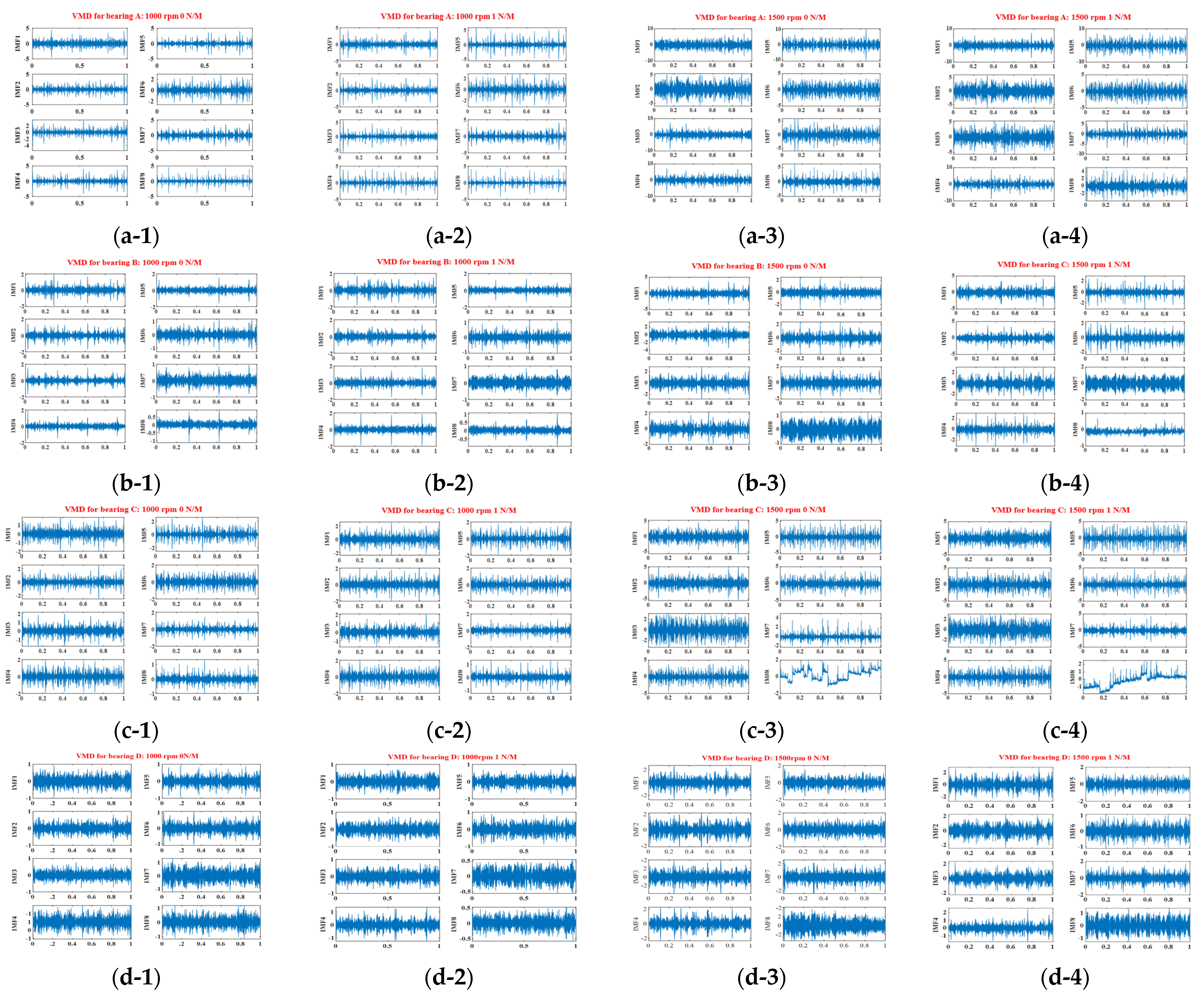
To obtain the most representative fault features, the VMD is first used to decompose the original signal. In Figure 4, eight IMFs were obtained by VMD. Based on the results, 12 signal features are calculated for each IMF, which include 10 statistical characteristics and two entropies. Therefore, 96 (12 features × 8 IMFs) fault features can be obtained from an original signal. Then, the PCA is applied to select the optimal 12 features from the original signals.

Based on optimization results, 4000 pieces of data are generated, corresponding to four working conditions of a type of bearing failure, and 1000 pieces of data are collected for each state. Then, the training dataset is randomly distributed into three sub-datasets for cross-validation. To be specific, 4000 samples of each bearing failure type are selected, where 2100 samples are used for training, 700 samples are used for validation, and others are used for testing. Finally, the final result is obtained by averaging the results of 10 cross-validations.

4.3. Feature Extraction Analysis

Referring back to the previous work, the varying operational conditions have a great influence on the signal features. It is difficult to effectively recognize the actual wearing status from simple features. Therefore, multiple appropriate features are required as the input of the classifier for training. As it is discussed above, four different wear degrees of the bearings are studied on the test-rig. According to the proposed method, the features of the vibration signal are obtained as the input of the classifier. Additionally, we proposed extra three SVM classifiers for comparison. The details of the constructed SVM models are listed as follows.

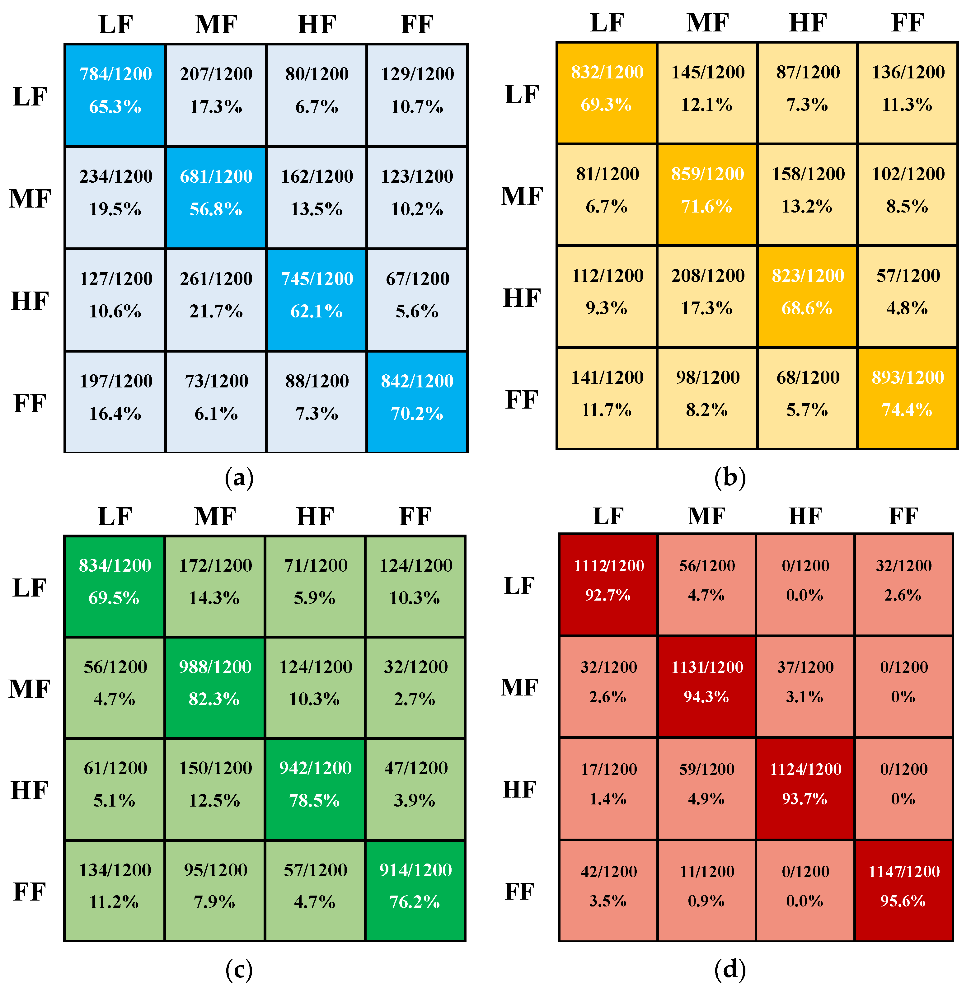
The cross-validation method is adopted for the SVM model training. To be specific, 4000 samples are selected, where 2100 samples are used for training, 700 samples are used for validation, and others are used for testing. In particular, the kernel function of SVM classifiers is a linear kernel function. The kernel function parameters and penalty coefficient are preliminarily determined by cross-verification algorithm. The characteristics of training samples are listed in

Table 4. Four different types of SVM classifiers.

Name of SVM Classifier	Characteristics of Training Samples	Number of Features
Dimensionless time domain characteristics	Mean, Peak, Kurtosis, Shape factor, Impulse factor Root mean square	6
EMD decomposition energy	Margin factor, Fuzzy entropy Sample entropy Center frequency Root variance frequency Root mean square frequency	6
VMD decomposition energy	Margin factor, Fuzzy entropy Sample entropy Center frequency Root variance frequency Root mean square frequency	6
Multi-information fusion	Mean, Peak, Kurtosis, Shape factor, Impulse factor Root mean square Margin factor, Fuzzy entropy Sample entropy Center frequency Root variance frequency Root mean square frequency	12

. In addition, Figure 5 shows the confusion matrix results of the four SVM classifiers, which represent the SF-SVM [31], EMDE-SVM [32], and VMDE-SVM [33] and our proposed BearingCog model. In these matrices, the column represents the classification attribution based on the ground truth. The sum of each column represents the total number of the class. The row in the matrix represents the actual assigned results by the classifier model. The sum of each row represents the total number of instances in this class. Observing from the confusion matrix, the main diagonal element represents the number of correctly classified samples. After calculating, the average accuracy of four SVM classifiers is shown in

Table 5. The average accuracy of recognition using different feature types.

Data Set	Different Data Feature	Recognition Accuracy Rate
Experimental data	Dimensionless time domain characteristics	63.6%
	EMD decomposition energy	71.0%
	VMD decomposition energy	76.6%
	Multi-information fusion	94.1%
CWRU data	Dimensionless time domain characteristics	75.3%
	EMD decomposition energy	84.5%
	VMD decomposition energy	90.7%
	Multi-information fusion	96.4%

. Meanwhile, it can be demonstrated that the classification efficiency of the proposed BearingCog model is obviously better than other models, which are shown in Figure 6.

In addition, to further verify the effectiveness of the proposed scheme, the datasets from Case Western Reserve University (CWRU) are introduced for analysis. The details of the defective bearing dataset are listed in

Table 6. Details of the Case Western Reserve University defective bearing dataset.

Defected Bearing	Label	Fault Diameter (mm)	Motor Load (HP)	Motor Speed (r/min)	Outer Race Data Set Position
Little fault	LF	0.1778	0	1797	OR007@6_0 (130.mat)
			1	1772	OR007@6_1 (131.mat)
Medium fault	MF	0.3556	0	1797	OR014@6_0 (197.mat)
			1	1772	OR014@6_1 (198.mat)
High fault	HF	0.5334	0	1797	OR014@6_1 (198.mat)
			1	1772	OR021@6_1 (235.mat)
Fault-free	FF	-	0	1797	Normal_0 (97.mat)
			1	1772	Normal_1 (98.mat)

. Then, the proposed method is applied to the data of CWRU, and the experimental results are shown in Table 5. In Table 5, it is obvious that the accuracy of the CWRU dataset is significantly better than the data collected by our designed test bench. The reason is due to assembly and bearing fault processing and other problems, which makes the collected data contain more background noise. However, the calculation results show that our method is superior to other methods. On the other hand, the robustness of the proposed method to noise is also demonstrated.

To further investigate the performance of these four classifiers, the receiver operating characteristic (ROC) curves are imported to depict the tradeoff relationship between the true positive rate (TPR) and the false positive rate (FPR). The definition of the TPR and FPR is listed in the Equation (9).

$$\begin{array}{l}\mathrm{FPR}=\frac{\mathrm{FP}}{\mathrm{FP}+\mathrm{TN}}\\ \mathrm{TPR}=\frac{\mathrm{TP}}{\mathrm{TP}+\mathrm{FN}}\end{array}$$

(9)

Among those, the TP represents the true positive samples. The FP represents the false positive samples. The TN represents the true negative samples. The FN represents the false negative samples. During the classification, a threshold is set appropriately to determine the predicted result. By decreasing the threshold value, more positive samples are recognized, which would raise the TPR. Oppositely, a larger threshold would assign more samples into the negative class, which would raise the FPR. Then, the area of the ROC is utilized as an effective indicator to evaluate the classifier’s performance. To be specific, if the area of the ROC is closer to 1, it represents the classifier’s model showing better robustness. In Figure 7, the areas of the SF-SVM, EMDE-SVM, VMDE-SVM, and BearingCog model is blue, green, red, and black, respectively. Based on the definition, it verifies that the proposed BearingCog is able to recognize the different fault-level bearings effectively.

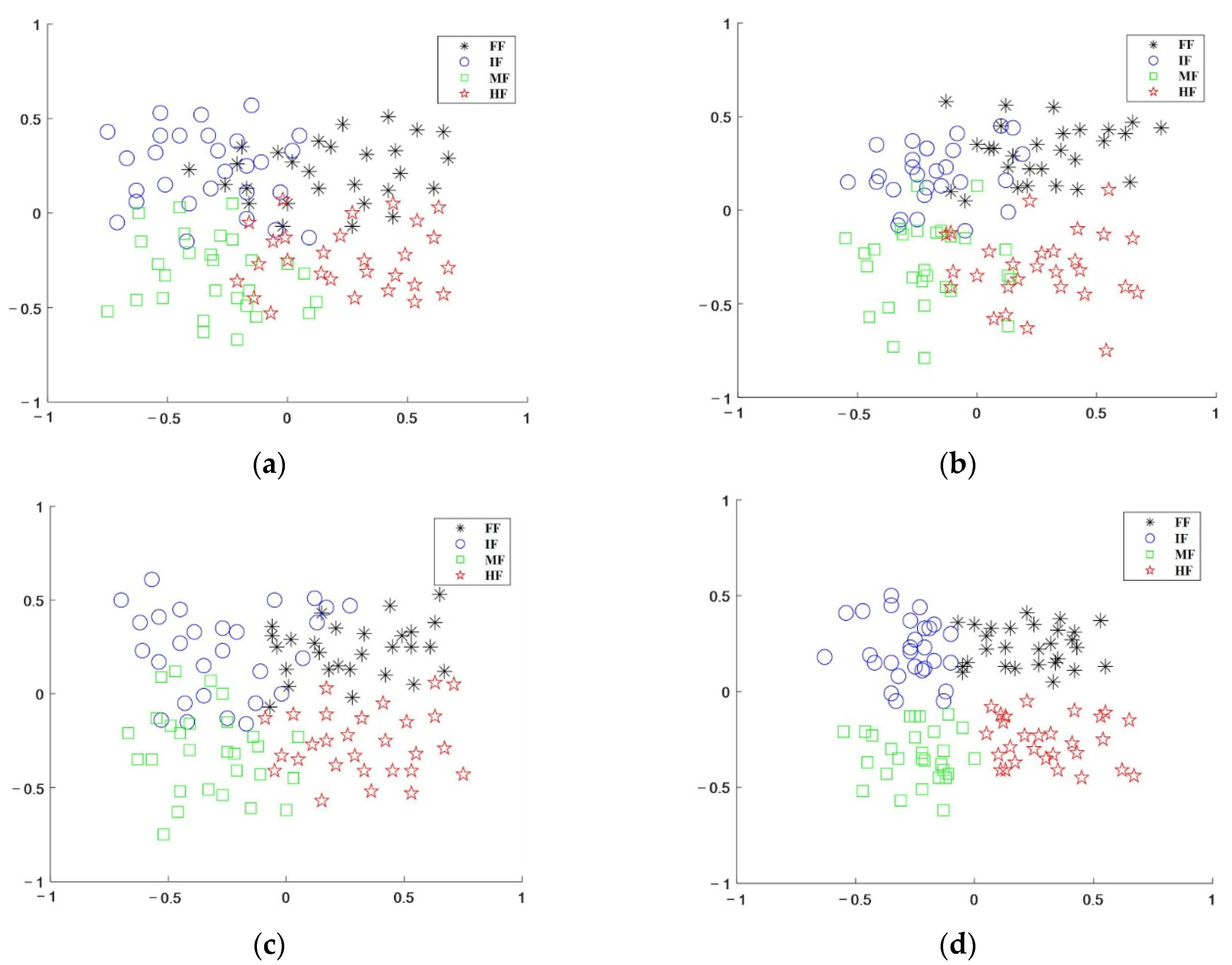
In Figure 8, to better visualize the effectiveness of the classification model, some samples are trained to demonstrate the effects of the model. Meanwhile, the t-distributed stochastic neighbor embedding is utilized to map the high-dimensional features into a two- dimensional space. It is observed that the proposed BearingCog model exhibits tighter class clustering while the other three models mix the feature distribution. It confirms that the proposed algorithm can learn more valid features and reduce the domain distribution discrepancy.

4.4. Classifier Model Optimization

To discuss the optimization of the classifier, three kernel functions, including linear kernel, polynomial kernel, and radial basis function (RBF) kernel, are imported into the SVM model for comparison. The classification results are listed in

Table 7. SVM performance results based on different kernel functions.

Bearing State	Fault Free	Little Fault	Medium Fault	High Fault
	Accuracy	Accuracy	Accuracy	Accuracy
Linear kernel	95.6%	92.7%	94.3%	93.7%
Polynomial kernel	95.7%	93.3%	94.6%	94.1%
Radial basis function kernel	96.8%	94.5%	96.7%	97.6%

. As seen from Table 7, the accuracy of the RBF kernel model is a little higher than the other two models. However, it is noted that the RBF kernel costs more training time. The reason is that the radial basis kernel function has the advantage of having fewer parameters than the polynomial kernel function. Therefore, it can simplify the complexity of the model selection.

Combined with the above analysis, the radial basis kernel function shows excellent local performance when classifying samples with close distances. Therefore, the radial basis is selected as the kernel function for the SVM multi-class classifier.

The penalty factor C amongst this is used to represent the penalty factor for the deviation, which is caused with the misclassification of samples. By adjusting the penalty factor C value, the empirical risk and confidence range can be balanced, which ensures the generalization of the classifier. To be specific, when the parameter C is large, it means that all constraints must be strictly met. It would guarantee the fitting degree of samples but decrease the generalization ability of the classifier. Conversely, when the parameter C is small, the complexity of the learning process is simplified, but the empirical risk would be increased.

Moreover, the parameter σ is used to control the gaussian distribution width of the samples. When σ is far less than the minimum distance between the training samples, all the training samples become support vectors. In other words, the classifier is over-fitting, which decreases the generalization ability of the model. Conversely, when σ is much greater than the maximum distance between the training samples, the classifier sorts all the training samples into one group. Therefore, when using the radial basis as a kernel function, the penalty factor C value and parameter σ should be carefully selected to improve both learning ability and generalization ability of the classifiers.

Inspired by this, the grid search algorithm is imported to optimize the parameter of the radial basis kernel function. The main steps are listed as follows: Firstly, an initial range and the moving step for both the parameters C and σ are given. Secondly, the SVM model is trained by moving the step of the given parameter. Then, the test result of the training classifier model is verified. As an alternative approach, the quadratic optimization strategy is imported to improve the efficiency of the searching. In detail, a large step value is first preset to obtain the rough range of optimized parameters during grid search. Then, a small step is adopted to refine the search. To ensure the efficiency and precision, it is noted that the step value is set in exponential form with a base of natural constants.

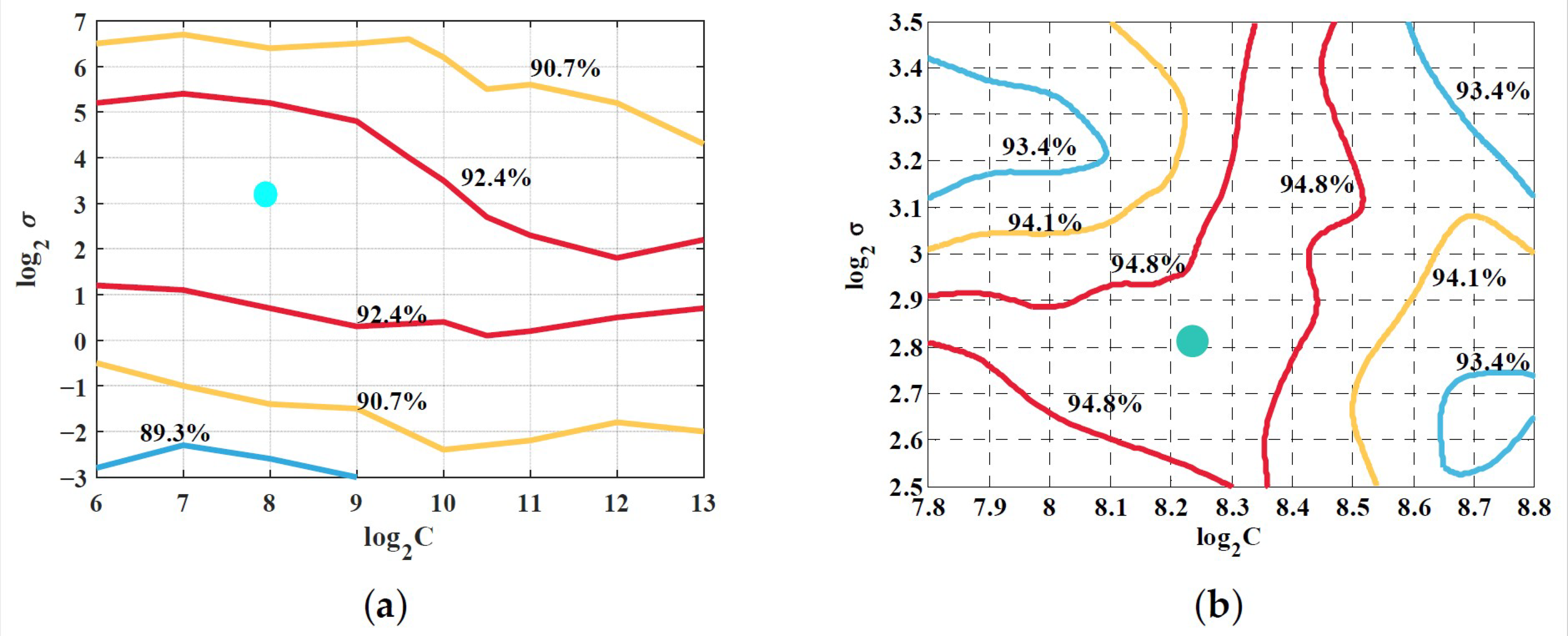
In this work, the range of the penalty factor C is set as [2⁻¹⁵, 2⁻¹⁴, 2⁻¹³,⋯, 2⁻¹,2⁰,2¹,⋯, 2¹³, 2¹⁴, 2¹⁵] while the parameter σ range is set as [2⁻⁵, 2^−4.5, 2⁻⁴,⋯, 2⁴,2^4.5,2⁵]. Then, the quadratic grid search algorithm is utilized for optimization. Figure 9a shows the contour map for the searching process. Observed from Figure 9b, the optimized point appears in (7.914, 3.297) for the first rough grid searching. Meanwhile, the classification accuracy achieves 92.4%. Based on the initial optimization results, the grids are refined, shown as Figure 10, where the optimized point appears in (8.235, 2.814). After, the optimal parameters are obtained for C = 301.2, σ = 7.03 while the classification accuracy achieves 94.8%. The experimental result shows that the grid search algorithm has achieved a better accuracy for the training model.

5. Conclusions

This article diagnosed the fault bearings under the variable operational conditions. The diagnostic conditions include varying faults, speeds, and loads. As rolling bearings rotate under variable working conditions, the vibration signals are complex. In addition, the fault features used in traditional classification models are relatively simple, which makes it difficult to identify the failure types. To improve the diagnostic accuracy, the VMD first decomposes the vibrational signal to extend the feature numbers. Then, the PCA is applied to select the optimized features, which can improve the calculation efficiency and diagnosis accuracy. Finally, the multi-information fusion training dataset is input into the SVM classifier. Moreover, the kernel function is adjusted to optimize the diagnosis accuracy of VMD. The proposed method has been successfully applied to diagnose bearing faults, and it is effective and superior to other conventional classification models. In future research activities, the bearing faults will be researched under more complex conditions, and the calculation efficiency and diagnosis accuracy will be further improved.

References

1. Liu, Z.P.; Zhang, L. A review of failure modes, condition monitoring and fault diagnosis methods for large-scale wind turbine bearings. Measurement 2020, 149, 107002–107023. [Google Scholar] [CrossRef]
2. Rai, A.; Upadhyay, S.H. A review on signal processing techniques utilized in the fault diagnosis of rolling element bearings. Tribol. Int. 2016, 96, 289–306. [Google Scholar] [CrossRef]
3. Li, X.; Zhang, W.; Din, Q. A robust intelligent fault diagnosis method for rolling element bearings based on deep distance metric learning. Neurocomputing 2018, 310, 77–95. [Google Scholar] [CrossRef]
4. Liu, R.N.; Yang, B.Y.; Zio, E.; Chen, X.F. Artificial intelligence for fault diagnosis of rotating machinery: A review. Mechanical Syst. Signal Process. 2018, 108, 33–47. [Google Scholar] [CrossRef]
5. Zhang, M.; Jiang, Z.N.; Feng, K. Research on variational mode decomposition in rolling bearings fault diagnosis of the multistage centrifugal pump. Mech. Syst. Signal Process. 2017, 93, 460–493. [Google Scholar] [CrossRef] [Green Version]
6. Liu, Z.; Zhang, L. Naturally Damaged Wind Turbine Blade Bearing Fault Detection Using Novel Iterative Nonlinear Filter and Morphological Analysis. IEEE Trans. Ind. Electron. 2020, 67, 8713–8722. [Google Scholar] [CrossRef]
7. Kong, L.; Wang, T.; Wang, P.; Zhou, Y. Research on Bearing Fault Diagnosis Method under Variable Operating Conditions Based on MWDCNN. J. Phys. Conf. Ser. 2022, 2173, 12088–12096. [Google Scholar] [CrossRef]
8. Zhao, M.; Kang, M.; Tang, B.; Pecht, M. Deep Residual Networks with Dynamically Weighted Wavelet Coefficients for Fault Diagnosis of Planetary Gearboxes. IEEE Trans. Ind. Electron. 2018, 65, 4290–4300. [Google Scholar] [CrossRef]
9. Biswal, B.; Biswal, M.; Hasan, S.; Dash, P.K. Nonstationary power signal time series data classification using LVQ classifier. Appl. Soft Comput. 2014, 18, 158–166. [Google Scholar] [CrossRef]
10. Ye, X.; Hu, Y.; Shen, J.; Chen, C.; Zhai, G. An Adaptive Optimized TVF-EMD Based on a Sparsity-Impact Measure Index for Bearing Incipient Fault Diagnosis. IEEE Trans. Instrum. Meas. 2021, 70, 1–11. [Google Scholar] [CrossRef]
11. Gao, T.; Sheng, W.; Zhou, M.; Fang, B.; Luo, F.; Li, J. Method for Fault Diagnosis of Temperature-Related MEMS Inertial Sensors by Combining Hilbert-Huang Transform and Deep Learning. Sensors 2020, 20, 5633. [Google Scholar] [CrossRef] [PubMed]
12. Wang, J.; Du, G.; Zhu, Z.; Shen, C.; He, Q. Fault diagnosis of rotating machines based on the EMD manifold. Mech. Syst. Signal Process. 2020, 135, 106443–106463. [Google Scholar] [CrossRef]
13. Fu, L.; Zhu, T.; Zhu, K.; Yang, Y. Condition Monitoring for the Roller Bearings of Wind Turbines under Variable Working Conditions Based on the Fisher Score and Permutation Entropy. Energies 2019, 12, 3085. [Google Scholar] [CrossRef] [Green Version]
14. Fu, L.; Zhu, T.; Pan, G.; Chen, S.; Zhong, Q.; Wei, Y. Power Quality Disturbance Recognition Using VMD-Based Feature Extraction and Heuristic Feature Selection. Appl. Sci. 2019, 9, 4901. [Google Scholar] [CrossRef] [Green Version]
15. Zhang, Y.; Lv, Y.; Ge, M. Complementary Ensemble Adaptive Local Iterative Filtering and Its Application to Rolling Bearing Fault Diagnosis. IEEE Access 2021, 9, 47275–47293. [Google Scholar] [CrossRef]
16. Deng, W.; Zhang, S.; Zhao, H.; Yang, X. A Novel Fault Diagnosis Method Based on Integrating Empirical Wavelet Transform and Fuzzy Entropy for Motor Bearing. IEEE Access 2018, 6, 35042–35056. [Google Scholar] [CrossRef]
17. Gao, S.; Wang, Q.; Zhang, Y. Rolling Bearing Fault Diagnosis Based on CEEMDAN and Refined Composite Multiscale Fuzzy Entropy. IEEE Trans. Instrum. Meas. 2021, 70, 1–8. [Google Scholar] [CrossRef]
18. Amar, M.; Gondal, I.; Wilson, C. Vibration Spectrum Imaging: A Novel Bearing Fault Classification Approach. IEEE Trans. Ind. Electron. 2015, 62, 494–502. [Google Scholar] [CrossRef]
19. Saidi, L.; Ben Ali, J.; Fnaiech, F. Application of higher order spectral features and support vector machines for bearing faults classification. ISA Trans. 2015, 54, 193–206. [Google Scholar] [CrossRef]
20. Lei, Y.G.; Yang, B.; Jiang, X.W.; Jia, F.; Li, N.P.; Nandi, A.K. Applications of machine learning to machine fault diagnosis: A review and roadmap. Mech. Syst. Signal Process. 2020, 138, 106587–106625. [Google Scholar] [CrossRef]
21. Shao, H.D.; Xia, M.; Han, G.J.; Zhang, Y.; Wan, J.F. Intelligent Fault Diagnosis of Rotor-Bearing System Under Varying Working Conditions with Modified Transfer Convolutional Neural Network and Thermal Images. IEEE Trans. Ind. Inform. 2021, 17, 3488–3496. [Google Scholar] [CrossRef]
22. Husari, F.; Seshadrinath, J. Incipient Interturn Fault Detection and Severity Evaluation in Electric Drive System Using Hybrid HCNN-SVM Based Model. IEEE Trans. Ind. Inform. 2022, 18, 1823–1832. [Google Scholar] [CrossRef]
23. Zhang, X.; Han, P.; Xu, L.; Zhang, F.; Wang, Y.; Gao, L. Research on Bearing Fault Diagnosis of Wind Turbine Gearbox Based on 1DCNN-PSO-SVM. IEEE Access 2020, 8, 192248–192258. [Google Scholar] [CrossRef]
24. Dragomiretskiy, K.; Zosso, D. Variational Mode Decomposition. IEEE Trans. Signal Process. 2014, 62, 531–544. [Google Scholar] [CrossRef]
25. Wang, Y.; Markert, R.; Xiang, J.; Zheng, W. Research on variational mode decomposition and its application in detecting rub-impact fault of the rotor system. Mech. Syst. Signal Process. 2015, 60–61, 243–251. [Google Scholar] [CrossRef]
26. Wang, T.; Lu, G.; Yan, P. A Novel Statistical Time-Frequency Analysis for Rotating Machine Condition Monitoring. IEEE Trans. Ind. Electron. 2020, 67, 531–541. [Google Scholar] [CrossRef]
27. Tian, J.; Morillo, C.; Azarian, M.H.; Pecht, M. Motor Bearing Fault Detection Using Spectral Kurtosis-Based Feature Extraction Coupled With K-Nearest Neighbor Distance Analysis. IEEE Trans. Ind. Electron. 2016, 63, 1793–1803. [Google Scholar] [CrossRef]
28. Lu, C.; Wang, Z.Y.; Qin, W.L.; Ma, J. Fault diagnosis of rotary machinery components using a stacked denoising autoencoder-based health state identification. Signal Process. 2017, 130, 377–388. [Google Scholar] [CrossRef]
29. Sun, W.J.; Shao, S.Y.; Zhao, R.; Yan, R.Q.; Zhang, X.W.; Chen, X.F. A sparse auto-encoder-based deep neural network approach for induction motor faults classification. Measurement 2016, 89, 171–178. [Google Scholar] [CrossRef]
30. Choudhary, A.; Goyal, D.; Letha, S.S. Infrared Thermography-Based Fault Diagnosis of Induction Motor Bearings Using Machine Learning. IEEE Sens. J. 2021, 21, 1727–1734. [Google Scholar] [CrossRef]
31. Yan, X.A.; Jia, M.P. A novel optimized SVM classification algorithm with multi-domain feature and its application to fault diagnosis of rolling bearing. Neurocomputing 2018, 313, 47–64. [Google Scholar] [CrossRef]
32. Yang, Y.; Yu, D.J.; Cheng, J.S. A fault diagnosis approach for roller bearing based on IMF envelope spectrum and SVM. Measurement 2007, 40, 943–950. [Google Scholar] [CrossRef]
33. Abdoos, A.A.; Mianaei, P.K.; Ghadikolaei, M.R. Combined VMD-SVM based feature selection method for classification of power quality events. Appl. Soft Comput. 2016, 38, 637–646. [Google Scholar] [CrossRef]
Figure 1. Main framework of the proposed BearingCog.
Applsci 12 05240 g001
Figure 2. Experimental setup for trials.
Applsci 12 05240 g002
Figure 3. Faulty bearing on the outer ring.
Applsci 12 05240 g003
Figure 4. VMD decomposition signals under different working conditions. Bearing (ad) represent little fault, medium fault, high fault, and fault-free, respectively. (a) 1 represents the torque of the load motor is set at 0 N/m under 1000 r/min. (b) 2 represents the torque of the load motor is set at 1 N/m under 1000 r/min. (c) 3 represents the torque of the load motor is set at 0 N/m under 1500 r/min. (d) 5 represents the torque of the load motor is set at 1 N/m under 1500 r/min.
Applsci 12 05240 g004
Figure 5. The confusion matrix results of the four SVM classifiers with different features. (a) SF-SVM, (b) EMDE-SVM, (c) VMDE-SVM, and (d) BearingCog-SVM.
Applsci 12 05240 g005
Figure 6. The accuracy of four kinds of SVM classifiers.
Applsci 12 05240 g006
Figure 7. The ROC curve of four kinds of SVM classifiers.
Applsci 12 05240 g007
Figure 8. The projection effect of test samples under different data feature samples: (a) based on dimensionless time domain characteristics, (b) based on EMD decomposition energy, (c) based on VMD decomposition energy, and (d) based on multi-information fusion.
Applsci 12 05240 g008
Figure 9. Parametric optimization of contour map by quadratic grid search method: (a) parameter selection for initial grid partitioning and (b) parameter selection of secondary meshing.
Applsci 12 05240 g009
Figure 10. The confusion matrix of the SVM classifier after optimization of secondary meshing parameters.
Applsci 12 05240 g010