Abstract
Assessing the condition of bridge infrastructure requires estimating damage-sensitive features from reliable sensor data. This study proposes to estimate natural frequencies from displacement measurements of a ground-based interferometric radar (GBR). These frequencies are determined from the damped vibration after each vehicle crossing with least squares and compared to a Frequency Domain Decomposition result. We successfully applied the approach in an exemplary measurement campaign at a bridge near Coburg (Germany) with an additional comparison to commonly used strain sensors. Since temperature greatly influences natural frequencies, linear regression is used to correct this influence. A simulation shows that GBR, combined with the least squares approach, achieves the lowest uncertainty and variation in the linear regression, indicating better damage detection results. However, the success of the damage detection highly depends on correctly determining the temperature influence, which might vary throughout the structure. Future work should further investigate the biases and variability of this influence.
1. Introduction
Safe operation of critical transport infrastructures, such as bridges, can only be ensured if the condition of these infrastructures is systematically assessed. A part of this assessment is analysing a bridge’s response to static or dynamic loads since structural deteriorations or damages can be indicated by a change in the response over time. The assessment of bridge infrastructure and its condition relies on various sensors and methods. For example, the output-only analysis uses accelerometers or other directly contacting sensors to measure the bridge’s response to ambient vibration from wind or vehicle traffic. Damage-sensitive features such as natural frequency or mode shapes are then estimated from the sensors’ outputs with methods based on the time or frequency domain. Over time, changes in these features can indicate damage or deterioration of the structure. However, external influences such as temperature or vehicle traffic often significantly impact the bridge’s properties. The influence can be higher than the influence expected from damage. Therefore, estimating these features with sufficient accuracy requires long-term measurements with reliable sensors.
In recent years, remote sensing techniques such as ground-based interferometric radar (GBR) have been established as an alternative to conventional sensors. GBR can measure the displacement of multiple structure points with high precision and high sampling frequency [1]. Although the measurement setup at a bridge is generally faster and less extensive with a GBR, the subsequent processing and analysis of measurement data can be more challenging than other sensors’ data. For example, the noise content of measurements mainly depends on the reflectivity of a target and external interferences, leading to considerable variation in accuracy between different measurement points of the bridge [2]. However, with some considerations to processing the GBR raw data, it is possible to receive equal or better accuracy than conventional sensors.
1.1. Related Work
Damage detection relies on the estimation of modal features of a bridge. Usually, the features are estimated from strain or acceleration measurements of the bridge’s vibration response caused by ambient excitation [3,4]. Natural frequencies are common for damage detection since they only require a few measurement points and are generally easy to estimate. However, it has been shown that the varying temperature of a structure can lead to a more significant frequency change than is expected from damage [5,6]. The relationship between temperature and natural frequency is generally linear for temperatures above freezing [7,8]. Two linear functions are applied to estimate wider temperature ranges with a discontinuity at 0 [9,10]. However, non-linear relationships are also suggested [11,12]. Besides the temperature influence, a change in natural frequency can also be observed for different traffic loads. Kim et al. [13] find a significant influence of vehicle mass for a short-span bridge. Long-span bridges show no frequency change since the ratio of vehicle mass to bridge mass is negligible. Other popular damage detection and localisation features are mode shapes and mode shape curvatures [4]. Several measurement points along the entire structure are necessary for a reliable estimation. However, unlike natural frequencies, mode shapes are not significantly affected by temperature changes or varying traffic load [8,14].
The damage-sensitive features can be estimated with parametric or non-parametric methods. A further distinction is made between time-domain and frequency-domain-based methods [15]. For example, time-domain based methods are Natural Excitation Techniques or Stochastic Subspace Identification (SSI). Peak-Picking and Frequency Domain Decomposition (FDD) are popular non-parametric methods in the frequency domain. However, parametric methods such as Least Squares Complex Frequency are also applied [15].
Finally, the estimated features can be used for damage detection. For example, changes in natural frequencies are detected with hypothesis tests after correcting for temperature-induced variance [7]. Autoregressive models can also identify frequency anomalies [9]. Analysis of changes in mode shapes or mode shape curvatures achieves an additional localisation of damage [4].
The bridge’s vibration response is usually measured with strain sensors, displacement transducers, or accelerometers (e.g., [8,9]). However, since installing these sensors can be complex and may also interrupt the regular operation of the bridge, remote sensing techniques are becoming more popular. For example, terrestrial laser scanners [16], vision-based systems [17], or GBRs [18] are used to monitor natural frequencies and mode shapes. GBR offers a very high precision while still retaining the possibility of measuring multiple points simultaneously [1,19]. It is successfully applied to determine the natural frequencies and mode shapes of buildings [20,21,22], towers [23,24], and bridges [25,26]. Natural frequencies of cables can also be identified [27,28]. The GBR results are usually validated by other sensor technology either through a direct comparison of the measurements or through a comparison of estimated modal features. A categorisation of studies, which compare and evaluate GBR with other sensor technology, is given in Table 1. For example, natural frequencies from acceleration measurements are compared to those from displacement measurements of the GBR [22,28,29,30,31]. Further comparison is achieved with mode shapes estimated from measurements of several accelerometers [32] or with the Finite Element Method (FEM) [21]. Most studies use techniques based on the frequency domain to estimate these modal features from GBR displacements. Usually, the power spectral density or the amplitude spectrum is applied for natural frequency estimation [25,31]. Mode shapes are determined through FDD [20,32] or SSI [26].

Table 1.
Related work for comparison and evaluation of ground-based radar (GBR) in the context of modal analysis. Additional sensors or models for comparison are total stations, terrestrial laser scanners (TLS), accelerometers, or the Finite Element Method (FEM).
These studies have generally found good agreement between the results of the GBR and other sensors or models. However, there is no investigation of long-term monitoring with GBR, which is relevant for determining the temperature-induced variation of natural frequencies. Additionally, the studies are usually limited to direct comparisons of estimated features without evaluating their uncertainty, which can be important for damage detection.
1.2. Objective and Contributions
Our study is motivated by the analysis of displacement measurements with GBR in the context of damage detection for bridges. We focus on output-only analysis to maintain regular bridge operation, which is a crucial advantage of remote sensors such as GBR compared to conventional sensors. Detecting deteriorations or damage to a bridge requires accurately estimating features from measurements. The success of a damage detection approach mainly depends on the uncertainty of these features. For example, it has been shown that the temperature variation of a bridge has a substantial effect on natural frequencies (e.g., [6]). Natural frequencies could not be used as features for damage detection without considering this effect. Additionally, the uncertainty of a feature also depends on the accuracy of the underlying measurements and the applied method for feature estimation. For example, natural frequencies estimated by frequency-domain methods can have insufficient resolution or may be biased by large time windows. Therefore, we propose an approach for feature estimation, which has the following objectives:
- estimation of natural frequencies from GBR measurements while accounting for the individual accuracy per measurement point;
- analysis of the influences of temperature and vehicle weight on natural frequencies;
- assessment of requirements for feature uncertainty in the context of damage detection.
In this study, we first provide a short overview of the measurement principle of GBRs to motivate the adapted approach for frequency estimation (see Section 2.1). We refer to previous studies for a more detailed description of GBRs (e.g., [1,2,18]). The measured displacements and their uncertainties are used as input data for our approach, as shown in Figure 1. After each vehicle crossing, a preprocessing step (Section 2.2.1) extracts the damped vibration. The parameters of these vibrations are then estimated in a least squares approach with a damped sinusoid model, which is described in Section 2.2.2. Since the vibrations may be disturbed by additional vehicle crossings or other influences, a test for goodness of fit filters the least squares results. The determination of test values for this test is explained in Section 2.2.3. Natural frequencies estimated with the least squares approach can be used for damage detection by testing for changes in the mean value (see Section 2.3). Section 3 shows the application of the least squares approach in a measurement campaign with a GBR and strain sensors. The results are also validated with the commonly applied Frequency Domain Decomposition (FDD). Similar to previous studies [5,6], the relationship between temperature and frequency is estimated with linear regression. Additionally, the proposed least squares approach enables a distinction between vehicle types by separately evaluating each vehicle crossing. Section 4 discusses these results in the context of damage detection with a hypothesis test. Finally, a conclusion is given in Section 5.
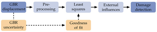
Figure 1.
Overview of the frequency estimation approach for damage detection with GBR displacements.
2. Methodology
2.1. Fundamentals of GBR
GBR determines displacements by measuring phase differences in the backscattered signal. Frequency modulation of the signal enables the distinction of multiple scattering points by their range to the GBR.Commercially available GBRs, such as IBIS-FS (IDS, Pisa, Italy), typically have a modulation bandwidth of 200 at a centre frequency of , resulting in a range resolution of . IBIS-FS achieves a sampling rate of 200 . In default operation, the GBR faces the bridge underside at an angle, as shown in Figure 2. This setup can lead to significant differences in measurement uncertainty for the bridge points. The uncertainty mainly depends on two factors. First, the scattering properties of the points determine the noise content in the backscattered signal. Lower noise content is achieved with larger reflective features, while higher noise content usually results from cluttering objects. These objects are, for example, attachments to the bridge’s underside, such as railings or pipes, which cannot be distinguished from the reflective features if they have the same range to the GBR. In general, a higher signal-to-noise ratio (SNR) directly results in higher measurement precision. The SNR results from the amplitude variation
where is the mean and is the standard deviation of the amplitude [42]. An estimate of the displacement precision results from [41]
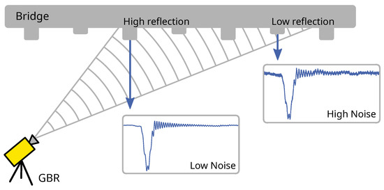
Figure 2.
Horizontal view of the measurement principle of GBR of a bridge’s underside.
Typically, a displacement precision of can be achieved with an SNR ≥ 35 dB. A second uncertainty factor is a necessary projection from the line of sight measurements to the vertical axis. The projection can lead to a significant scaling error if the actual displacement vector has more than one component [38]. However, the second factor has less relevance for determining natural frequencies. Besides reducing the measurement uncertainty through improved setups or additional processing steps, it is also important to reliably estimate this uncertainty [2]. Consideration of the uncertainty can provide valuable information in further analysis of the processed GBR measurements, for example, as input to the test for goodness of fit described in Section 2.2.3.
2.2. Least Squares for Estimation of a Damped Sinusoid
Widely used methods for estimating natural frequencies from strain or acceleration measurements are based on the frequency domain since the calculation is fast and straightforward. For example, the frequencies can be directly identified by the peaks in the power spectral density matrix. As an advancement on this principle, the Frequency Domain Decomposition (FDD) applies a Singular Value Decomposition to the spectral matrix [43]. The natural frequencies and mode shapes result from the singular values and singular vectors, respectively.
Generally, the same methods can be applied to the displacement measurements from GBR. However, we propose to use an adapted approach, which considers GBR-specific aspects. The approach estimates natural frequencies in the time domain by solving the least squares for the damped vibration after each vehicle crossing. A separate estimation of each vibration has the advantage that different measurement uncertainties of the GBR can be considered in the estimation process. Additionally, the approach does not limit the frequency resolution, as is the case for the frequency domain methods. These methods achieve sufficient frequency resolution by applying time windows with lengths in the range of minutes, therefore, aggregating several vehicle crossings in one window. With the least squares approach, it is possible to differentiate between vehicle types and analyse the estimated frequencies depending on assumed vehicle weight. A disadvantage is the need for an uninterrupted vibration after the vehicle crossing. Therefore, the proposed approach is more applicable for smaller bridges with less traffic. Then again, smaller bridges are much more affected by additional vehicle weight resulting in significant changes to the natural frequencies [13].
2.2.1. Preprocessing
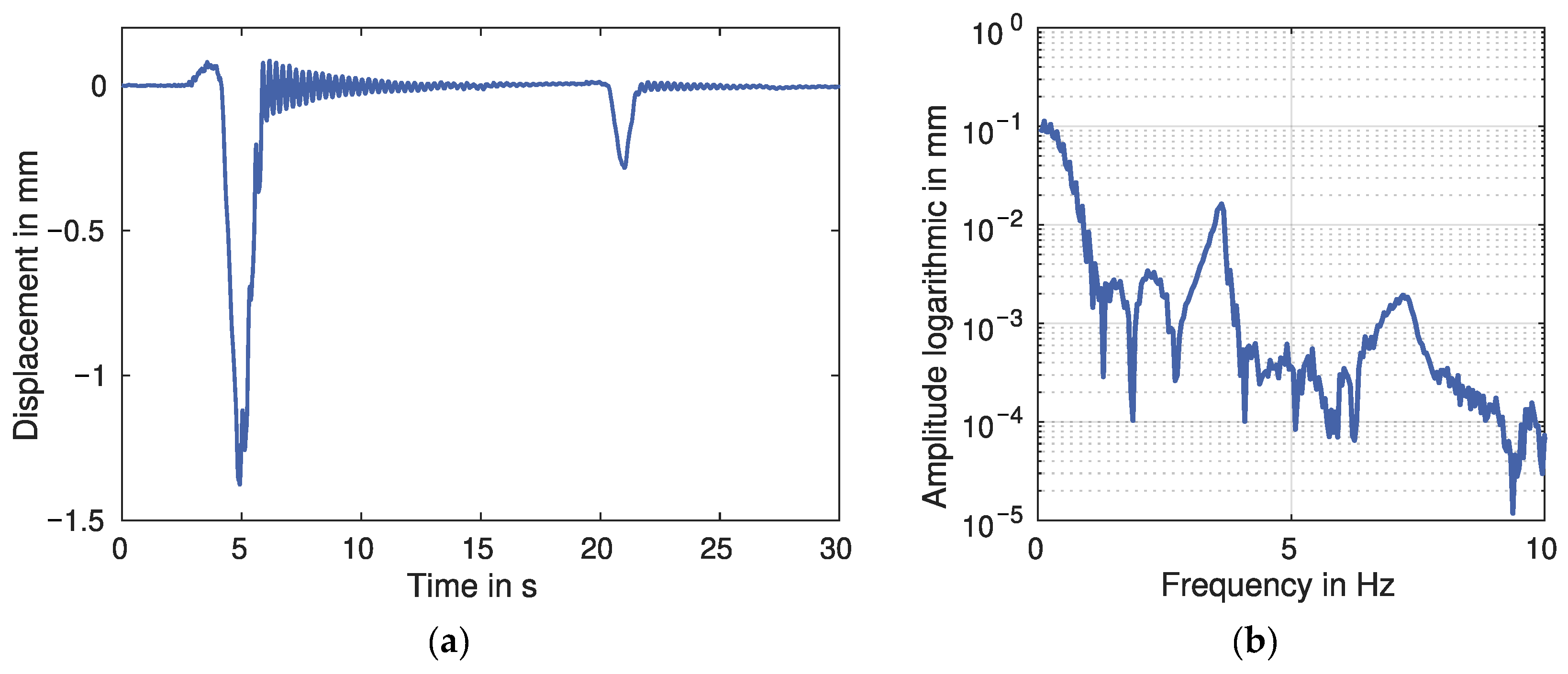
Figure 3a shows an example of typical bridge displacements measured with a GBR for two vehicle crossings. A free damped vibration follows the initial displacement caused by a vehicle. This vibration can be primarily observed in crossings of heavy vehicles, such as trucks. However, it also occurs after crossings of lighter vehicles, such as cars, although the amplitude of the vibration is much smaller. Figure 3b shows the amplitude spectrum of the displacement. The first and second natural frequencies are visible at approximately and , respectively. Generally, the amplitude of the second natural frequency is about an order of magnitude smaller than the amplitude of the first natural frequency and may be lost in the broadband noise. The proposed method is, therefore, only applied to the first natural frequency.
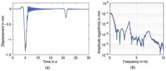
Figure 3.
Example of vehicle crossings in the time and frequency domain: (a) Bridge displacement in the time domain. (b) Amplitude spectrum of the bridge displacement.
Since the damped vibrations have recognisable characteristics in the frequency domain, their startpoints and endpoints can be detected relatively easily. A common signal processing method for detection is a bandpass filter with a passband of the first natural frequency. The vehicle crossing is then determined by applying a threshold. Alternatively, machine learning methods constitute a more complex but also more flexible approach. Combining two methods makes it possible to detect vehicle convoys, which interrupt the damped vibration [44]. After detection, a high pass filter with a cut-off frequency below the first natural frequency is applied. The filter reduces the influence of low-frequency components, which can result from short-term atmospheric disturbances to the GBR signal. Multiple scatterers in the same range cell can also cause low-frequency noise, which influences the least squares.
2.2.2. Least Squares Approach
The bridge’s response to a vehicle crossing can be modelled by a sinusoidal function with an additional damping term:
The sinusoid is defined with the natural frequency f and the phase . An enveloping exponential function determines the damping with the initial amplitude a and the decay rate . From the decay rate, the damping ratio can be determined:
A least squares approach minimises the error distances between this model and the measured displacements. Since the model is non-linear, it has to be linearised at the approximate values of the parameters. The approximate natural frequency and phase values are easiest to determine with a Discrete Fourier Transform. Although the frequency resolution is limited with the typical time window of a few seconds, the quality of the approximate values is generally high enough for the convergence of the least squares. An approximate value for the decay rate is calculated from the logarithmic decrement, which is defined as the ratio of adjoining peaks of the sinusoid:
The amplitude a can be approximated from the highest peak of the sinusoid. The approximate parameters are iteratively improved until the least squares converges.
2.2.3. Evaluation of Least Squares Estimation
The test for goodness of fit evaluates the quality of the estimated parameters. The test is necessary because additional vehicle crossings or other noise content may interrupt the damped vibration. Poor approximate values for the parameters might also cause the least squares to converge to a local minimum instead of the global minimum. The goodness of fit can be evaluated with different methods. For example, the standard error of the estimate
is calculated from the sum of squared residuals divided by the degree of freedom . If the model fits the measurement well, the standard error of the estimate should only contain broadband measurement noise. Therefore, a small difference between s and the previously estimated measurement uncertainty (see Section 2.1) indicates a good fit. Alternatively, the coefficient of determination
is defined with the sum of squared residuals divided by the sum of the squared difference between measurements and their mean value . Both approaches require a threshold to indicate a good model fit.
2.3. Damage Detection Based on a Hypothesis Test
Changes in the natural frequencies are primarily caused by varying temperatures but can also result from damage to the structure. Therefore, the results of the least squares approach can also be used to test for damage, provided that temperatures are measured, and an undamaged reference state of the bridge was previously observed. The reference measurements correct the relationship between temperature and frequency, ideally resulting in normally distributed frequencies. This correction is also applied to the test measurements to test for equality of the two distributions’ means. A significantly different mean can indicate damage to the structure. Usually, the number of reference measurements will be much higher than the number of test measurements, resulting in unequal sample sizes. It can also not be assumed that the variances of the distributions are equal because damage might influence the variance of the natural frequencies. Therefore, Welch’s t-test can be used to test for equal means. Welch’s t-test defines the test statistic T with the distributions’ means and the standard deviation s:
The standard deviation s results from the distributions’ standard deviations and sample sizes :
The test statistic is approximately t-distributed with the degree of freedom :
With a significance level , the null hypothesis of equal means is rejected under the following condition:
3. Results
We evaluate the least squares approach by applying it to several measurements at a bridge in Seßlach, Germany. The following sections show the results of the natural frequency estimation for displacement measurements by GBR in the context of damage detection.
3.1. Measurement Setup
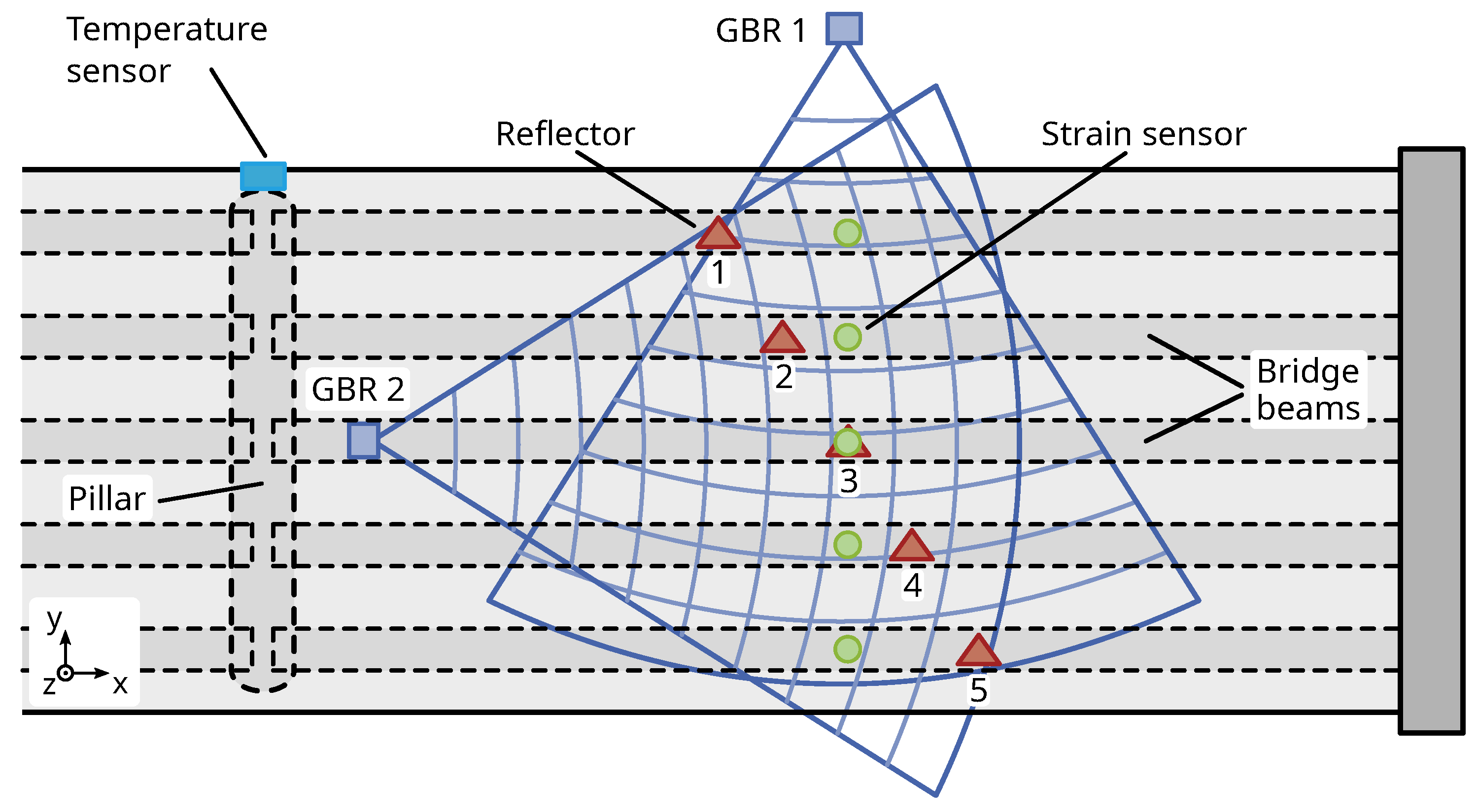
The two-span reinforced concrete bridge is part of the federal road B303 and crosses a service road in Seßlach, Germany. Each bridge field is 28 long and has five longitudinal beams. The GBR is set up orthogonally to these beams angled upwards at the bridge’s underside, as discussed in Section 2.1. This setup necessitates a projection to receive the vertical component of the displacement vector. Since the projection can be influenced by the other vector components, we apply a second GBR in line with the longitudinal beams (see also [2,38]). As a result, GBR 1 receives good signal reflection from the beams, while GBR 2 requires the installation of corner reflectors due to insufficient reflection from the smooth concrete surface (see Figure 4). Both GBRs achieve an average SNR for all measurement days of 34 dB to 40 dB for reflectors 2, 3, and 4. The average SNR for reflectors 1 and 5 is lower at 22 dB to 26 dB since the signal attenuation of the GBR antennas increases with the beam width. Consequently, the displacement precision for the vertical component varies between the reflectors. For reflectors 2, 3, and 4, the estimates range between and . The precision for reflectors 1 and 5 is estimated in the range of 0.12 to 0.29 .
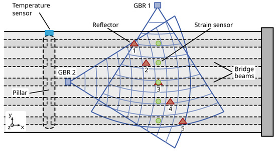
Figure 4.
Vertical view of the bridge with sensor and reflector installation.
In addition, strain sensors installed on the underside of the beams can provide reference measurements to evaluate the GBR performance for natural frequency estimation. The one-dimensional linear strain sensors from HBM (Darmstadt, Germany) have a sampling rate of 100 and their background noise during the measurements is estimated at about . Lastly, the bridge’s temperature is measured by a sensor placed on the north side of a pillar. In the following sections, we discuss the analysis of a measurement campaign with a total measurement duration of 16 . An overview of the campaign and the particular temperature ranges per day are shown in Table 2.
Table 2.
Measurement campaigns at Seßlach, Germany.
3.2. Analysis of the Relationship between Temperature and Natural Frequency
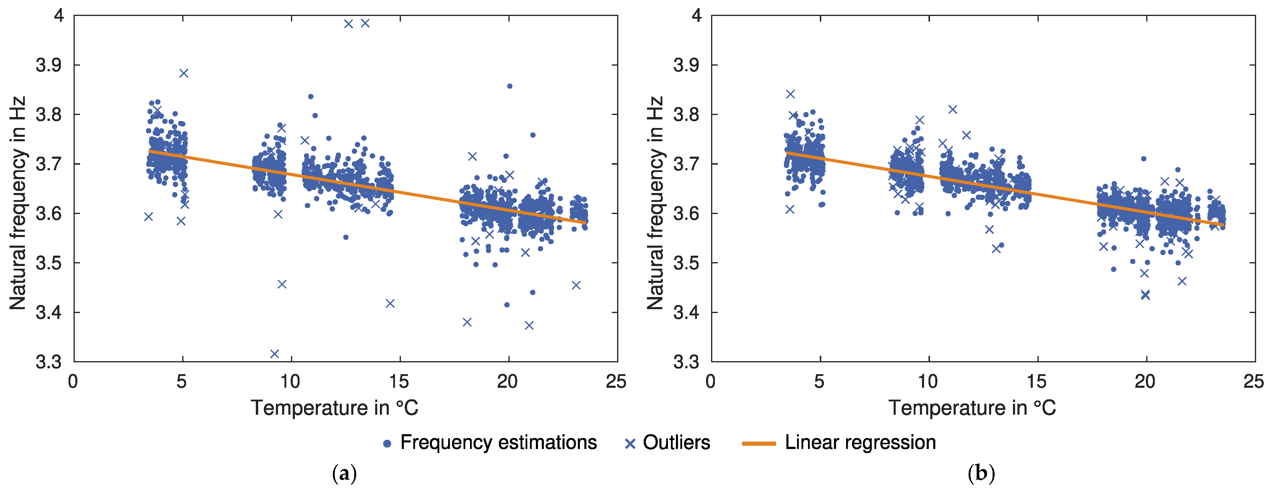
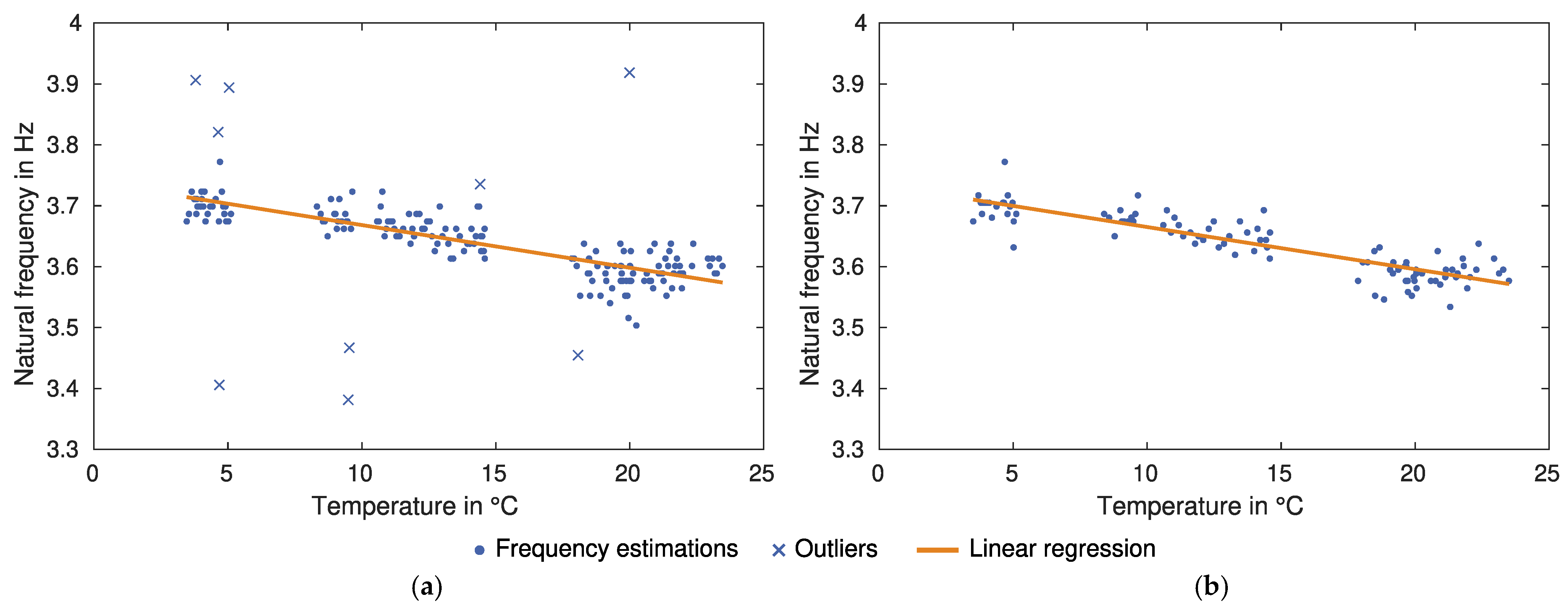
Temperature changes have a significant influence on natural frequencies, as has been shown by several studies [5,6]. Determining this influence is necessary to perform damage detection on estimated frequencies. Figure 5a shows the estimation results of the least squares approach as a function of temperature. An increase in temperature is correlated with a decrease in the first natural frequency, suggesting a linear relationship between the two values. For the Seßlach bridge, the frequencies are estimated from the GBR target with the highest SNR and thus the lowest measurement noise, which is subsequently referred to as the best approach. Outliers are marked with crosses if the test for goodness of fit falls below a threshold of 50%. Some outliers exceed the plot limits and are omitted.
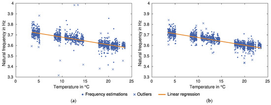
Figure 5.
Natural frequencies estimated by the least squares approach (a) from GBR measurements with the best approach and (b) from strain measurements with the mean approach.
As a direct comparison, Figure 5b shows the estimation results for the strain sensors. Contrary to the GBR data, the estimation is performed on a mean of the strain sensors’ measurements, subsequently referred to as the mean approach. The strain sensors generally have similar measurement precisions and noise content. Thus a mean of all measurements results in a higher SNR and a more stable estimation.
The linear relationship between frequency and temperature was calculated by linear regression (see Table 3). Both datasets exhibit a similar frequency change of approximately per 10 . After correcting the linear relationship, the mean value is around for both datasets. The standard deviation of the GBR’s frequency estimates is , while the strain sensors estimates result in a standard deviation of . The test for goodness of fit identifies 123 outliers for the GBR and 159 outliers for the strain sensors. Table 3 shows two additional approaches for further comparison of the GBR data. The mean approach results in 366 outliers and a standard deviation of after correcting the linear relationship. Every GBR target is individually evaluated in the single approach. About 2100 outliers were identified for this approach. After correcting for the linear relationship, the standard deviation of the frequency estimates is .
Table 3.
Comparison of natural frequency estimation for GBR and strain sensors.
3.3. Variation of the Linear Regression for Estimating the Temperature Influence
For validation of the least squares approach, we also perform Frequency Domain Decomposition (FDD) on the GBR and strain sensor measurements. Since the results are very similar between both sensor types, we will primarily be discussing the GBR results in this section. Figure 6 shows the natural frequencies as a function of temperature estimated by FDD with time windows of 5 and 10 . In the case of a time window of 5 , the resulting low-frequency resolution leads to visible quantisation. Additionally, several outliers have to be identified and removed to estimate the linear relationship between temperature and frequency successfully. We detect the outliers by iteratively testing if the residuals of the linear regression fit a normal distribution. The time window of 10 causes no visible quantisation, and only one outlier is identified. Table 4 shows the results of the linear regression. The slope parameter is approximately per 10 for both time windows. After correcting the linear relationship, the frequency estimates of the 5 time window have a standard deviation of and a mean of Hz. The results of the 10 time window are slightly lower, with a standard deviation of and a mean of .
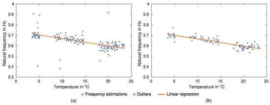
Figure 6.
Natural frequencies estimated from GBR measurements by Frequency Domain Decomposition (FDD) with (a) a time window of 5 and (b) a time window of 10 .
Table 4.
Comparison of natural frequency estimation for the least squares (LS) approach and FDD with time windows of 5 and 10 .
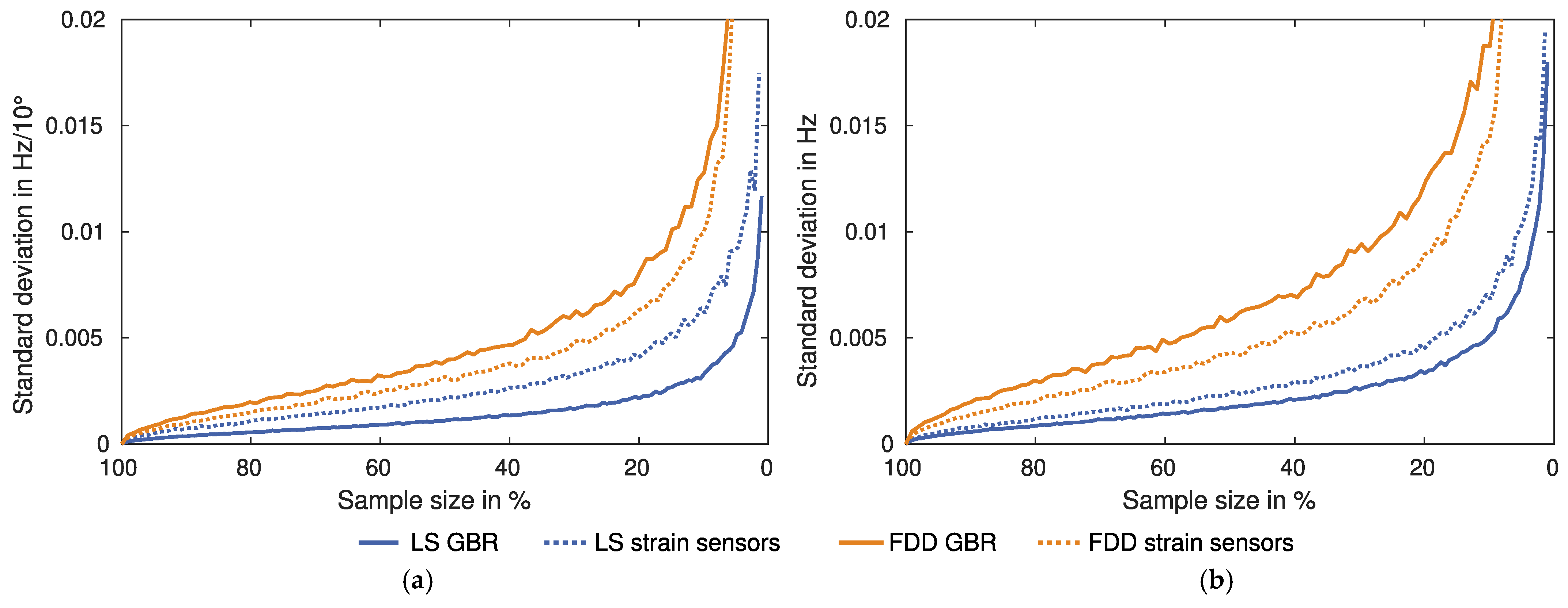
Since practical applications may require shorter measurement times or fewer campaigns, the number of frequency estimations may be reduced, thus influencing the linear regression. In the following, we analyse the reliability of the linear regression by simulating two types of data reductions. At first, the reduction is implemented by drawing uniformly distributed random samples from the least squares and FDD results, respectively. Figure 7 shows the variation of the linear regression’s parameters calculated from one thousand samples for each sample size. The standard deviation of the slope parameter in Figure 7a slowly increases as the sample size is reduced. With very small sample sizes, the growth can be characterised as exponential. The standard deviation is continually smaller for the least squares result than it is for the FDD. Although this difference can be observed for both the GBR and the strain sensors, it is much more distinct for the GBR. Figure 7b shows very similar observations for the offset parameter of the linear regression.
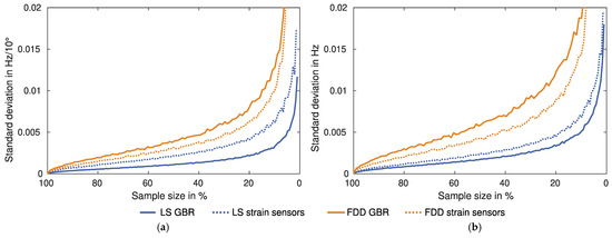
Figure 7.
Variation of the linear regression depending on sample size. The least squares (LS) uses the best approach for GBR and the mean approach for the strain sensors. The FDD has a time window of 10 : (a) Variation of slope parameter. (b) Variation of offset parameter.
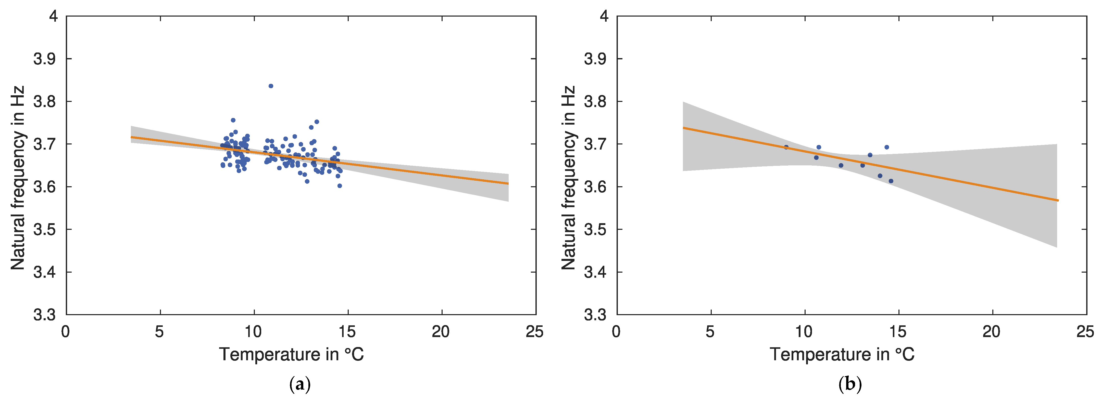
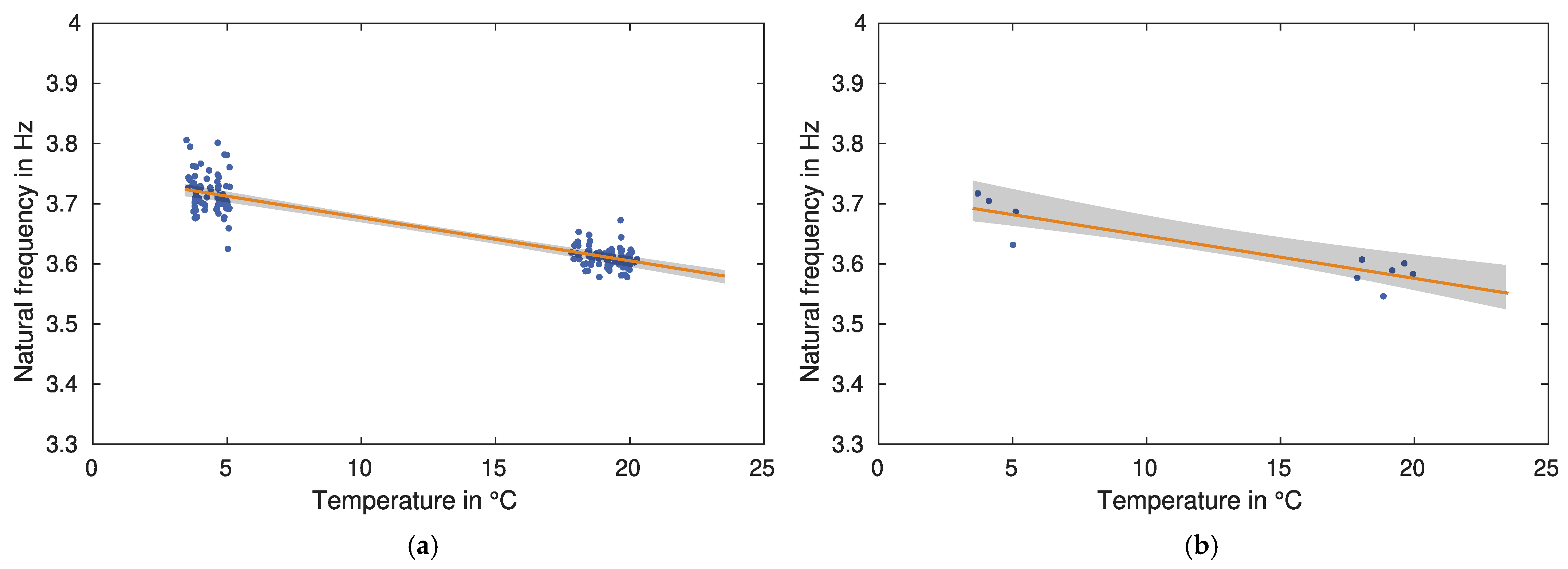
A second simulation excludes entire measurement days combined with uniformly distributed random samples. Figure 8 exemplarily shows the variation of the linear regression for a sample size of 25%. The measurement days only include the 23 and 24 October 2019, with temperatures in the range of 8 to 15 . The samples are drawn one thousand times from the GBR least squares result to visualise the standard deviation of the linear regression in Figure 8a. Additionally, one sample and its corresponding regression are plotted to illustrate the data reduction. As a direct comparison, Figure 8b shows the FDD result with a time window of 10 for this simulation. The standard deviation of the linear regression is much higher for the FDD than for the least squares approach, especially in the case of extrapolated values outside the reduced temperature range. A similar result can be seen in Figure 9. The simulation uses two measurement days with a greater differential between lowest and highest temperatures than the first simulation. Temperatures are between 3 and 6 on 27 February 2020 and between 17 and 21 on 29 July 2020. As a result, the linear regression varies much less for the least squares approach and the FDD than in the previous simulation. However, the FDD still has a higher standard deviation than the least squares approach.
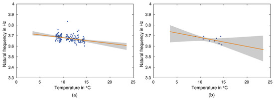
Figure 8.
Variation of the linear regression with GBR data for a sample size of 25% and a reduction of the measurement days to the 23 and 24 October 2019: (a) Least squares with best approach. (b) FDD with a time window of 10 .
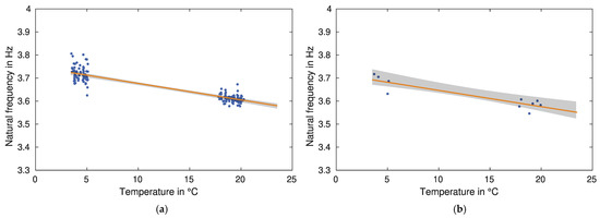
Figure 9.
Variation of the linear regression with GBR data for a sample size of 25% and a reduction of the measurement days to the 27 February 2020 and 29 July 2020: (a) Least squares with best approach. (b) FDD with a time window of 10 .
3.4. Influence of Vehicle Types on Natural Frequencies
Since the least squares approach estimates frequencies from the damped vibration after a vehicle crossing, a separate analysis of different vehicle types and their influence on the first natural frequency is possible. Vehicle types can be distinguished by the peak displacement during a crossing since the displacement is approximately proportional to the vehicle’s weight. In the following, we only differentiate between two major types of vehicles. Light vehicles have an absolute peak displacement of smaller than and include cars, vans, and small trucks. Accordingly, heavy vehicles, such as trucks or trucks with trailers, are characterised by an absolute peak displacement higher than . The threshold is certainly chosen arbitrarily and may only be a rough characterisation of the suggested vehicle types. However, Table 5 clearly shows an influence on natural frequency estimation. After correcting the linear relationship of frequency and temperature with linear regression, the heavy vehicles have a lower frequency mean than the light vehicles by about . The slope of the regression and the standard deviation are approximately similar. For the strain measurements, a comparable distinction between light and heavy vehicles can be achieved with a threshold of 6 . Table 5 shows a difference in the frequency mean of between the vehicle types. Furthermore, the standard deviation increases to for heavy vehicles and decreases to for light vehicles.
Table 5.
Comparison of vehicle types for natural frequency estimation with GBR measurements analysed by the best approach. In the case of GBR, vehicles are characterised by the absolute of the peak displacement: heavy vehicles > , light vehicles < . In the case of the strain sensors, vehicles are characterised by the peak strain: heavy vehicles > 6 , light vehicles < 6 .
3.5. Simulation of Damage Detection
After correcting the temperature influence, a hypothesis test can detect a change in the frequencies’ mean. In this section, we illustrate the necessary properties of the test to detect a change in the previously estimated frequencies. A simulation of a test measurement can indicate the required minimum difference between the test distribution and the reference distribution. We assume that the test distribution consists of frequency estimations from 30 of measurements with a standard deviation equal to the reference distribution. Furthermore, both distributions are normally distributed, and the significance level is defined as 5%. The least squares approach with GBR measurements would result in approximately 50 frequency estimations and a minimum detectable difference of 8 . The FDD with a 5 window generates six frequency estimations resulting in a difference of 27 . In the case of the strain sensors’ result, the required difference is 13 for the least squares approach.
4. Discussion
The measurements at the bridge in Seßlach (Germany) confirm the temperature-induced change of the first natural frequency as it has already been shown by other studies (e.g., [5,6]). At first, we discuss the results for estimating this relationship with the proposed least squares approach. The approach is then compared to the FDD and examined in the context of damage detection.
4.1. Comparison of GBR and Strain Sensors
The approach is able to determine natural frequencies from GBR displacement measurements as well as from strain measurements. Generally, the approach benefits from measurements with high SNR resulting in a smaller variation of the frequency estimations and fewer outliers. In the case of the strain sensors, the highest SNR is achieved by averaging all measurements in the mean approach. Since the sensors have a similar noise level and the noise is uncorrelated, averaging reduces the noise power by a factor of N, where N is the number of sensors. In the case of GBR, the best approach uses the measurement of the target with the highest SNR, which results in the lowest standard deviation and fewest outliers for the frequency estimations. Averaging multiple targets does not increase the SNR compared to the target with the best SNR. One cause for this is the significant difference in signal reflection for the GBR targets, which leads to dissimilar SNRs (see Section 2.1). Secondly, the sensor noise as part of the overall noise level may be correlated between targets. A comparison of the two sensors shows very similar results for the linear regression. After correcting the linear relationship, the GBR achieves a smaller standard deviation than the strain sensors. This difference can be explained by the higher SNR for the GBR, even though the noise level for the strain sensors is improved by averaging. The strain sensors’ result still has some undetected outliers influencing the standard deviation. Choosing a threshold for the goodness of fit is always a compromise between the number of false positives and false negatives. A threshold of reduces the number of false negatives to improve the reliability of the linear regression. The resulting higher number of false positives is acceptable since the remaining number of frequency estimations is still very high. We use the same threshold for both sensors to achieve a direct comparison. However, the strain sensors can reach a comparable standard deviation to the GBR if a higher threshold of is used. Generally, the number of outliers for both sensors shows the importance of the test for goodness of fit, which is necessary to achieve a reliable linear regression.
4.2. Comparison of Least Squares and FDD
After comparing the two sensor types, the least squares approach is evaluated against the FDD. Both methods generally result in very similar linear regressions. However, the frequency mean is slightly lower when calculated by the FDD. This difference is caused by the large time window of several minutes, which contains multiple vehicle crossings. Most importantly, the time window also includes the crossing itself with the added weight of the vehicle. For small bridges, the added weight significantly lowers the natural frequency, which is observed indirectly through the averaging effect of the FDD. Another effect of the time window is the significantly lower number of frequency estimations compared to the least squares approach. This effect causes more significant variation in the linear regression, as shown in Figure 7, Figure 8 and Figure 9. The simulations demonstrate that the least squares approach allows shorter measurements and a narrower temperature band than the FDD. For example, a real-world monitoring scenario could be constructed with only one measurement during the summer and one during the winter. The resulting temperature range would be sufficient to estimate the linear relationship with the least squares approach and perform damage detection on new measurements. However, it is important to note that the simulations only provide qualitative comparisons between the two methods and cannot assess the accuracy of the linear regression itself. For example, biases caused by an unequal temperature distribution are not considered since the temperature is measured at only one location on the exterior of the structure.
4.3. Influence of Vehicle Types on Natural Frequencies
Since the least squares approach estimates the frequency for every vehicle crossing separately, we can further distinguish between heavy and light vehicles. Even though the approach only uses the damped vibration after a vehicle has already left the bridge, a difference between the two types can still be determined. The difference in the frequency mean is likely to result from a residual influence of the lower natural frequency during the vehicle crossing. A residual influence of the excitation frequency is also possible. The difference could become relevant for damage detection if the vehicle type distribution significantly changes between consecutive measurements. For example, a (temporary) diversion of heavy vehicles to or from the monitored bridge could possibly induce a significant frequency change detectable with a hypothesis test. If the change in the vehicle type’s distribution is not noticed, the frequency change could be misinterpreted as damage to the structure. The difference in the frequency mean is comparably determined from both the GBR’s result and the strain sensors’ result. However, the standard deviation changes significantly between vehicle types for the strain sensors, which is not observed for the GBR. The higher standard deviation for heavy vehicles results from outliers, which are not detected by the test for goodness of fit. As discussed before, with a higher threshold, the strain sensors can achieve comparable results to the GBR.
4.4. Hypothesis Test for Damage Detection
The simulation of the hypothesis test for damage detection shows that minimal changes in the frequencies’ mean can be detected. However, the discussed values for the minimum difference should only be interpreted as a qualitative comparison between the sensors and methods. Biases in temperature or skewed distributions could significantly influence the test leading to much higher required differences. Since the test mainly depends on the standard deviations of the distributions, the strain sensors’ result requires a higher difference than the GBR’s result. However, the test also leads to a higher difference if the number of elements in the test distribution decreases. The few elements in the FDD’s test distribution result in a much higher value, indicating that longer measurement times are required for this method.
5. Conclusions and Outlook
This study discusses the estimation of natural frequencies from GBR displacement measurements by a least squares approach. The approach fits the model of a damped sinusoid to the vibration after a vehicle crossing. With the additional test for goodness of fit, we are able to reliably estimate the linear relationship between the first natural frequency and temperature. Compared to strain sensors, the GBR results have a lower standard deviation and fewer outliers, which benefits the detection of frequency changes caused by damage to the bridge. The least squares approach is also validated with the Frequency Domain Decomposition. While both methods obtain very similar results, the linear regression for determining the relationship between temperature and frequency is more stable in the case of the least squares approach. The approach can better tolerate a simulated reduction of measurement time than the FDD, especially if entire temperature ranges are omitted. It is also possible to separate the vehicle crossings into two different weight classes. Heavy vehicles lead to a lower frequency mean even though the analysed vibration occurs after a vehicle has already left the bridge. Frequency changes beyond the temperature influence can be detected with a hypothesis test, enabling a reliable damage detection approach.
Since the least squares approach ideally requires uninterrupted damped vibrations, it is only applicable to smaller bridges with a higher likelihood of singular vehicle crossings. Additionally, it has only been tested for the first natural frequency. In future work, we aim to determine the second natural frequency, which should be possible considering the accuracy of GBR. With additional targets, it is also possible to determine mode shapes, which can be used for damage detection and localisation. Considering the substantial influence of temperature change to natural frequencies, further study on the variability of temperatures throughout the structure would benefit the reliability of damage detection.
Author Contributions
All authors prepared the methodological concept of this study, the original draft, as well as the editing of the manuscript. C.M. designed the software, curated the data, and performed the investigation, formal analysis, and validation. All authors contributed to the visualization of the data and results. S.K. initialized the related research and provided didactic and methodological inputs. All authors have read and agreed to the published version of the manuscript.
Funding
This work is part of the project ZEBBRA, funded by the German Ministry for Education and Research (BMBF).
Data Availability Statement
The data are not publicly available as they contain sensitive information about the investigated bridge structure.
Acknowledgments
We thank Matthias Arnold, Andreas Döring, and the Büro für Strukturmechanik for supporting the measurements. We also thank Stefan Hinz for his support. We acknowledge support by the KIT-Publication Fund of the Karlsruhe Institute of Technology.
Conflicts of Interest
The authors declare no conflict of interest.
References
- Gentile, C.; Bernardini, G. An interferometric radar for non-contact measurement of deflections on civil engineering structures: Laboratory and full-scale tests. Struct. Infrastruct. Eng. 2009, 6, 521–534. [Google Scholar] [CrossRef]
- Michel, C.; Keller, S. Advancing Ground-Based Radar Processing for Bridge Infrastructure Monitoring. Sensors 2021, 21, 2172. [Google Scholar] [CrossRef] [PubMed]
- Moughty, J.J.; Casas, J.R. A State of the Art Review of Modal-Based Damage Detection in Bridges: Development, Challenges, and Solutions. Appl. Sci. 2017, 7, 510. [Google Scholar] [CrossRef] [Green Version]
- Fan, W.; Qiao, P. Vibration-based Damage Identification Methods: A Review and Comparative Study. Struct. Health Monit. 2010, 10, 83–111. [Google Scholar] [CrossRef]
- Sohn, H. Effects of environmental and operational variability on structural health monitoring. Philos. Trans. R. Soc. A Math. Phys. Eng. Sci. 2006, 365, 539–560. [Google Scholar] [CrossRef]
- Han, Q.; Ma, Q.; Xu, J.; Liu, M. Structural health monitoring research under varying temperature condition: A review. J. Civ. Struct. Health Monit. 2020, 11, 149–173. [Google Scholar] [CrossRef]
- Liu, C.; DeWolf, J.T. Effect of Temperature on Modal Variability of a Curved Concrete Bridge under Ambient Loads. J. Struct. Eng. 2007, 133, 1742–1751. [Google Scholar] [CrossRef]
- Anastasopoulos, D.; Roeck, G.D.; Reynders, E.P.B. One-year operational modal analysis of a steel bridge from high-resolution macrostrain monitoring: Influence of temperature vs. retrofitting. Mech. Syst. Signal Process. 2021, 161, 107951. [Google Scholar] [CrossRef]
- Peeters, B.; Roeck, G.D. One-year monitoring of the Z24-Bridge: Environmental effects versus damage events. Earthq. Eng. Struct. Dyn. 2001, 30, 149–171. [Google Scholar] [CrossRef]
- Jin, C.; Li, J.; Jang, S.; Sun, X.; Christenson, R. Structural damage detection for in-service highway bridge under operational and environmental variability. In Sensors and Smart Structures Technologies for Civil, Mechanical, and Aerospace Systems; Lynch, J.P., Ed.; SPIE: Bellingham, WA, USA, 2015. [Google Scholar] [CrossRef]
- Ding, Y.; Li, A. Temperature-induced variations of measured modal frequencies of steel box girder for a long-span suspension bridge. Int. J. Steel Struct. 2011, 11, 145–155. [Google Scholar] [CrossRef]
- Ni, Y.Q.; Hua, X.G.; Fan, K.Q.; Ko, J.M. Correlating modal properties with temperature using long-term monitoring data and support vector machine technique. Eng. Struct. 2005, 27, 1762–1773. [Google Scholar] [CrossRef]
- Kim, C.Y.; Yoon, N.S.K.J.G.; Jung, D.S. Effect of Vehicle Mass on the Measured Dynamic Characteristics of Bridges from Traffic-Induced Vibration Test. In Proceedings of SPIE The International Society of Optical Engineering; International Society for Optical Engineering: Bellingham, WA, USA, 2001. [Google Scholar]
- Zhang, Q.W.; Fan, L.C.; Yuan, W.C. Traffic-induced variability in dynamic properties of cable-stayed bridge. Earthq. Eng. Struct. Dyn. 2002, 31, 2015–2021. [Google Scholar] [CrossRef]
- Rainieri, C.; Fabbrocino, G. Operational Modal Analysis of Civil Engineering Structures; Springer: New York, NY, USA, 2014. [Google Scholar] [CrossRef]
- Artese, S.; Nico, G. TLS and GB-RAR Measurements of Vibration Frequencies and Oscillation Amplitudes of Tall Structures: An Application to Wind Towers. Appl. Sci. 2020, 10, 2237. [Google Scholar] [CrossRef] [Green Version]
- Zona, A. Vision-Based Vibration Monitoring of Structures and Infrastructures: An Overview of Recent Applications. Infrastructures 2020, 6, 4. [Google Scholar] [CrossRef]
- Pieraccini, M.; Miccinesi, L. Ground-Based Radar Interferometry: A Bibliographic Review. Remote Sens. 2019, 11, 1029. [Google Scholar] [CrossRef] [Green Version]
- Xing, C.; Yu, Z.Q.; Zhou, X.; Wang, P. Research on the Testing Methods for IBIS-S System. IOP Conf. Ser. Earth Environ. Sci. 2014, 17, 012263. [Google Scholar] [CrossRef] [Green Version]
- Hu, J.; Guo, J.; Zhou, L.; Zhang, S.; Chen, M.; Hang, C. Dynamic Vibration Characteristics Monitoring of High-Rise Buildings by Interferometric Real-Aperture Radar Technique: Laboratory and Full-Scale Tests. IEEE Sens. J. 2018, 18, 6423–6431. [Google Scholar] [CrossRef]
- Negulescu, C.; Luzi, G.; Crosetto, M.; Raucoules, D.; Roullé, A.; Monfort, D.; Pujades, L.; Colas, B.; Dewez, T. Comparison of seismometer and radar measurements for the modal identification of civil engineering structures. Eng. Struct. 2013, 51, 10–22. [Google Scholar] [CrossRef]
- Alva, R.E.; Pujades, L.G.; González-Drigo, R.; Luzi, G.; Caselles, O.; Pinzón, L.A. Dynamic Monitoring of a Mid-Rise Building by Real-Aperture Radar Interferometer: Advantages and Limitations. Remote Sens. 2020, 12, 1025. [Google Scholar] [CrossRef] [Green Version]
- Atzeni, C.; Bicci, A.; Dei, D.; Fratini, M.; Pieraccini, M. Remote Survey of the Leaning Tower of Pisa by Interferometric Sensing. IEEE Geosci. Remote Sens. Lett. 2010, 7, 185–189. [Google Scholar] [CrossRef]
- Nico, G.; Prezioso, G.; Masci, O.; Artese, S. Dynamic Modal Identification of Telecommunication Towers Using Ground Based Radar Interferometry. Remote Sens. 2020, 12, 1211. [Google Scholar] [CrossRef] [Green Version]
- Luzi, G.; Crosetto, M.; Fernández, E. Radar Interferometry for Monitoring the Vibration Characteristics of Buildings and Civil Structures: Recent Case Studies in Spain. Sensors 2017, 17, 669. [Google Scholar] [CrossRef] [PubMed] [Green Version]
- Liu, X.; Zhao, S.; Wang, P.; Wang, R.; Huang, M. Improved Data-Driven Stochastic Subspace Identification with Autocorrelation Matrix Modal Order Estimation for Bridge Modal Parameter Extraction Using GB-SAR Data. Buildings 2022, 12, 253. [Google Scholar] [CrossRef]
- Wang, J.; Wang, X.; Fan, C.; Li, Y.; Huang, X. Bridge Dynamic Cable-Tension Estimation with Interferometric Radar and APES-Based Time-Frequency Analysis. Electronics 2021, 10, 501. [Google Scholar] [CrossRef]
- Gentile, C. Application of Microwave Remote Sensing to Dynamic Testing of Stay-Cables. Remote Sens. 2009, 2, 36–51. [Google Scholar] [CrossRef] [Green Version]
- Erdélyi, J.; Kopáčik, A.; Kyrinovič, P. Spatial Data Analysis for Deformation Monitoring of Bridge Structures. Appl. Sci. 2020, 10, 8731. [Google Scholar] [CrossRef]
- Farrar, C.; Darling, T.; Migliori, A.; Baker, W. Microwave interferometers for non-contact vibration measurements on large structures. Mech. Syst. Signal Process. 1999, 13, 241–253. [Google Scholar] [CrossRef] [Green Version]
- Sofi, M.; Lumantarna, E.; Mendis, P.A.; Duffield, C.; Rajabifard, A. Assessment of a Pedestrian Bridge Dynamics Using Interferometric Radar System IBIS-FS. Procedia Eng. 2017, 188, 33–40. [Google Scholar] [CrossRef]
- Gentile, C.; Bernardini, G. Output-only modal identification of a reinforced concrete bridge from radar-based measurements. NDT E Int. 2008, 41, 544–553. [Google Scholar] [CrossRef]
- Alani, A.M.; Aboutalebi, M.; Kilic, G. Use of non-contact sensors (IBIS-S) and finite element methods in the assessment of bridge deck structures. Struct. Concr. 2014, 15, 240–247. [Google Scholar] [CrossRef]
- Kuras, P.; Ortyl, Ł.; Owerko, T.; Salamak, M.; Łaziński, P. GB-SAR in the Diagnosis of Critical City Infrastructure—A Case Study of a Load Test on the Long Tram Extradosed Bridge. Remote Sens. 2020, 12, 3361. [Google Scholar] [CrossRef]
- Pieraccini, M.; Parrini, F.; Fratini, M.; Atzeni, C.; Spinelli, P. In-service testing of wind turbine towers using a microwave sensor. Renew. Energy 2008, 33, 13–21. [Google Scholar] [CrossRef]
- Castellano, A.; Fraddosio, A.; Martorano, F.; Mininno, G.; Paparella, F.; Piccioni, M.D. Structural health monitoring of a historic masonry bell tower by radar interferometric measurements. In Proceedings of the 2018 IEEE Workshop on Environmental, Energy, and Structural Monitoring Systems (EESMS), Salerno, Italy, 21–22 June 2018. [Google Scholar] [CrossRef]
- Diaferio, M.; Fraddosio, A.; Piccioni, M.D.; Castellano, A.; Mangialardi, L.; Soria, L. Some issues in the structural health monitoring of a railway viaduct by ground based radar interferometry. In Proceedings of the 2017 IEEE Workshop on Environmental, Energy, and Structural Monitoring Systems (EESMS), Milan, Italy, 24–25 July 2017. [Google Scholar] [CrossRef]
- Miccinesi, L.; Beni, A.; Pieraccini, M. Multi-Monostatic Interferometric Radar for Bridge Monitoring. Electronics 2021, 10, 247. [Google Scholar] [CrossRef]
- Firus, A.; Schneider, J.; Becker, M.; Pullamthara, J.J.; Grunert, G. Microwave Interferometry Measurements for Railway-specific Applications. In Proceedings of the 6th International Conference on Computational Methods in Structural Dynamics and Earthquake Engineering (COMPDYN 2015), Rhodes Island, Greece, 15–17 June 2017. [Google Scholar] [CrossRef]
- Neitzel, F.; Niemeier, W.; Weisbrich, S.; Lehmann, M. Investigation of low-cost accelerometer, terrestrial laser scanner and ground-based radar interferometer for vibration monitoring of bridges. In Proceedings of the 6th European Workshop on Structural Health Monitoring 2012, Dresden, Germany, 3–6 July 2012; Volume 1, pp. 542–551. [Google Scholar]
- Rödelsperger, S.; Läufer, G.; Gerstenecker, C.; Becker, M. Monitoring of displacements with ground-based microwave interferometry: IBIS-S and IBIS-L. J. Appl. Geod. 2010, 4, 41–54. [Google Scholar] [CrossRef]
- Coppi, F.; Gentile, C.; Ricci, P.P.; Tomasini, E.P. A Software Tool for Processing the Displacement Time Series Extracted from Raw Radar Data. In AIP Conference Proceedings; AIP: College Park, MD, USA, 2010. [Google Scholar] [CrossRef]
- Brincker, R.; Zhang, L.; Andersen, P. Modal Identification from Ambient Responses using Frequency Domain Decomposition. In Proceedings of the International Modal Analysis Conference (IMAC), San Antonio, TX, USA, 7–10 February 2000; pp. 625–630. [Google Scholar]
- Arnold, M.; Hoyer, M.; Keller, S. Convolutional Neural Networks For Detecting Bridge Crossing Events With Ground-Based Interferometric Radar Data. ISPRS Ann. Photogramm. Remote Sens. Spat. Inf. Sci. 2021, V-1-2021, 31–38. [Google Scholar] [CrossRef]


Publisher’s Note: MDPI stays neutral with regard to jurisdictional claims in published maps and institutional affiliations. |
© 2022 by the authors. Licensee MDPI, Basel, Switzerland. This article is an open access article distributed under the terms and conditions of the Creative Commons Attribution (CC BY) license (https://creativecommons.org/licenses/by/4.0/).