Article

Reportability Tool Design: Assessing Grouping Schemes for Strategic Decision Making in Maintenance Planning from a Stochastic Perspective

by
Pablo Viveros
*,
Nicolás Cárdenas Pantoja
,
Fredy Kristjanpoller
and
Rodrigo Mena
Department of Industrial Engineering, Universidad Técnica Federico Santa María, Valparaíso 2340000, Chile
*
Author to whom correspondence should be addressed.
Appl. Sci. 2022, 12(11), 5386; https://doi.org/10.3390/app12115386
Submission received: 18 April 2022 / Revised: 11 May 2022 / Accepted: 22 May 2022 / Published: 26 May 2022
(This article belongs to the Special Issue Reliability Modelling and Analysis for Complex Systems, Volume 2)

Abstract

:

Featured Application

The aim of the following work is to provide a reportability tool designed in Power BI addressing risk and performance of maintenance activity scheduling from a strategic and stochastic perspective.

Abstract

In this article, we report on the design and implementation of a reportability tool using Microsoft Power BI embedded with Python script to assess opportunistic grouping schemes under a preventive maintenance policy. The reportability tool is based on specially developed indicators based on current maintenance standards for better implementation and considers a formerly developed grouping strategy with poor embedded performance indicators as an implementation case for the tool. Performance indicators were carefully developed considering a stochastic perspective when possible; this enables decisions to be influenced by risk assessment under a costs view. Reporting is focused on six maintenance sub-functions, enabling the decision maker to easily assess performance of any maintenance process, thereby improving the quality of decisions. The developed tool is a step forward for grouping (or any scheduling scheme) strategies due to its flexibility to be implemented in almost any case, enabling comparison between different grouping algorithms.

1. Introduction

It is a deeply internalised fact that equipment for any industrial process is subject to degradation produced either by the regular use of the asset or the unavoidable passage of time. Maintenance is a fundamental piece within asset management, as its main concern is to minimise the direct and indirect consequences of failure arising as a result of degradation [1].
Most of the time, maintenance interventions should address the availability and reliability needs of the organisation, which is the reason such executions involve positive consequences, such as an increase in reliability levels, prevention of early degradation of assets or even the early identification of damaged subsystems or parts that may lead into fault state. Several studies have been conducted to address more accurate and robust modelling, accounting for the interactions, criticality of components [2], and the downstream effect of components that, after failure, allow for normal performance for a limited time [3]. Nevertheless, during the execution of maintenance actions, the asset or a whole subsystem (according to dependencies) may become unavailable, which can develop into a major issue when the cost associated with lack of production is high.
Therefore, “organisations increasingly realise that they can improve their efficiency and reliability by planning maintenance interventions more effectively. This results in more preventive maintenance actions that are also better aligned with other business functions, such as production scheduling and spare parts control” [1].
Although there are currently several efforts to solve maintenance scheduling problems, such as the model proposed by Pandey et al. [4] or any of the models presented in [5], these efforts rest on the fact that their effectiveness and impact on a real situation depend almost exclusively on the capability of management to implement, adapt and control the models, proving the difficulty of adapting such models to the specific context and conditions of an organisation [6].
One of first of such models was developed in [7], wherein the authors sought to maximise the number of groups in order to consequently reduce inefficiencies related to availability. They further developed the model in [8] with the objective of minimizing the number of stoppages instead of maximizing the groups, achieving higher levels of availability and precision in comparison with the original proposed model. More recently, the same authors presented a model available for implementation, also addressing opportunistic grouping strategy for maintenance scheduling in [9], aiming to minimise downtime but considering the use of resources in the modelling. These frameworks address a methodology to determine the optimal grouping strategy under certain conditions using Gurobi solver within a Python script. Consequently, these conditions the restrain framework, and therefore, the optimal solutions found by the algorithm may be suboptimal, depending on the maintenance management focus to assess maintenance scheduling.
According to the latter, in this paper, we addresses the need to report performance to maintenance management, enabling observation and analysis in a clear and simple manner with appropriate information and the most influential indicators for the life cycle cost of the assets benefiting planning and maintenance scheduling. Therefore, in this article, a reporting tool and its design are developed to assess maintenance scheduling strategies and, in particular, the grouping strategy proposed in [9], where the authors only presented simple and inaccurate metrics to compare performance between strategies, resulting in low-quality decisions regarding the strategy to pursue. This will be achieved by using Microsoft Power BI Desktop (PBI) and appropriate performance indicators (KPI) to benefit the decision-making process related to maintenance planning for a multi-component system.
A gap was found between the efforts to accurately develop and measure performance indicators and the efforts to ease their interpretation and use on a strategic level to support the operational level regarding scheduling strategies. To address this gap, a reporting tool was developed considering the design of precise and accurate indicators embedded into graphical interpretation tools.
In order to achieve the mentioned objective, in this paper, we develop three aspects of research methodology. First, an exploratory study is performed to analyse and establish the features and capabilities of PBI. Second, a descriptive study is conducted on maintenance indicators, leading to a final correlating study between maintenance indicators and the opportunistic grouping strategy proposed in [9].
Ultimately, the development of this article is based on a methodology framework divided into four stages, namely:
  • Definition and formulation of KPI;
  • Analysis of capabilities and limitation of Power BI;
  • Python script analysis, measurement, and integration with PBI;
  • Reporting tool design and implementation.
Although no significant research has been conducted regarding measurement of the performance of grouping strategies, in this article, we introduce a methodology to accurately measure the most important aspects and features of a system related to the maintenance planning. Furthermore, the generic nature of the input data and the precision of the defined metric enables the reporting tool to be implemented in almost any case where the input data are available.

1.1. Literature Review

1.1.1. Grouping Strategy under Preventive Maintenance

Preventive maintenance helps keep equipment in a desired state with the purpose of preventing failure and unscheduled stoppages associated with high corrective costs that are often higher the preventive maintenance cost. Therefore, preventive maintenance is a set of maintenance activities scheduled at predefined time intervals according to criteria intended to reduce the probability of failure or degradation of asset functionality [10].
According to Blanchard [11], maintenance tasks and responsibility begin at the design stage of a plant. They also identify 16 different design tasks benefiting the performance of a plant. Hence, “design for maintenance” is one of the preliminary tasks to implement in a plant. In fact, maintainability has been considered a design attribute for a long time [12].
Following design, planning is the next step, which is defined as the process to determine future decisions and needed actions to achieve predefined objectives and goals [13]. Depending on the addressed time horizon, is possible to identify three basic levels of planning:
  • Long-term planning, covering a horizon of several years;
  • Medium-term planning, covering horizons from approximately one month to a year;
  • Short-term planning, covering daily and weekly horizons.
In the context of maintenance scheduling, there are several criteria to allocate resources and time; nevertheless, the system is modelled under a functional view. Moreover, the behaviour or operation of a system is defined by the interactions between the elements within the system; these are economic dependencies, structural dependencies, and stochastic dependencies. These dependencies condition the optimal specific actions for each component, and therefore, the advantages of grouping or ungrouping rely on these dependencies.
Usually, the most important challenge when optimising a maintenance schedule arises from the stochastic models that describe the behaviour or degradation of a component, together with the combinatorial problem associated with grouping maintenance tasks. Among these, it is possible to identify two types [14]:
  • Stationary models used in stable situations where the planning horizon may even be infinite;
  • Dynamic models wherein planning and its rules may change over the horizon according to short-term data.
The latter kind (dynamic model) is of particular interest for this article because in a dynamic planning model, the available resources change in the short term, whereas procurement planning usually responds to a long-term plan. Hence, in the short term, resources can be a limitation, especially when grouping tasks.

1.1.2. Maintenance Performance Indicators

From a strategic perspective, companies are forced to constantly improve their capacity to add value for their clients and improve the cost effectiveness in their operations [15]. Therefore, maintenance of assets associated with large investments, which was once considered to be a “necessary evil”, is now considered a key element to improve cost effectiveness, adding value by providing a better service to clients [16]. Consequently, it becomes crucial to measure, control, and improve the performance of maintenance, with maintenance performance measurement defined as the multidisciplinary process of measuring and justifying the value generated by maintenance investment, considering the strategic requirements of the stockholders from a global business perspective [17].
In general, performance measurement in any organisational area is materialised through indicators enabled by several measures and metrics available in the process or organisation. According to the latter, Eckerson [18] defines key performance indicator (KPI) as the measure of how well an organisation or individual performs operational, tactical, or strategic activities critical to the current or future success of the organisation. These indicators can be further classified into four categories [19]:
  • Asset development;
  • Organisation and management;
  • Performance management;
  • Maintenance efficiency.
This classification prematurely points out that there are several types of indicators and that their usage depends on the decisions to be assessed or the features the need to be measures. In this regard, when the purpose of the indicators is to help evaluate and control the performance of the maintenance function, they are called maintenance performance indicators (MPI) [20]. These are applied to control; expose weaknesses; and find new ways to reduce downtime, cost, and waste; in other words, to operate more efficiently and realise maximum capacity on production lines.
Furthermore, correct selection of MPI can ensure that performed tasks support the strategy and objectives [21] of the organisation. In fact, “performance cannot be managed, if it cannot be measured” [22], but in order to efficiently measure performance, it is necessary to also accurately select the most representative and influential indicators.
Aligned with the goal of improving efficiency, some selection processes arise from the organisational vision to deliver a selection framework capable of focusing on metrics that support the main objectives and vision of the organisation. In general terms, MPIs such as availability, MTBF, or MTTR are considered the most significant [23] indicators regarding maintenance decisions in the majority of cases, emphasising the importance of accurately accounting for availability. More computational approaches consider the use of a fuzzy sets approach and genetic algorithms [24] to help optimise maintenance performance.

1.1.3. Microsoft Power BI (PBI)

Power BI is a business intelligence tool developed by Microsoft that, through a collection of software services, app, and connectors, works to transform different and usually unrelated data into coherent, visually immersive, and interactive analysis [25]. This tool enables the use of data from dissimilar sources, such as Excel data sheets and Python scripts, in a simple and easy-to-share way.

2. Methodology

2.1. Set Definition

First and foremost, it is necessary to define the sets that will serve as the base to develop the indicators. These sets will improve the accuracy of the analysis developed in original works by enabling more precision in terms of how the dynamics of the grouping strategy are measured.
First, a set containing all instances of the most important events that take place during the time horizon, namely start times, finish times, the beginning of the time horizon, and the end of the time horizon, is defined as follows:
E = { t s i , j ,   t f i , j ,   0 ,   T } ,     i , j I × J i
where I is the set of all activities and i I ;   J i is the set of all executions for activity; i is the set of all executions for activity i and ( i , j ) I × J i ;   t s i , j is the actual start time for the jth execution of activity i ; t f i , j : is the finishing time of the jth execution of activity i ; and T : is the planned time horizon for the strategy.
By defining set E , it is possible to identify all time intervals defined between the occurrence of two events contained in set E . These time intervals will be named “grouping clusters” and defined as follows:
G = { [ t 1 , t 2 ] [ 0 , T ] :   t s i , j , t f i , j [ t 1 , t 2 ]     t 1 , t 2 E } ,     i , j I × J i
where I : is the set of all activities and i I ; and J i : is the set of all executions for activity i and ( i , j ) I × J i .
Every element in G is denoted by g k :
g k G ,     k K
where K is the set that enumerates all grouping clusters defined by the strategy, i.e.,
K = { 1 , , | G | }
It is now possible to define a set that enumerates the activities performed during the kth grouping cluster:
Ρ k = { ( i , j ) I × J i :   g k [ t s i , j , t f i , j ] } ,     k K
Finally, the total number of activities being performed during the kth grouping cluster will be referred as the “cluster density” and denoted by:
ρ k = | Ρ k | ,     k K
It is important to note that for any cluster wherein no activities are being performed (i.e., Ρ k = ), cluster density will be zero (i.e., Ρ k = ρ k = 0 ).

2.2. Expected Risk

Given the stochastic nature of measuring the expected value of indicators directly and indirectly related to the reliability of the system, it is necessary to assume a form of risk, model it, and then imbed it in the KPI. To achieve the latter, a Weibull distribution is assumed to model the degradation of components with editable parameters of shape and scale, which is the usual purpose of such models. However, any distribution can be used as long as it can be coded in Python; the developed script enables the user to adapt it into any programable distribution function. Moreover, just as the grouping strategy, in this article, we assume perfect maintenance to model the degradation of components. Hence, the failure rate for the j t h execution of activity i at time t is as follows:
λ i , j ( t ) = { β i η i ( t t f ^ i , j 1 γ i , j η i ) ( β i 1 ) , ( i , j ) { i , j I × J i :   t [ t f ^ i , j 1 ,   t s i , j ] j 1 } β i η i ( t γ i , j η i ) ( β i 1 ) , ( i , j ) { i , j I × J i :   t [ 0 ,   t s i , j ] j = 1 } 0   , o t h e r w i s e  
where β i is the shape parameter for all executions of activity i of the Weibull distribution, γ i , j is the location parameter for the jth execution of activity i , η i is the scale parameter for all executions of activity i , and t f ^ i , j is the finishing time of the previous single or grouped stoppage for the jth execution of activity i .
Equation (5) describes the failure rate for any execution considering that the first execution ( j = 1 ) for any activity is only subject to its start time.
Moreover, the cumulated failure probability for the jth execution of activity i at time t is:
F i , j ( t ) = { 1 e ( t t f ^ i , j 1 γ i , j η i ) β i , i , j : { i I     j { J i \ { 1 } } } ,   t [ t f ^ i , j 1 ,   t s i , j ] 1 e ( t γ i , j η i ) β i , o t h e r w i s e
Therefore, the expected downtime due to failure for each time interval between interventions for the same activity at time t can be described as:
T i , j c ( t ) = c m t i × 0 ( t t f ^ i , j 1 ) λ i , j ( x )   d x
where c m t i is the mean duration of a corrective intervention regarding activity i .

2.3. Definition and Formulation of KPI

This stage considers a deep review of the European standards EN-15341, “Maintenance Key Performance Indicators” [26], and EN-17007, “Maintenance Process and Associated Indicators” [27] in their current versions. Moreover, the formulation and definition of indicators will be based on these standards with the aim of identifying the best-fitting indicators for the decision-making process to address effective measurement.
Standard EN-15341 [26] recognises all maintenance activities associated with maintenance management as “the maintenance function”, which is defined as “an integration of 6 Sub-functions with the addition of methodology of Physical Asset Management and hardware and software of the Information and Communication Technology” [26]. Figure 1 shows the 6 sub-functions within physical asset management supported by information technologies. Consequently, there will be 5 different classifications for the formulated KPI, which are:
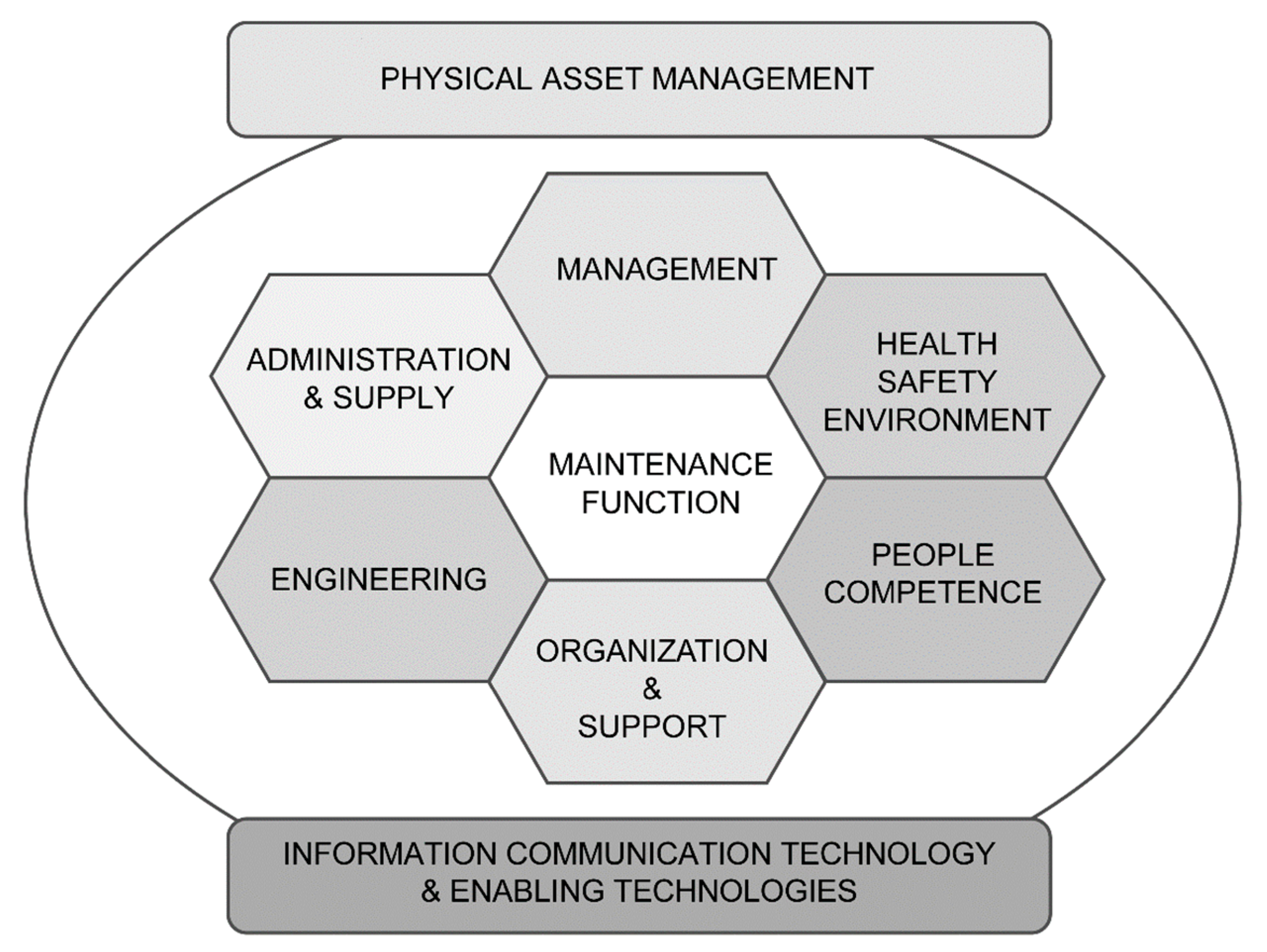
  • KPIs for “maintenance within physical asset management”;
  • KPIs for the sub-function of “maintenance management”;
  • KPIs for the sub-function of “maintenance engineering”;
  • KPIs for the sub-function of “organisation and support”;
  • KPIs for the sub-function “administration and supply”.
Neither the sub-functions “people competence” and “health-safety-environment (HSE)” nor the support function “information and communication technology” will be considered for the KPI formulation, as they are not directly related to the scope of the analysed scheduling framework.
The formulation and definition performance indicators for each sub-function are presented next. All indicators comparing different scenarios (or strategies) are used to compare a base scenario against a current scenario to be defined by the decision maker. In particular, for the opportunistic grouping strategy presented in [9], different scenarios (or strategies) are defined by the chosen tolerance.

2.3.1. KPIs for “Maintenance within Physical Asset Management”

The following indicators favour the optimal management of the life cycle of physical assets in order to achieve the established goals of the organisation in a sustainable way. Additionally, they highlight the importance of maintenance in the different stages of the life cycle and help maintenance management define long-term maintenance strategies.
Mean expected execution risk ( P A M 1 ) is defined as:
P A M 1 = i , j I , J i F i , j ( t s i , j ) N e
where N e : is the set of all activities, and i I .
Description: This KPI quantifies the mean failure probability for a given tolerance as the mean failure risk associated with the execution of all activities within the planning horizon.
Mean expected failure risk variation ( P A M 2 ) is defined as:
P A M 2 = P A M 1   ( current ) P A M 1   ( base )
Description: This KPI measures the variation of mean failure risk ( P A M 1 ) between the base scenario (i.e., 0% tolerance) and the current scenario (i.e., x% tolerance).

2.3.2. KPIs for Sub-Function “Maintenance Management”

The standard defines this sub-function as the combination of resources, disciplines, competences, and tools to define medium-term planning according to the industrial plan of the company. It is also encompasses coordination and control of activities implemented for physical assets to achieve the objectives within the existing framework and constraints.
Expected availability based on time ( M M 1 ) is defined as:
M M 1 = 1 T u T ,     w i t h
T u = i I j J i d i , j + i I j J i T i , j c ( t s i , j )
where T u : is the expected downtime due to preventive and corrective interventions, and d i , j is the downtime of the jth execution of activity i , where ( i , j ) I × J i .
Description: This KPI Measures the proportion of the horizon time ( T ) in which the system is expected to be available, considering scheduled and unscheduled (due to failure) stoppages ( T u ). The indicator considers the amount of time for unscheduled stoppages as the mean failure risk for the system ( P A M 1 ) multiplied by the mean duration of the corrective actions for all the activities. Perfect corrective maintenance is assumed for every expected failure.
Expected availability percentage variation ( M M 2 ) is defined as:
M M 2 = M M 1   ( current ) M M 1   ( base )
Description: This KPI measures the expected availability (MM1) variation between a base scenario and a current scenario.
Expected number of stoppages ( M M 3 ) is defined as:
M M 3 = | { k K : ρ k 0 } | + i I j J i 0 T λ i , j ( x )   d x
Description: This KPI indicates the number of scheduled and unscheduled (due to failure) stoppages for the current strategy. It assumes that the number of stoppages due to failure is equal the closest integer to the mean failure probability of the system.
Expected number of stoppages variation ( M M 4 ) is defined as:
M M 4 = M 3   ( curent ) M 3   ( base )
Description: This KPI measures the percentage variation in the expected number of stoppages between the current strategy and the base strategy

2.3.3. KPIs for Sub-Function “Maintenance Engineering”

Maintenance engineering is the discipline and process whereby competence, skills, tools, and techniques to support and develop maintenance activities are applied in a safe, sustainable, and cost-effective way throughout the life cycle.
Maintenance scheduling mean absolute deviation ( M E 1 ) is defined as:
M E 1 = i I j J i | t s i , j t e i , j | N e
where t s i , j is the actual start time for the jth execution of activity i , and t e i , j is the tentative execution time for the jth execution of activity i .
Description: This KPI measures the mean absolute deviation of the tentative execution times ( t e i , j ) of the activities regarding their actual execution time ( t s i , j ), e.g., if M E 1 = 0.5 , on average, the execution dates are 0.5 weeks away from their planned date, whether they are early or late.
Average utilisation of tolerance for advancement ( A A V ) is defined as:
A A V = i I j J i | t s i , j t e i , j | e × T i i J i | J i | t s i , j < t e i , j
where T i is the defined periodicity of activity i , and e is the percentage of the periodicity ( T i ), which is defined as tolerance for the current scenario.
Description: This KPI measures the average percentage proportion of the available tolerance ( e × T i ) employed to advance the execution time of the jth execution of activity i when moved forward, e.g., if the value of this indicator is 20%, on average, executions that are being advanced use only 20% of their available time window.
Average utilisation of tolerance for delay ( D A V ) is defined as:
D A V = i I j J i | t s i , j t e i , j | e × T i i J i | J i | t s i , j > t e i , j
Description: This KPI measures the average percentage proportion of the available tolerance ( e × T i ) employed to delay the execution time of the jth execution of activity i when delayed.
Preserved activities proportion ( f 0 ) is defined as:
f 0 = | I J 0 | i J i | J i | ,     I J 0 = { i , j :   t s i , j = t e i , j ,   ( i , j ) I × J i }
Description: This KPI informs the proportion of preserved activities (i.e., t s i , j = t e i , j ) regarding the total number of executions of all activities.
Preserved activities proportion ( f A ) is defined as:
f A = | I J | i J i | J i | ,     I J = { i , j :   t s i , j < t e i , j ,   ( i , j ) I × J i }
Description: This KPI informs the proportion of advanced activities (i.e., t s i , j < t e i , j ) regarding the total number of executions of all activities.
Preserved activities proportion ( f D ) is defined as:
f D = | I J + | i J i | J i | ,     I J + = { i , j :   t s i , j > t e i , j ,   ( i , j ) I × J i }
Description: This KPI informs the proportion of delayed activities (i.e., t s i , j > t e i , j ) regarding the total number of executions of all activities.

2.3.4. KPIs for Sub-Function “Organisation and Support”

This sub-function is a combination of resources for internal and external maintenance, such as people, spares, tools, equipment, information, methodologies, processes, standards, best practices, ICTs, etc., necessary to provide the required maintenance services, aiming for the best performance in terms of safety, productivity, effectiveness, quality, and service level.
Preventive workforce load ( O & S 1 ) is defined as:
O & S 1 = w k = i Ρ k r i ,     k K
where r i is the workforce required to perform activity i .
Description: This KPI measures the number of workers required for the execution of maintenance activities during any time window in which no activities are starting or finishing. It is highly recommended for this indicator to be analysed over a workload balance plot.
Mean workforce load ( O & S 2 ) is defined as:
O & S 2 = k K w k
Description: This KPI measures the average number of workers required for preventive maintenance activities over the time horizon ( T ) for the strategies associated with x % tolerance.

2.3.5. KPIs for Sub-Function “Administration and Supply”

This sub-function mainly addresses the following three areas: (1) compliance of all economic practices and procedures of maintenance; (2) accounting activities and suitable procedures for all maintenance, as well as budget and cost control; and (3) supply chain management to purchase and provide all the required technical support.
Relative strategy cost ( A & S 1 ) is defined as:
A & S 1 = S C x % S S x %
where:
S C = i I j J i ( c u l i × u l i , j ) + i I j J i ( c c i × 0 T λ i , j ( x )   d x ) + u w × ( M M 1 ( b a s e ) M M 1 ( c u r r e n t ) ) × T
S S = ( | { k K : ρ k 0 } | ( b a s e ) | { k K : ρ k 0 } | ( c u r r e n t ) ) × c s + u w × ( M M 1 ( c u r r e n t ) M M 1 ( b a s e ) ) × T
c u l i : is the cost of the useful life of activity i .
u l i , j : is the amount of useful life wasted due to the advance of the jth execution of activity i .
c c i : is the cost associated with a corrective intervention of activity i .
u w : is the cost (or saving) of the system to operate without stoppages in one week.
c s : is the setup cost.
Description: This KPI measures the ratio between strategy costs ( S C ) and strategy savings ( S S ), showing the proportion of the strategy savings that is imputable to the strategy costs, i.e., how much of the savings due to the strategy are lost due to additional costs incurred due to the implementation of the strategy. S C is calculated simply the sum of the wasted useful lifetime plus the corrective intervention cost multiplied by the number of failures plus the inefficiency cost as the cost due to the difference between availability in the current scenario and the base scenario. Finally, S S is calculated as the sum of the setup cost multiplied by the number of stoppages plus the inefficiency savings. As an example, if a current strategy presents A S 1 = 15 % , the cost of the current strategy represents only 15% of the total savings achieved by the current strategy.
Timely inefficiency deviation ( A & S 2 ) is defined as:
A & S 2 = U x % U 0 % U 0 % ,
U = T u T
Description: This KPI indicates the percentage deviation of inefficiency measured as the percentage difference of unavailability between strategies. It is assumed that inefficiency cost is proportional to the unavailability of the system.
Mean Time Between Orders ( A & S 3 ) is defined as:
Before presenting a definition for this indicator, it is necessary to define a set containing all moments in which an order is issued. It is assumed that orders are issued whenever a total quantity of “ m ” spare parts have been employed. Furthermore, it is also assumed that, without losing generality, the use of spare parts is equal to the number of workers required for each activity. Hence, set T c is defined as follows:
T c = { t n [ 0 , T ] : k K w k m = n ,     n , m }
Therefore, the mean time between orders is:
A & S 3 = n = 1 | T c | 1 ( t n t n + 1 ) | T c |
Description: This KPI measures the mean time between the moments where a spare-parts purchase order is issued, assuming they are issued at the same time that “ m ” amount of the resource has been consumed, where “ m ” is a parameter that can be set by the decision maker. For illustrative purposes only, this parameter is set to 25, which means that only 25 workers are available in the plant.

2.4. Instance Definition

The base scenario in which to develop the algorithm and measure the associated indicators is described next.
In this research, we employ a system wherein a set of preventive maintenance activities is defined, of which 6 activities must be performed under a certain periodicity for each one of them over a time horizon T = 26 weeks. These activities are scheduled and grouped (if feasible) by the algorithm considering the use of time tolerance for each execution. Perfect maintenance is assumed for all executions, and non-negligible duration is assumed for the preventive maintenance activities.
The parameters for the instance used in this article are as follows:
The values for periodicity and maintenance task duration for each activity are listed in Table 1; these parameters are the same as in [7]. Furthermore, the parameters for the Weibull distribution of each activity are shown in Table 2 and were set considering a high shape parameter to simulate a high failure rate at late times and scale parameter equal to five times the periodicity of the preventive maintenance to ensure high levels of reliability between interventions. These parameters are selected with the aim of reducing focus on corrective maintenance, instead focusing on the performance of the grouping strategy.
The system parameters for setup cost ( c s ) and inefficiency cost ( u w ) are presented in Table 3. These values were chosen to depict the behaviour of the indicators related to cost and should be further studied to improve the accuracy of the report.
Finally, the parameters assumed for the calculation of the indicators defined above are presented in Table 4.
These values are selected considering that:
  • The mean time for a corrective maintenance intervention ( c m t i ) is 10% of the periodicity of the activity;
  • The workforce needed for an activity (ri) is 10 times the duration of the activity;
  • The cost of the unemployed useful life of the asset (culi) and cost of corrective intervention (cci) are set to 100 and 1000, respectively, for all activities.

2.5. Report Design

As mentioned, Power BI is the reporting tool employed in this article, wherein it is possible to natively integrate Python scripts as a data source. The report evaluates 10 different scenarios (or tolerances), from 0% (no grouping) through 10%, with increases of 1%. After the data source has been defined in Power BI, it is presented in the form of several plots and graphics for easy understanding and decision making. The latter is most important, and therefore, the design of the report is conceived to guide the decision maker through the indicators, first addressing a general overview of the different strategies, followed by sections corresponding to each of the maintenance functions. The sections presented to the decision maker are as follows:
  • Overview: This section is divided into a left side and a right side. Both sides show the main indicators for the decision maker. On the left side, it is possible to observe the behaviour of availability, number of stoppages, mean failure risk and, inefficiency cost for any chosen tolerance. On the right side, it is possible to observe the variation of the left-side indicators, considering the difference between a 0% tolerance scenario and a chosen scenario.
  • Best Performing Strategies: This section shows the strategies that perform best with respect to availability, number of stoppages, and failure risk.
  • Activity Risk Assessment: This section shows the mean failure risk for each activity and tolerance.
  • Physical Asset Management: This section shows the variation of the mean failure risk regarding the 0% strategy.
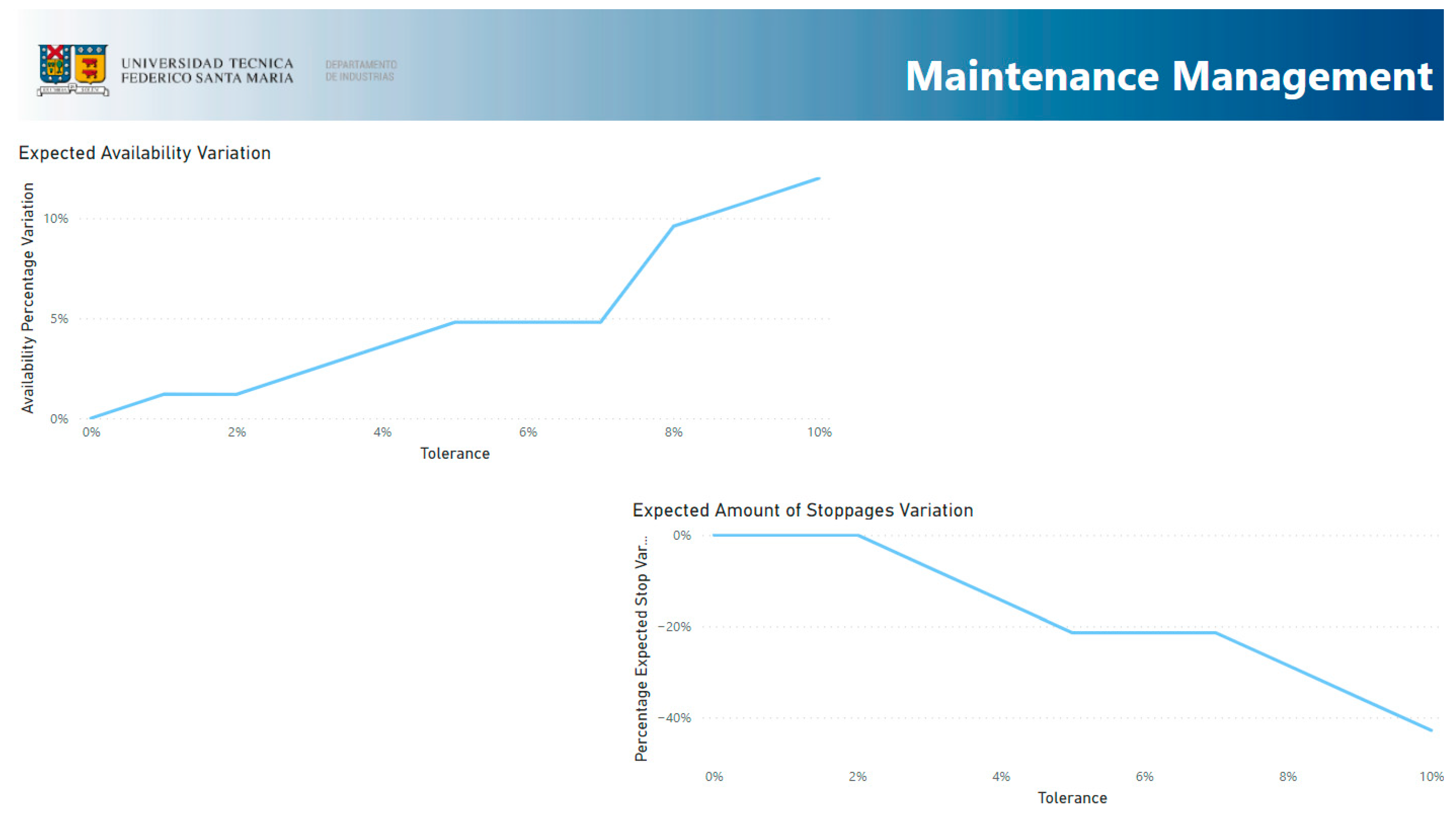
  • Maintenance Management: This section shows the availability variation and stoppage variation regarding the 0% strategy.
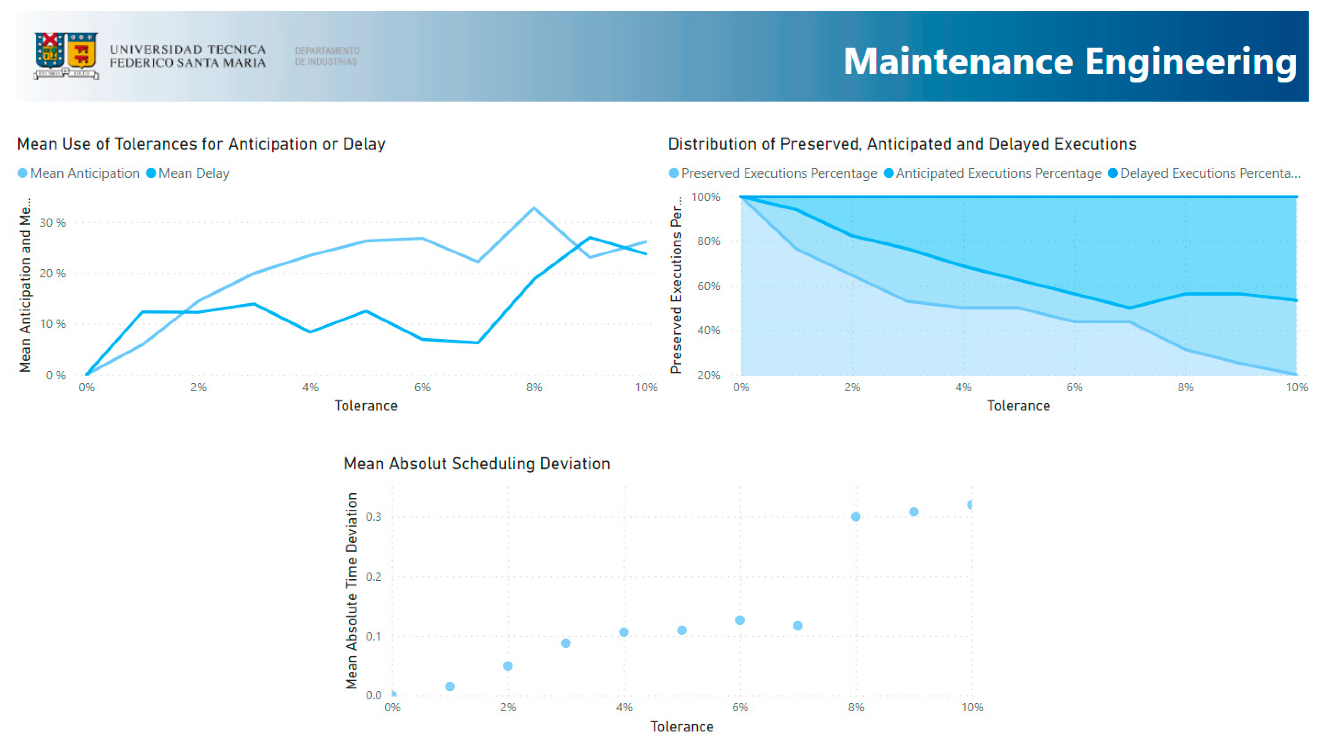
  • Maintenance Engineering: This section presents the legacy indicators from the original algorithm and the deviation of the scheduling regarding the 0% strategy.
  • Organisation and Support: This section presents a workforce balance of all time horizons, allowing the decision maker to choose and compare between tolerances with respect how human resources are employed. It also presents the mean workforce load for the chosen tolerance.
  • Administration and Supply: The final section presents the inefficiency deviation, relative strategy cost, and the mean time between orders for each strategy.

3. Results and Discussion

In general terms, a reporting tool was developed to highlight the most influential indictors for maintenance management. The sequence for the report is aimed to support fast and accurate strategic decision making in the beginning, continuing with the presentation of more specific indicators for the maintenance function. This perspective improves the accuracy of decisions by first presenting the most critical indicators aligned with the vision and objectives of the organisation in order to support information when strategic decisions are made. Furthermore, the second part of the report presents information about specific maintenance functions to support tactical and operational decisions related to how well the strategic decisions and objectives are being achieved when performing maintenance activities. To summarize, the first two sections of the report relate to strategic decisions regarding “which tolerance” to choose, and the remaining six sections relate to the performance of each maintenance function under a specific strategy in order to control and improve it.

3.1. Overview

As mentioned, in the Overview section (see Figure 2), the main indicators for a chosen strategy (0% in this case) are presented, with their variation on the right side of the display (7% for this case). In the 0% tolerance scenario, scheduling presents 64.10% availability, with 14 stoppages, an average of 3.74% failure risk, and an inefficiency cost of USD 9330. From the base scenario (0%) to the 7% scenario, there is an increase in availability and, as well as a decrease in the mean failure risk, number of stoppages, and inefficiency deviation. This suggests that the objective of the algorithm of minimizing the number of stoppages directly impacts on the availability of the system, although it is not clear whether there is a relationship between failure risk and the number of stoppages. The latter is supported by how many (proportionally) activities have been advanced, preserved, or delayed. When 50% of the activities have been delayed with no significant impact on the mean risk, it can be concluded that there is no relationship between the risk and the number of stoppages.

3.2. Best-Performing Strategies

This section presents (see Figure 3), in a simple way, the strategies that achieve the best performance regarding the expected availability, number of stoppages, and mean failure risk. It is possible to observe that for availability and stoppages, the strategy that best performs for both cases is the 10% scenario. This is consistent with the main objective of the algorithm, which is to minimise the number of scheduled stoppages to directly increase availability. On the contrary, given that the algorithm has no regard for the risk assumed, the lowest risk is achieved in the 6% tolerance scenario, suggesting that this strategy may favour the advancement of more activities or the delay of activities with low risk. This confirms that through assertive scheduling using tolerances, it is possible to decrease risk while achieving increased availability.

3.3. Activity Risk Assessment

In this section (see Figure 4), the mean risk for each activity is presented; activities associated with the lowest risk are also the activities with lowest periodicity. This suggests that periodicity is directly related to risk and that it might be advisable to avoid delaying these activities as much as possible. Moreover, with around 8% tolerance, it is possible to observe an increase on the mean risk for activity 5, which is one of the activities with highest base risk; this is consistent with the fact that 8% and 9% are the strategies with the highest risk.

3.4. Physical Asset Management

Regarding the behaviour of the mean failure risk presented in Figure 5, this section confirms two aspects. First, it confirms that the algorithm has no regard for risk, showing an unclear behaviour or tendency towards minimising risk, which is the reason behind the difference of risk between the 7% and 8% scenarios, wherein there is an important increase in risk (8% tolerance) resulting from an initial decrease in risk (7% tolerance). Second, it confirms the impact on risk of the activities with higher periodicities, showing an important variation of almost 5% of failure risk for the strategy with 9% tolerance.

3.5. Maintenance Management

This section (see Figure 6) supports the conclusion regarding the inverse relationship between availability and stoppage variation, showing that fewer stoppages lead to a more available system. In fact, both curves have almost an identical inverse tendency.

3.6. Maintenance Engineering

Regarding maintenance engineering presented in Figure 7, the behaviour of the mean use of tolerance shows a tendency towards anticipation, meaning that when the algorithm choses to anticipate an execution, it tends to make an exhaustive use of its range. On the other hand, considering the proportion of advanced, delayed, and preserved activities, a tendency towards delaying activities is observed. These two behaviours (the use of tolerance towards anticipation and the high proportion of delayed activities) seem to be in opposition at first, but further analysis reveals that despite more activities being delayed for higher-tolerance strategies, the use of tolerance for delayed activities is not exhaustive. On the contrary, such low proportions for advanced activities tend to result in an aggressive use of tolerance.

3.7. Organisation and Support

This section presents an overview regarding the workforce load of the preventive maintenance activities. The balance for the 9% strategy is presented in Figure 8, assuming a total of 25 available workers for the executions. Considering the latter, there is a peak of workforce load between the 22nd and 24th week, which may suggest that the strategy associated with 9% tolerance is unfeasible or that the decision maker should prepare for a higher workload on a specific date.
Moreover, this view enables not only the planning of workforce load but also planning for the use of different resources within the system.

3.8. Administration and Supply

Regarding administrative indicators presented in Figure 9, they exhibit a tendency towards a more efficient process. Inefficiency deviation confirms that there is a proportional relationship between grouping and the improvement of inefficiencies, meaning that whenever groups are formed, more time is available for production. Furthermore, regarding the cost associated with each strategy, it is possible to observe that for every strategy, the additional cost is no more than 15% of the savings for the same strategy; this is mainly explained by the high setup cost of the system, meaning that whenever groupings are made, the savings of the setup cost are considerably higher than the additional costs incurred due to grouping. Moreover, the mean time between orders decreases around 5% tolerance, meaning that because of grouping, there is a more intense use of resources, and thus, spare-parts orders must be issued more frequently.
Despite the analysis, the results of performance are not focused on the maintenance sub-functions they contribute to the overall analysis of the impact and differences between the possible grouping strategies.
One of the goals of preventive maintenance is to avoid the consequences of failures, especially those related to high cost or hazards. The developed reporting tool addresses this issue by proposing a specific perspective and methodology for the calculation of risk. Furthermore, the flexibility of the tool also allows the script to be modified in order to support other risk modelling methodologies. Therefore, the accuracy of the measuring methodology and risk assessment flexibility ensure that the strategies are evaluated with a strict focus on preventive maintenance.

4. Conclusions

Aligned with the main objective of this article and its scope, a reporting tool was successfully developed to address timely decisions and easy interpretation, enabling decision makers to quickly decide between strategies and accurately analyse different scenarios. Furthermore, the designed tool is able to adapt to different algorithms, as it requires little information from the process, enabling future work or even implementation in a real system or case study. The latter is a major improvement for maintenance management and grouping strategies in particular, as the same tool is able to measure different scheduling approaches with little information needed, improving decision quality and the capacity to compare different strategies from varied sources.
The developed indicators obtained through a rigorous analysis of the algorithm and the maintenance standards enable a transversal and disaggregated view of the different areas directly or indirectly related to the maintenance function, leading to the possibility of deciding not only which tolerance is best-suited for a given system but to manage different aspects of maintenance before and after a tolerance has been chosen. In other words, is possible to decide which strategy to implement in parallel with other management decisions, such as how to manage the workforce, resources, and purchases.
To develop the indicators, it was necessary to perform a comprehensive analysis of the strength and weaknesses of the algorithm; based on this analysis, we determined that little and inaccurate information was available, resulting in a timeline perspective enabling precise measurement of all developed indicators. This suggests that further improvements can be achieved by considering this perspective in relation to future algorithms or modifications of the original algorithm. The precision achieved in this study improves the information available for decision makers, also improving the quality of decisions. Moreover, the developed perspective may even be used as a baseline to develop new grouping algorithms addressing more precise decisions not only based on time but also risk and resource allocation.
Despite the limitations of Power BI, it was possible to design and implement a simple and efficient report that precisely measures each of the designed indicators, presenting them in an easy-to-use format. Moreover, it was possible to grant autonomy to the report, enabling the decision maker to adjust, modify, or even completely change the studied instance and parameters.
Whenever changes are made to the parameters of the algorithm, important changes can be observed in the algorithm, accounting for the precision of the same and the variability associated with implementing different scenarios. Considering that only one scenario was presented, there is an opportunity to test more instances for the same algorithm to define and analyse tendencies and behaviour. Additionally, it is even possible to test different algorithms under the same report, enabling comparisons of possible decisions in order to determine which algorithm is best-suited for each case.
Regarding risk analysis of the strategies, it is necessary to integrate a risk variability analysis, mainly because whenever tolerance is available, there is a range of possible risks to assume related to how much of the tolerance is being used for each execution and activity. In other words, a specific tolerance hides a wide range of possibilities that are not measured in this article.
The analysed algorithm tends to disregard risk but is possibly compensated by the advancement of other tasks and the savings achieved due to lower setup costs in contexts wherein the setup cost is high. As a recommendation, the algorithm must address failure risk when grouping; it is not enough to address availability though a minimal number of stoppages because there is no certainty that the algorithm will propose high-availability scenarios with even higher risk, meaning that even if the strategy seems promising, it may implicate high corrective costs or even hazardous risks. Considering risk, incorporating availability and resource availability into the algorithm may considerably improve its accuracy and feasibility to be implemented in a real-world case, resulting in more efficient and leaner processes.
Finally, regarding the scalability of the report, it is limited in relation to the computational capacity available to process the algorithm, which may be overcome by new technologies, such as machine learning, which is already embedded and ready to use in Power BI, enabling future work making use of such tools.

Author Contributions

Conceptualization, P.V., N.C.P. and R.M.; data curation, N.C.P.; formal analysis, P.V. and R.M.; investigation, N.C.P. and P.V.; methodology, N.C.P., R.M. and F.K.; project administration, P.V. and F.K. All authors have read and agreed to the published version of the manuscript.

Funding

This research received no external funding.

Institutional Review Board Statement

Not applicable.

Informed Consent Statement

Not applicable.

Data Availability Statement

Not applicable.

Conflicts of Interest

The authors declare no conflict of interest.

References

  1. de Jonge, B.; Scarf, P.A. A Review on Maintenance Optimization. Eur. J. Oper. Res. 2020, 285, 805–824. [Google Scholar] [CrossRef]
  2. Kristjanpoller, F.; Cárdenas-Pantoja, N.; Viveros, P.; Mena, R. Criticality Analysis Based on Reliability and Failure Propagation Effect for a Complex Wastewater Treatment Plant. Appl. Sci. 2021, 11, 10836. [Google Scholar] [CrossRef]
  3. Kristjanpoller, F.; Viveros, P.; Cárdenas, N.; Pascual, R. Assessing the Impact of Virtual Standby Systems in Failure Propagation for Complex Wastewater Treatment Processes. Complexity 2021, 2021, 9567524. [Google Scholar] [CrossRef]
  4. Pandey, M.; Zuo, M.J.; Moghaddass, R. Selective Maintenance Scheduling over a Finite Planning Horizon. Proc. Inst. Mech. Eng. Part O J. Risk Reliab. 2016, 230, 162–177. [Google Scholar] [CrossRef]
  5. Do, P.; Barros, A. Maintenance Grouping Models for Multicomponent Systems. In Mathematics Applied to Engineering; Elsevier: London, UK, 2017; pp. 147–170. [Google Scholar]
  6. Ding, S.-H.; Kamaruddin, S. Maintenance Policy Optimization—Literature Review and Directions. Int. J. Adv. Manuf. Technol. 2014, 76, 1263–1283. [Google Scholar] [CrossRef]
  7. Viveros, P.; Mena, R.; Zio, E.; Campos, S. Optimal Grouping and Scheduling of Preventive Maintenance Activities. In Proceedings of the 30th European Safety and Reliability Conference and the 15th Probabilistic Safety Assessment and Management Conference, Venice, Italy, 1–5 November 2020; Baraldi, P., Di Maio, F., Zio, E., Eds.; Research Publishing Services: Venice, Italy, 2020; pp. 2915–2922. [Google Scholar]
  8. Mena, R.; Viveros, P.; Zio, E.; Campos, S. An Optimization Framework for Opportunistic Planning of Preventive Maintenance Activities. Reliab. Eng. Syst. Saf. 2021, 215, 107801. [Google Scholar] [CrossRef]
  9. Viveros, P.; Mena, R.; Zio, E.; Miqueles, L.; Kristjanpoller, F. Integrated Planning Framework for Preventive Maintenance Grouping: A Case Study for a Conveyor System in the Chilean Mining Industry. Proc. Inst. Mech. Eng. Part O J. Risk Reliab. 2021, 1748006X2110537. [Google Scholar] [CrossRef]
  10. Wu, S. Preventive Maintenance Models: A Review. In Replacement Models with Minimal Repair; Springer: London, UK, 2011; Volume 43, pp. 129–140. [Google Scholar]
  11. Blanchard, B.S.; Blyler, J.E. System Engineering Management; John Wiley & Sons, Inc.: Hoboken, NJ, USA, 2016; ISBN 9781119178798. [Google Scholar]
  12. Tarelko, W. Control Model of Maintainability Level. Reliab. Eng. Syst. Saf. 1995, 47, 85–91. [Google Scholar] [CrossRef]
  13. Al-Turki, U.M. Maintenance Planning and Scheduling. In Handbook of Maintenance Management and Engineering; Springer: London, UK, 2009; pp. 237–262. [Google Scholar]
  14. Nicolai, R.P.; Dekker, R. Optimal Maintenance of Multi-Component Systems: A Review. In Complex System Maintenance Handbook; Springer: London, UK, 2008; Volume 8, pp. 263–286. [Google Scholar]
  15. Tsang, A.H.C. Strategic Dimensions of Maintenance Management. J. Qual. Maint. Eng. 2002, 8, 7–39. [Google Scholar] [CrossRef]
  16. Kumar, U.; Galar, D.; Parida, A.; Stenström, C.; Berges, L. Maintenance Performance Metrics: A State-of-the-Art Review. J. Qual. Maint. Eng. 2013, 19, 233–277. [Google Scholar] [CrossRef] [Green Version]
  17. Parida, A.; Kumar, U.; Galar, D.; Stenström, C. Performance Measurement and Management for Maintenance: A Literature Review. J. Qual. Maint. Eng. 2015, 21, 2–33. [Google Scholar] [CrossRef]
  18. Eckerson, W.W. Performance Dashboards; Eckerson, W.W., Ed.; Wiley: Hoboken, NJ, USA, 2012; ISBN 9780470589830. [Google Scholar]
  19. Shohet, I.M. Key Performance Indicators for Strategic Healthcare Facilities Maintenance. J. Constr. Eng. Manag. 2006, 132, 345–352. [Google Scholar] [CrossRef]
  20. Wireman, T. Developing Performance Indicators for Managing Maintenance; Industrial Press: New York, NY, USA, 2005; ISBN 0831131845. [Google Scholar]
  21. Lynch, R.L.; Cross, K.F. Measure Up-The Essential Guide to Measuring; Mandarin: London, UK, 1991. [Google Scholar]
  22. Parida, A. Study and Analysis of Maintenance Performance Indicators (MPIs) for LKAB: A Case Study. J. Qual. Maint. Eng. 2007, 13, 325–337. [Google Scholar] [CrossRef] [Green Version]
  23. Anggradewi, P.; Aurelia; Sardjananto, S.; Ekawati, A.D. Improving Quality in Service Management through Critical Key Performance Indicators in Maintenance Process: A Systematic Literature Review. Qual.-Access Success 2019, 20, 72–79. [Google Scholar]
  24. Stefanovic, M.; Nestic, S.; Djordjevic, A.; Djurovic, D.; Macuzic, I.; Tadic, D.; Gacic, M. An Assessment of Maintenance Performance Indicators Using the Fuzzy Sets Approach and Genetic Algorithms. SAGE J. 2015, 231, 15–27. [Google Scholar] [CrossRef]
  25. Microsoft What Is Power BI?—Power BI|Microsoft Docs. Available online: https://docs.microsoft.com/en-us/power-bi/fundamentals/power-bi-overview%0Ahttps://docs.microsoft.com/en-us/power-bi/fundamentals/power-bi-overview%0Ahttps://docs.microsoft.com/fi-fi/power-bi/fundamentals/power-bi-overview (accessed on 9 November 2021).
  26. BS-EN 15341:2019; Maintenance—Maintenance Key Performance Indicators. British Standard Institute: British, UK, 2019; ISBN 978 0 580 97964 4.
  27. UNE-EN 17007:2018; Maintenance Process and Associated Indicators. Asociación Española de Normalización (UNE): Madrid, Spain, 2017.
Figure 1. Maintenance functions and core framework (source: CEN [26]).
Applsci 12 05386 g001
Figure 2. Overview section.
Applsci 12 05386 g002
Figure 3. Best-performing strategies section.
Applsci 12 05386 g003
Figure 4. Activity risk assessment section.
Applsci 12 05386 g004
Figure 5. Physical asset management section.
Applsci 12 05386 g005
Figure 6. Maintenance management section.
Applsci 12 05386 g006
Figure 7. Maintenance engineering.
Applsci 12 05386 g007
Figure 8. Organisation and support section.
Applsci 12 05386 g008
Figure 9. Administration and supply section.
Applsci 12 05386 g009
Table 1. Instance parameters.
Activity   ( i ) Periodicity   ( T i ) Duration   ( p i )
130.2
251
370.5
4111.5
5131.1
6171.3
Table 2. Weibull parameters.
Activity   ( i ) Shape   ( β i ) Location   ( γ i , j ) Scale   ( η i )
12015
22025
32035
42055
52065
62085
Table 3. System parameters.
c s u w
5001000
Table 4. Report parameters.
Activity   ( i ) c m t i r i c u l i c c i
10.321001000
20.5101001000
30.751001000
41.1151001000
51.3111001000
61.7131001000
Publisher’s Note: MDPI stays neutral with regard to jurisdictional claims in published maps and institutional affiliations.

