Article

Harmonic Extrapolation of Seismic Reflectivity Spectrum for Resolution Enhancement: An Insight from Inas Field, Offshore Malay Basin

by
Basil Onyekayahweh Nwafor
and
Maman Hermana
*
Centre for Subsurface Seismic Imaging, Institute of Hydrocarbon Recovery, Universiti Teknologi PETRONAS, Seri Iskandar 32610, Malaysia
*
Author to whom correspondence should be addressed.
Appl. Sci. 2022, 12(11), 5453; https://doi.org/10.3390/app12115453
Submission received: 8 April 2022 / Revised: 2 May 2022 / Accepted: 24 May 2022 / Published: 27 May 2022

Abstract

:

Featured Application

The workflow and the results presented in this article can be applied to post-processed and pre-processed seismic data to increase accuracy in the quality and interpretability of the data, as well as save cost and time for hydrocarbon exploration.

Abstract

For decades, how to improve the resolution limit of seismic data has been a concern for seismologists. For this reason, several geoscientists have proposed various methods of improving the bandwidth of the data. Discovering an easy and scientifically reliable means of improving seismic data resolution would undoubtedly help geophysicists interpret more complex details of the subsurface geology. In this study, we transformed the bandlimited time-domain seismic data to the frequency domain using the Fourier analysis method, and a basis pursuit atomic algorithm was applied to decompose the real and imaginary parts of the spectrum into summations of cosines and sines. The resultant reflectivity spectrum (in the frequency domain) was deconvolved by a pre-estimated wavelet spectrum to obtain the true earth’s reflectivity data spectrum and was subsequently extrapolated to beyond the original band limit. The result shows an extended bandwidth from 68 Hz to 161 Hz and 80 Hz to 170 Hz for both synthetic trace model and the main seismic data, respectively. Consequently, this improved vertical resolution of sub-seismic geologic features, such as crevasse splay, levee, barrier bar complex, lagoon inlet channels, alluvial fans, and fluvial channels, and shows subtle facies variations in Inas field.

1. Introduction

Accurate interpretation of seismic reflection data is one major contributing factor to successful oil and gas exploration. The success of a seismic geomorphology study is dependent not only on knowledge of sedimentological or stratigraphical principles and the local geological setting, but also on the quality of the seismic geomorphological imaging [1]. Notwithstanding that many advanced technologies, sophisticated computers, and software have been used in data acquisition and processing, there are still many challenges associated with the interpretation of seismic data, one of which is the seismic resolution problem [2]. It is still difficult to uncover the geologic stories recorded in seismic data volumes, especially when they are sub-seismic [3]. Seismic signal-to-noise ratio typically degrades with depth, and interpretation is hampered further at depth if the unit of interest is thin and well below seismic resolution. Furthermore, reflections from multiple thin beds commonly interfere with one another and form merged events, making object- or volume-based imaging more difficult [4]. To improve our understanding of hydrocarbon reservoirs, there is a need to enhance the resolution quality of the seismic data. Resolution is the ability to separate two features that are close together [5,6]. Because of the limited seismic bandwidth, there is a thickness below which seismic loops cannot be effectively distinguished [7]. Improving the bandwidth of seismic data has always been one of the primary concerns for geophysicists for decades because this would enable seismologists to interpret finer details of the subsurface geology, such as the extraction of stratigraphic, structural, and geomorphological details from seismic data; this has become indispensable because of the emerging complexities in the delineation, characterization, and development of hydrocarbon reservoirs [8].
There is a thickness below which seismic loops essentially have constant separation as a function of frequency bandwidth [9]. This thickness is known as the tuning thickness. The below-tuning effects are a result of the interference of wavelets, which are a function of geology as it changes vertically and laterally [10]. According to [2,8,11], the tuning thickness is a quarter of a wavelength for vertical resolution and (z + λ/4)2 for horizontal resolution. As shown below, Figure 1 depicts the synthetic seismic response of a theoretical wedge model. A simple layer wedging out from right to left is shown in Figure 1a. It was made from sand’s top and bottom reflectivities, with opposite polarities separated by a variable distance. Figure 1b depicts how the extracted amplitude (red dotted line) fluctuates with the actual wedge thickness. The thickness at which the amplitude is maximum is the tuning thickness.
Some five decades ago, Widess proposed λ/8 as the resolution limit of seismic data, where λ is the predominant wavelength in the data [8]. As a result of the presence of noise and the consequent broadening of the wavelet resulting from the spherical divergence of the seismic wavefront during its subsurface propagation, this resolution is usually assumed to be λ/4. According to this theory, the wavelength is the yardstick for resolution, which in turn depends on velocity and frequency. Because velocity generally increases with depth, Widess’ only variable and major parameter for determining resolution is frequency. Based on this theory and other contributing factors, several techniques have been used by scientists to overcome the interpretation problems posed by the limited seismic data bandwidth. These include detuning of seismic amplitude [9], wedge modeling [8], improvement of signal-to-noise ratio [11], enhancing the shape of wavelets for an improved bandwidth [12,13], spectral inversion [2,14], inverse Q filtering [15], spectral bluing and color inversion [16], sparse layer reflectivity inversion [17], and so on.
Several techniques have been particularly employed to boost the spectrum of the seismic data by arbitrarily increasing the data frequency. The authors of [18] proposed the loop reconvolution technique, in which the SEG-Y data is oversampled to avoid aliasing, and a new sparse spike reflectivity series weighted by the interpolated amplitudes at all the maxima and minima locations is generated. Then, the resulting reflectivity series is convolved with a suitably analytical high-frequency wavelet that is randomly calculated. The optimum frequency band for that dataset is determined by visual preference, without any mathematical control, and filters off all unwanted frequencies. The problem with this technique is that the spike does not represent the true reflectivity of the data. This method produces output that is correlated with the original peaks and troughs, which can lead to a misleadingly high correlation to synthetic data if the original well tie is also good [19]. Although it brings out better continuity of events in the fault zone, the author of [20] further confirmed that this technique also suffers from the drawback of boosting some noise.
Another enhancement technique as described by [19] is phase acceleration, which uses the instantaneous frequency of original data as a fundamental frequency and increases the seismic frequency by increasing the rate of change of the instantaneous phase. According to complex trace analysis, the bandlimited seismic signal can be viewed as the real component of a complex number representation (called the analytic trace), which provides a definitive separation for amplitude of the trace envelope and local phase content [21]. This representation permits explicit calculation and modification of the instantaneous frequency, which is the first derivative of the instantaneous phase in the time domain. The analytical signal S(t), of which the seismogram s(t) is the real part, is given by Equation (1) below.
S(t) = s(t) + is⊥(t) = A(t)ei¥(t)
where ¥ ( t ) is the instantaneous phase, A(t) is the instantaneous amplitude, and s⊥(t) is the quadrature series (Hilbert transform) of the real seismic trace. The author of [22] demonstrated that the dominant frequency of the data is the instantaneous frequency at the peak of the envelope. As a result, by multiplying the phase term by any desired amount, the instantaneous frequency and dominant frequency of the original trace can be directly changed. Equation (1) can then be used to calculate the frequency extrapolated trace SE(t).
S E ( t ) = A ( t ) i = 1 k ( c o s   m i ¥ ( t ) )  
where mi can be varied to sum an arbitrary number of invented bands to the original data. The drawback of this method is that it randomly invents frequency by varying the mi which is an integer (0, 1, 2, 3, 4, 5, 6, 7, 8, 9) parameter, and this can alter the original seismic signals.
In addition to seismic resolution enhancement, spectral decomposition and coherency have been employed to image stratigraphic and structural details, respectively [23]. Layer thicknesses [24,25], stratigraphic geometries [26], direct hydrocarbon indicators [27,28,29,30], enhancement of seismic bandwidth [23], and depositional models [31] have all been determined using spectral decomposition. Furthermore, spectral decomposition divides the seismic signal into discrete frequency sub-bands or horizons [25]. This is accomplished by converting seismic data from the time domain to the frequency domain [32]. However, the limitedness of the seismic bandwidth limits the geologic details that can be seen using this technique.
In this study, we were able to improve the spectral bandwidth of seismic data from the Inas Field, offshore Malay Basin, by using simple harmonic extrapolation principles, which included a combination of spectral decomposition and seismic inversion fundamentals. The technique applies a sparsity constraint that is unbiased against layer thickness [33]. It thus produces inverted earth models containing reliably thinner layers than would a conventional spare-spike inversion [17]. The bandwidth extension algorithm is fully described and tested in [17] and theoretical aspects of the validity of bandwidth extension are discussed and demonstrated in [19]. This was used to improve the resolution limit of seismic data below the generally accepted tuning thickness, where seismic amplitude and frequency response are more sensitive to thin beds [34,35,36,37]. The resulting broadband seismic data was spectrally decomposed to reveal the geomorphic and geologic features contained in the analysis layer conspicuously hidden by the original bandlimited data. These revealed features aided the interpretation and inference of the paleo-geology of the study area.

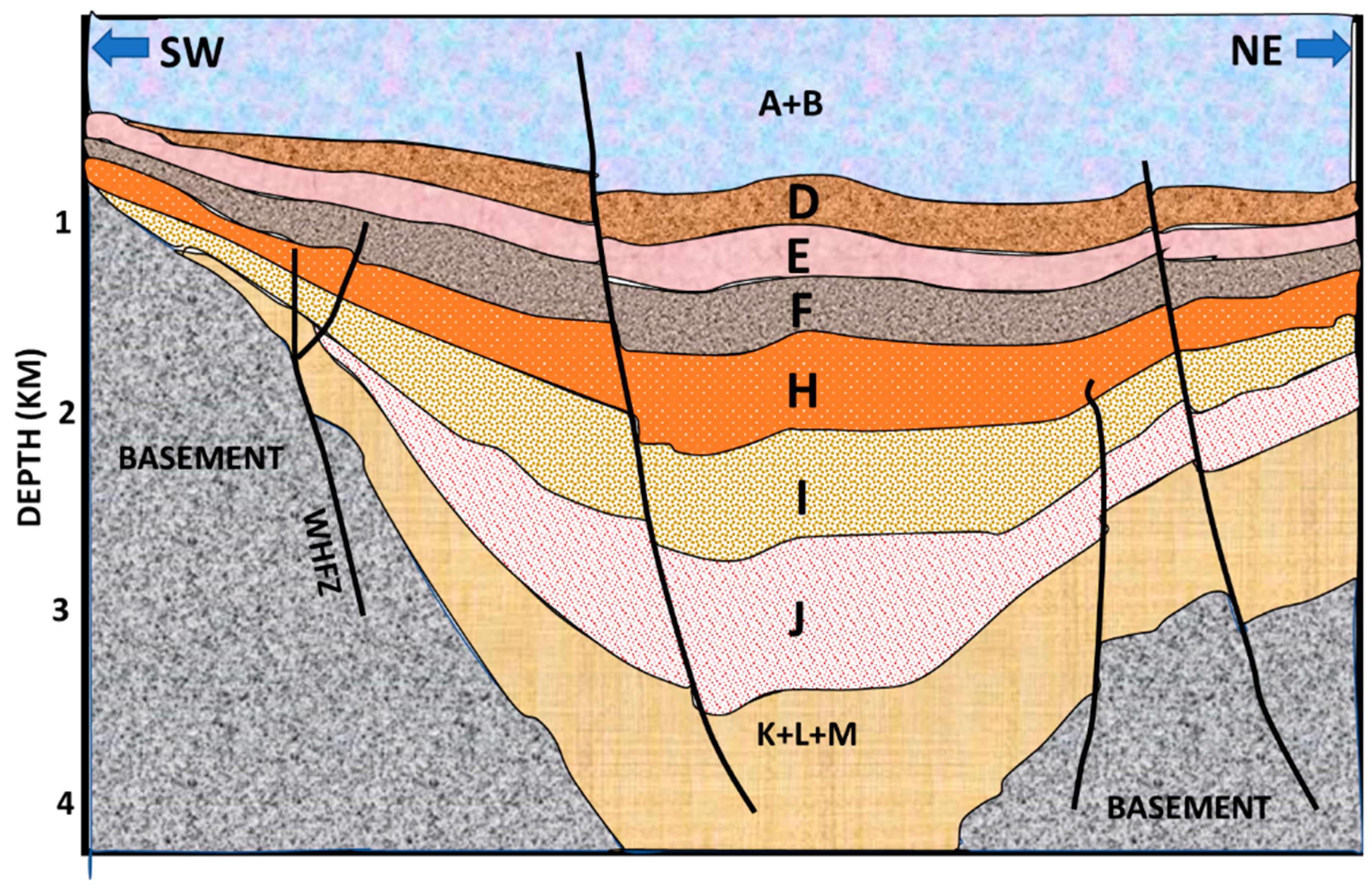
Brief Geologic Background of the Study Area

Inas Field is in the offshore Malay Basin, as indicated in Figure 2. It is an asymmetrical east–west compressional anticline with a moderate four-way dip closure that runs parallel to a significant north–south normal fault. The Malay Basin is organized into chronostratigraphic units, which are separated by regional reflectors that mark sequence borders or unconformities. The tectonic evolution of the basin is strongly linked to these sequence stratigraphic units, which were split into Groups A through M. The seismic data covered the entire stratigraphic intervals, starting from the basement to the recent deposits.
Post-depositional compressional deformation resulted in the creation of anticlinal structures and faults in the Inas Field, which contain hydrocarbons. The tectonic evolution of the Basin is closely linked to the sequence stratigraphic units [39]. The syn-rift evolution period reflects the extensional phase of basin development, when faulting controlled sedimentation and half grabens served as key depocenters, including consecutive sand and shale facies intercalations, mostly fluviolacustrine and alluvial deposits. After the Oligocene extensional faulting stopped around the time Groups L to D were deposited, the tectonic or thermal phase began. The presence of shale successive coal strata indicates that the shoreline was close to the coast at the time. During this time, there was a cyclic succession of marine, tidal estuary, coastal, and fluvial deposits. The progradational stacking of lacustrine channels and bounded erosional surfaces deposited Groups E and D as shown in Figure 3. Around the late Miocene to Quaternary epoch, the final subsidence phase was deposited. It was a time when there was little tectonic activity and only minor subsidence owing to thermal cooling. Due to the low energy of the mostly shallow marine environment, there was a full open marine transgression at this time, resulting in the deposition of Groups A and B, which mainly consisted of shale and silt.

2. Materials and Methods

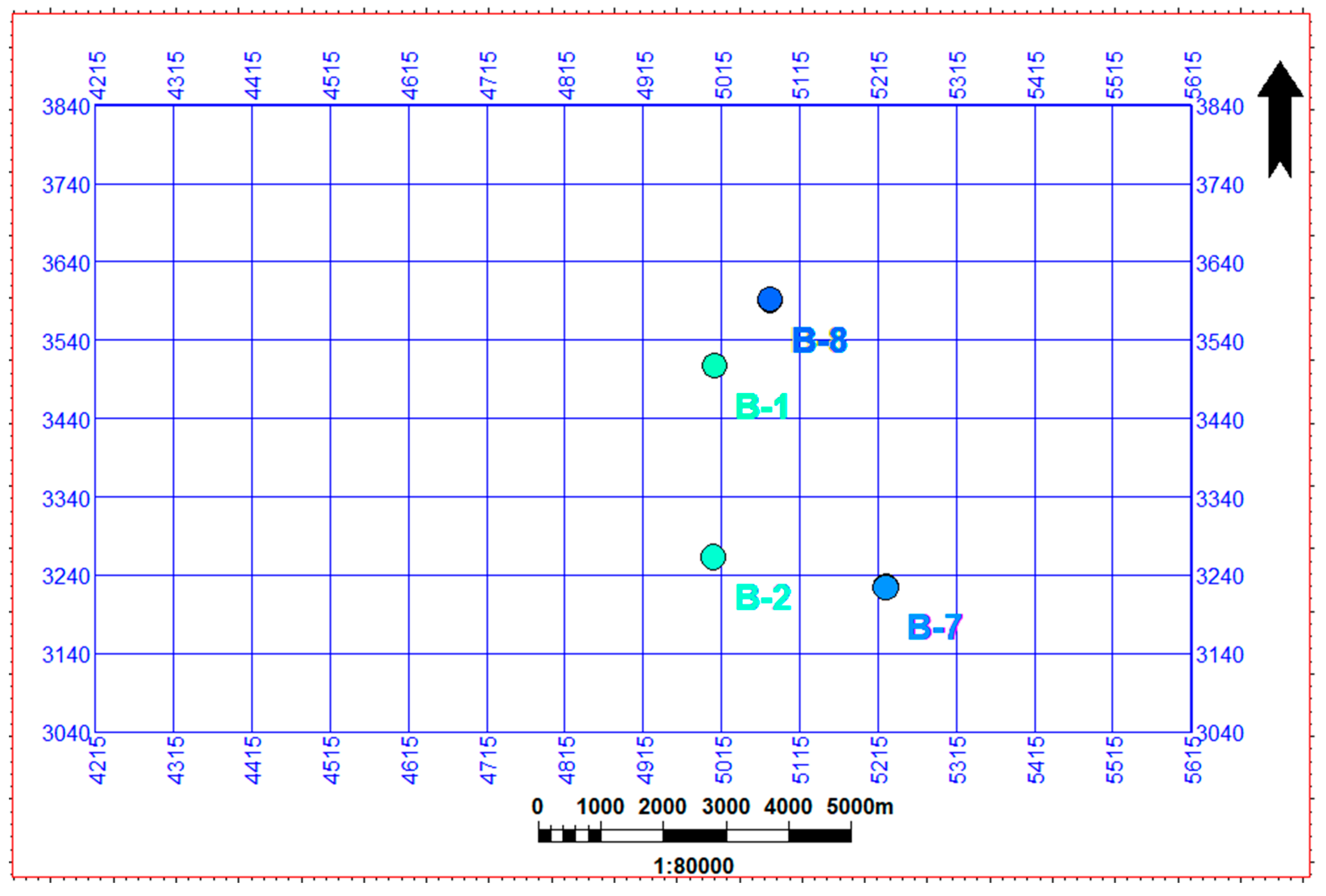
2.1. Data Presentation

Seismic data: post-stack time migrated full-stack seismic data with an angle range of 5–40 degrees were used in this study. The seismic data have a dominant frequency of 30 Hz at the reservoir interval and a bandwidth of 80 Hz. Its sample interval is 2 ms with an approximate tuning thickness of 32 m at the reservoir interval. Figure 4 shows the base map of the seismic data, with a dip line range of 3040 to 3840 and strike line range of 4215 to 5615.
Well logs: Eight wells were drilled in the field, but only four out of them have the required log suites for this analysis. These wells are B-1, B-2, B-7, and B-8 (Figure 4). All the required composite logs, such as compressional sonic, shear sonic, density, gamma-ray, etc., were available and adequately covered the interval of interest. The check shot data, the vertical seismic profiling data, and interval velocity data were provided and carefully integrated to perform a robust well–seismic tie. The seismic–well tie process was used to validate the accuracy of the input wavelet.
Seismic wavelets: This technique requires an intensive wavelet analysis. First, we used an analytical wavelet for the initial analysis, followed by a statistical wavelet from seismic data, and finally, a deterministic wavelet was extracted by combining the well and the seismic data.

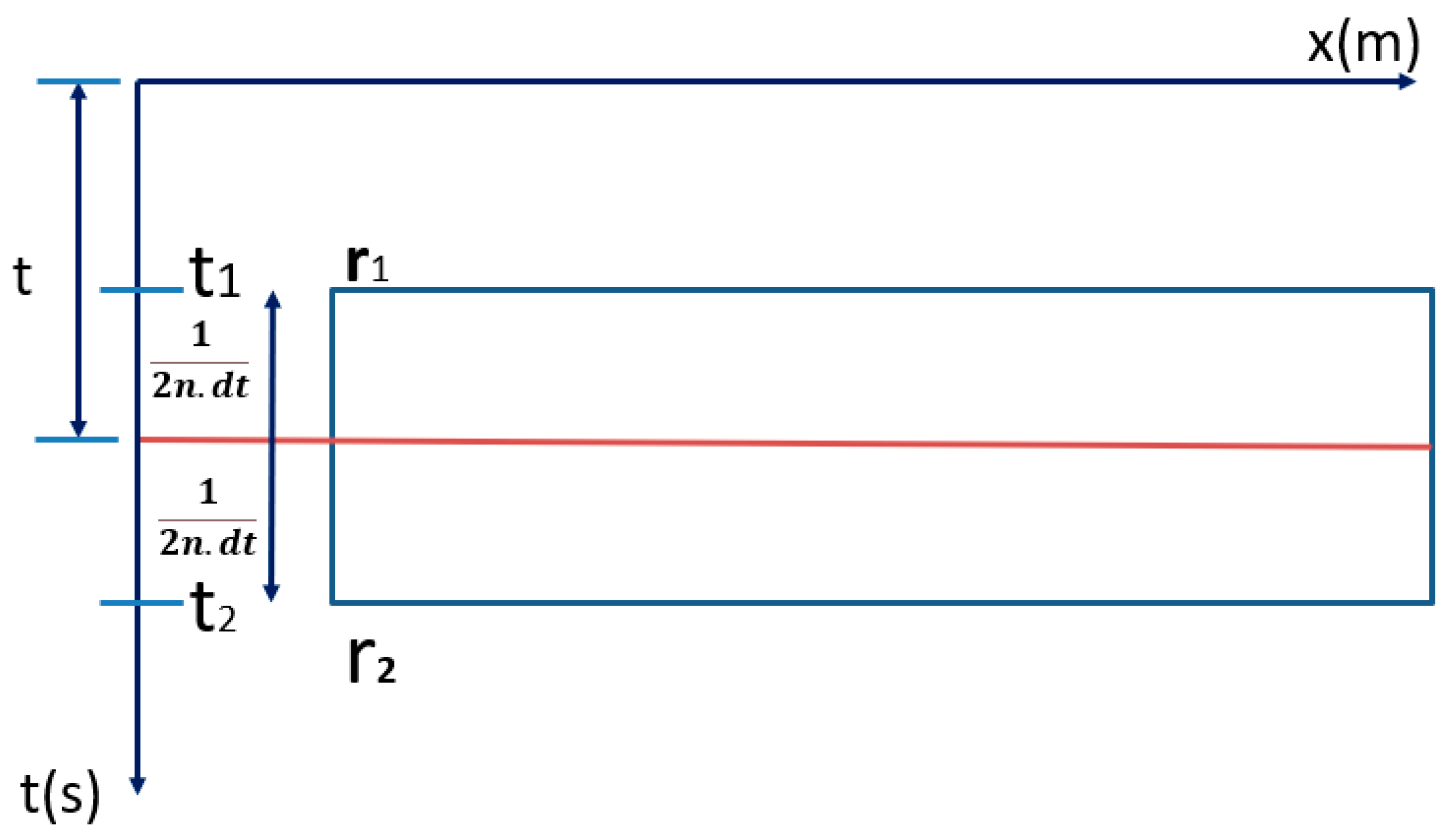
2.2. Reflectivity Spectrum Extrapolation Method

The reflectivity spectrum extrapolation method proposed in this study is aimed at recovering the original earth reflectivity spectrum recorded in the seismic data, which is usually zeroed out by the narrowband wavelets, rather than randomly inventing frequency as in the methods described in Section 2.1 above. The processed seismic data is assumed to be expressed by a simple convolutional model [41] in which the seismic trace, T (s), is the convolution of a constant seismic wavelet (pulse), W, and a reflectivity series, R, plus random noise, n.
T (s) = W*R + n
Figure 5 is an illustration of the convolutional model, in which the geologic section represents the true geology of the formation, and the acoustic impedance log is a product of the density of the geologic elements through which the seismic waves are propagated and the velocity at which it travels through the formations. Although there could be some intra-layer contrasts, acoustic impedance for a single layer is usually assumed to be homogeneous and isotropic. The reflection coefficient is a parameter that describes how much of a wave is reflected at the impedance boundaries and can be expressed as Equation (4):
R c = A i 2 A i 1 A i 2 + A i 1
This model presumes that the subsurface geology is laterally layered [42], with continual rock properties inside those layers, and that reflections are engendered at interface boundaries between those adjacent layers [43], ignoring many waves propagation effects. These are assumed to be fixed during seismic processing. The convolutional model is usually used to create synthetic traces as well as to invert seismic traces into band-limited reflectivity [44]. The bandlimited seismic wavelet causes the problem of geologic reflector resolution by shaping and/or cutting off the higher resolution reflectivity band of the seismic data and returning the spectrum outside the band to zero. In most cases, the wavelet removes both high and low frequencies from the reflected spectrum.
To recover and enhance the true seismic frequencies, the seismic wavelet must be removed by deconvolution processes [14]. It is possible to improve the bandwidth of the seismic data spectrum beyond the original band limit proposed by [5]. This is plausible because seismic data is a transient signal, and all transient signals have an unbounded frequency response that can be predicted to some extent if enough of the spectrum is sampled [4]. To do this, these transient signals must meet two requirements: (1) The spectrum must be simple and distinct, and (2) the signal must have clear frequency periodicities with low noise. Since the reflectivity spectrum is a superposition of sinusoidal layer frequency responses, a blocky earth structure provides a physical basis for valid bandwidth extension [37].
Therefore, any layer with a single reflection coefficient at the top and bottom, as demonstrated by [24] and investigated in detail by [26], can be depicted as an impulse pair reflectivity series. Figure 6 illustrates a two-layer reflectivity model with reflection interfaces at the top and base. The expression (Equation (5)) for an impulse pair in the time domain can be derived from the parameters shown in the figure. This reflection-coefficient pair can be decomposed into even and odd elements, with even elements having an equal magnitude and sign, while the odd components have an equal magnitude but opposite sign [44]. Various layers can be modelled using the weighted sums of the even and odd impulse pair responses.
Q(t) = r1δ (tt1) + r2 δ (tt1n.dt)
where Q(t) is the time domain impulse response or Green’s function, r1 and r2 are the reflectivity at the top and bottom reflectors of the layer, t is time from zero to the corresponding times of r1 or r2, t1 is a time sample at the top reflector, and n.dt = t1 − t2 is the two-way travel-time thickness of the thin bed; δ(t) = the Dirac δ function and is considered for our purpose as a unit impulse at time zero.
The analysis point is usually located at the center of the layer because a phase shift occurs if the analysis window is not centered on the layer [37]. Therefore, Equation (3) can be re-written as follows (See Figure 7):
Q ( t , n )   =   r 1 δ   ( t     1 2 n . d t )   +   r 2   δ   ( t   +   1 2 n . d t )
Spacing between spectral peaks and notches in the frequency domain is precisely the inverse of the layer thickness in the time domain [24,26]. Since layer thickness can be determined robustly from a narrow band of frequencies with a high signal-to-noise ratio, we obtained the frequency spectrum of the impulse pair through a Fourier transform of the time domain impulse pair (Equation (6)), and when simplified by trigonometric identities this is given as Equation (7):
Q(f,n) = 2recos(πf n.dt) + i2rosin(π.f.n.dt)
q(f,n) = 2recos(π.f.n.dt)
q(f,n) = i2ro sin(π.f.n.dt)
The real part (Equation (8)) of the equation corresponds to the even component (re), whereas the imaginary part (Equation (9)) corresponds to the odd component (ro) [34]. The authors of [37] affirmed that the even component constructively interferes as layer thickness approaches zero whereas the odd components interfere destructively as thickness approaches zero. Thus, the even component is more robust against noise as thickness tends towards zero and can be easily used to extend the conventional seismic beyond its original bandwidth [37]. The analysis of peak amplitudes versus bed thickness for each of these components (odd and even) shows that the odd component behaves similarly to the Widess model [34,45]. The maximum amplitude is reached at tuning thickness (λ/4) and then interferes destructively and cancels itself as thickness decreases towards zero (Figure 1). In contrast, the even component becomes more important below λ/8 and behaves just the opposite way [2].
To demonstrate what happens in a general multilayer reflector, the authors of [19] created a sparse reflectivity sequence consisting of three distinct components: a largely even impulse pair, a predominantly odd impulse pair, and a single impulse. The predominantly even reflector pair had a real spectrum with a larger amplitude than the imaginary spectrum and vice versa for the primarily odd pair, whereas the single reflector’s real and imaginary spectrums were of the same amplitude, but they were one-quarter of the spectral period apart. This suggested that the individual components respond differently to reflectors, and their spectra can be linearly summed up to obtain a composite reflectivity spectrum (See Figure 8). Using dipole decomposition, the reflector pair can be further decomposed into a unit even pair ( 1 2 n . d t ) and a unit odd pair ( 1 2 n . d t ) weighted by coefficients re and ro, respectively. The two reflection coefficients for the impulse pair can thus be represented as (re + ro) and re − ro, either of which ranges from −1 to 1 and could be zero denoting a single impulse. The frequency spectrum of the impulse pairs can be calculated from Equations (8) and (9).
Any missing frequency outside the original bandwidth can be computed using Equation (7) below [39], assuming that K is the number of impulse pairs in the analysis window (including zero), while n varies from zero to the number N to accommodate all bed thicknesses and dt is the sample rate. The broadband spectrum which can range from zero to the Nyquist frequency (i.e., the maximum frequency that can be observed in the data) of any reflectivity series within the analysis window can be clearly expressed as:
S r ( f ) = n = 0 k 1 ( 2 r e ( n ) . c o s ( 2 π . n . d t . f )   +   i 2 r 0 ( n ) . s i n ( 2 π . n . d t . f )
In this study, the coefficients (re) and (ro) components were computed using the basis pursuit inversion algorithm proposed by [17,21]. Many methods for spectral decomposition have been previously described and analyzed by [28,46,47,48]. Spectral decomposition is non-unique, and each method has advantages and disadvantages. To use the spectral analysis for layer thickness estimation, precision is needed in both the frequency domain (in order to resolve the thickness) and in the time domain (in order to predict its location in time). Thus, the inversion-based basis pursuit decomposition (BPD) was used for this analysis. This technique proposes that since the sample rate is dt, each trace of even reflectivity consists of a pair of equal impulse functions (spikes) with interval n.dt [17]. The reflector kernel matrix for the reflectivity pair is constructed by shifting the reflectivity pair along the time axis with m.dt, where m ranges from 1 to the maximum number of samples in the seismic trace [17]. So, each even (re) and odd (ro) reflectivity are given in time domain as Equations (11) and (12) respectively.
re(t m, n, Δt) = δ (tm.dt) + δ(tm.dt + n.dt)
ro(t m, n, Δt) = δ (tm.dt) − δ(tm.dt + n.dt)
For our purpose, this same operation was applied in the frequency domain to compute the even and odd impulse pairs. A sum of frequency sinusoids multiplied by the wavelet spectrum is the narrowband data spectrum, which is associated with a sum of reflector pairs. The convolution of reflectivity with seismic wavelets in the time domain is equivalent to multiplication with wavelet spectrum in the frequency domain [49]. Therefore, to obtain reflectivity in the frequency domain, the seismic data spectrum (in the frequency domain) is divided by a known or pre-estimated wavelet spectrum. Since the wavelet is known, the reflectivity spectrum of the bandlimited data is obtained by dividing it by the wavelet spectrum [50].
This produces a flattened spectrum, which corresponds to the wavelet spectral limit section of the broadband reflectivity spectrum obtained using Equation (10), and a best-fit sinusoid is readily fitted to these amplitude points. It is then easy to extrapolate the layer reflectivity spectrum outside the original seismic band by extending the spectra sinusoid (Figure 9).
The forward modeling of the data spectral constraint (real part and imaginary part separately) and the sinusoidal elements of varying frequency periodicities now within the same spectral limit can be given as Equation (13):
φ = βα + ε
where φ is the deconvolved data spectrum, β is the kernel matrix of sinusoidal atoms, α is the reflection coefficients vector including re and ro, and ε denotes the prediction error [19,38]. The kernel has a dimension of µ × K, where µ is the number of frequencies determined by the available bandwidth and the sampling rate in frequency, K is the number of layers and hence the number of even or odd pairs stated by Equation (10) above, and can be varied to encompass all possible frequency periodicities.
By solving the objective function (Equation (14)), basis pursuit concurrently minimizes both the L2 norm of the error term and the L1 norm of the solution, creating sparsity in the solution vector. The L1 norm is defined as the sum of the seismic trace’s absolute values. The square root of the sum of the squares of the seismic trace values is the L2 norm, on the other hand. The parameters are solved using linear programming.
min [||φβα ||2 + λ||m||1]
Lambda (λ) in Equation (14) is the trade-off parameter between sparsity and accuracy of the solution. The regularization parameter λ balances the inverted reflectivity resolution and noise. Increasing λ decreases the resolution of inverted reflectivity and decreasing λ may cause noise amplification [17,51]. In this study, the λ value was determined empirically.
After the bandwidth is extended, we can calculate the resulting reflectivity series by inverting the reflectivity spectrum (in the frequency domain) to the time domain using Equation (15) [20,52], since it shares the same coefficient with Equation (10).
S r ( t ) = n = 0 k 1 ( ( r e ( n ) + r o ( n ) ) b ( t + n . d t ) + ( r e ( n ) r o ( n ) ) b ( t n . d t ) )      

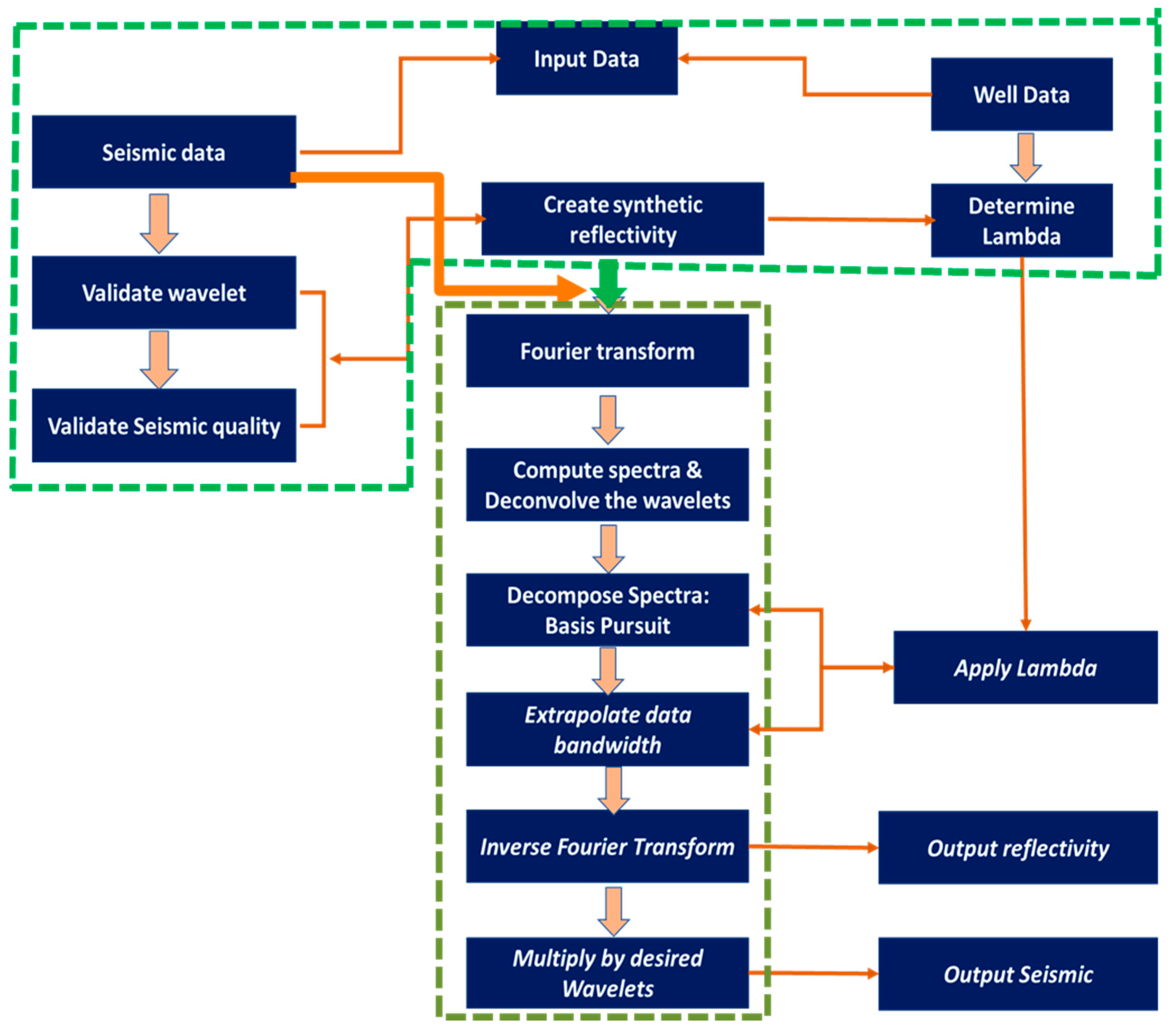
2.3. Summary of the Adopted Method

Figure 10 illustrates the algorithmic scheme of the applied techniques. To implement the harmonic extrapolation algorithm, it was ensured that some of the critical assumptions stated above hold for the seismic data used. First, the bandlimited seismic was correlated to two wells to understand the characteristics of the wavelet response. This was necessary because we extrapolated from the known (bandlimited) frequency to the unknown (extrapolated band). By comparing the synthetic to the seismic data, we ascertained the signal-to-noise ratio of the data; noisy data would amount to noise boosting. The sample rate of the data is 2 ms, which was judged to be sufficient and would give a good output frequency band. To ensure that noise was not introduced into the data, an acceptable regularization parameter of 0.01 was selected by comparing the well resolution to the seismic. For each seismic trace, an analysis window was slid along the trace to compute the Fourier transform at every window location. We divided the spectra by the wavelet spectrum to deconvolve the reflectivity spectrum. Furthermore, a basis pursuit atomic algorithm was applied to decompose the real and imaginary parts of the spectrum into summations of cosines and sines. Finally, we extrapolated the decomposed sinusoids to the band of interest, multiplied by the desired output wavelet spectrum, and inversed the Fourier transform to get a time reflectivity series associated with each window position. The addition of the time series overall window positions formed the bandwidth-extended trace.

3. Results

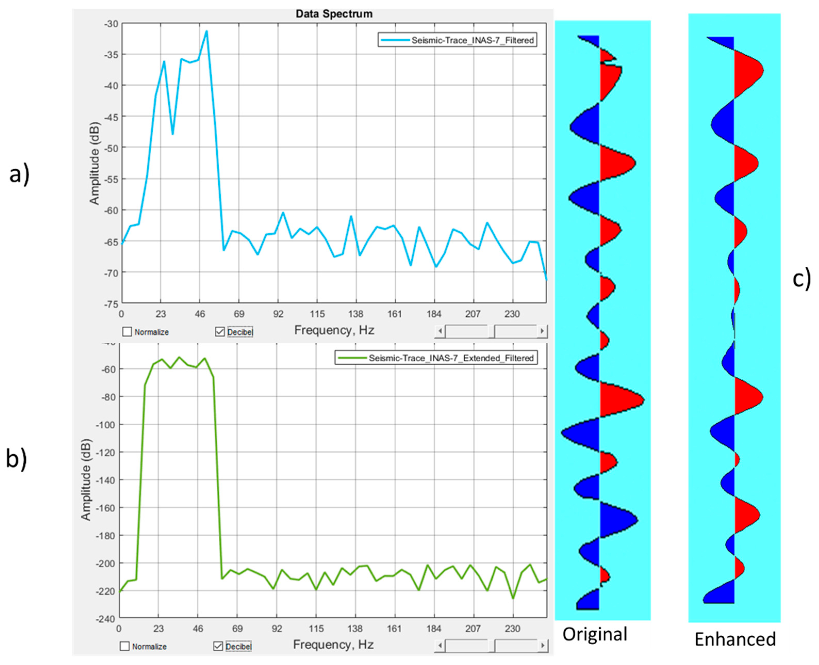
3.1. Test of the Algorithm on the Seismic Trace Model

A seismic trace model was built to test the efficacy of the harmonic extrapolation algorithm before applying it to real seismic data. The thickness of the model was determined from the E reservoir (of Inas Field), which is encased in between shales. Upon definition of this interval, shear wave velocity, compressional wave velocity, and the density of the reservoir were used to model a synthetic reflectivity series, and a statistical wavelet was extracted at a time interval corresponding to the reservoir zone. The vertical time thickness of the model is 200 ms (600 ms–800 ms), and its amplitude range is −0.22 to +0.22. The time thickness of the individual loops of the trace ranges from 11 ms to 27 ms. See Figure 11 below.
A basis pursuit decomposition algorithm was applied to the modeled trace to decompose it into a superposition of layer spectra [17], and the emerging components were summed up using Equation (10) to obtain the band expanded trace shown in Figure 12 below. The result shows an improved resolution while also maintaining the characteristics of the original trace. It is observed that the seismic amplitude is reduced significantly across the time series. For instance, the maximum positive amplitude dropped from +0.2 to +0.053 while the maximum negative amplitude increased from −0.2 to −0.068. To correct for the amplitude difference, a global factor was applied by multiplying the amplitude by a constant, and the result is as shown in Figure 13 below, which is an overlay of both traces. Both traces compare very well, while the enhanced trace also maintains a very good resolution.
The time thickness resolution is sufficient, allowing very thin layers to be resolved within the modeled interval. The loop’s minimum resolvable time thickness fell from 11 ms to 2 ms. The bandwidth of the original seismic model was estimated to be around 68 Hz, as illustrated in Figure 14. Using the extrapolation methods described above, its bandwidth increased from 68 Hz to 161 Hz (Figure 10), a 137 (((161 − 68)/68) × 100) percent increase.
The amplitude spectrum of the enhanced trace between 15 Hz and 68 Hz (bounded by the dashed red lines) mirrors that of the original normalized spectrum (Figure 14), however with a slightly different amplitude magnitude. The spectrum of the original trace is a composite of the unit impulse pairs. Due to the limitedness of the seismic impulse, this often causes a destructive interference of thin reflectors, thereby resulting in unrealistically high amplitudes. When a signal correctly resolves a layer, the impulse pairs (top and base) of the reflectors constructively interferes, retaining the correct amplitude. This suggests why the amplitude of 9a and 9b defers after signal processing. Notice that the spectrum of the enhanced signal has more notches, which indicates that more layers were resolved, whereas the spectrum of the original data has those layers lumped up in few notches. The outlined portion depicts the sampled component utilized to expand the frequency to beyond the original band limit. The extrapolation’s validity is determined by how accurately the sampled component of the original data is represented in the enhanced data. As a result, data quality must be meticulously validated using the procedure described above. Bandwidth extension to 161 Hz frequency helped to resolve the reflections at about 2–11 ms time thickness and sharpened the events, as shown in Figure 12. The initial model (Figure 11) is fairly like the enhanced trace, albeit not identical as one might assume due to the added frequency.
Apart from the visual representation discussed above, the impact of the algorithm was assessed by filtering off the extra frequency. Frequency domain filtering is a common practice in seismic data processing [53,54,55,56,57,58]. Both data sets were put through the same frequency cuts (10 Hz, 30 Hz, 45 Hz, and 60 Hz) to see how well they matched [46]. They compared favorably, as shown in Figure 15, with only slight variances. This demonstrates that the modified seismic trace can be used to reconstruct the original one. The fact that they are so closely related implies that the procedure was effective.
In comparison, the enhanced trace has a better correlation with the acoustic impedance and well reflectivity series. Figure 16 shows a plot of the acoustic impedance (AI) contrast of the geologic reflectors, the reflection coefficients (RC) responses at the interface boundaries, and both seismic traces. The original trace captures the reflectivity layers sparingly, whereas the enhanced trace resolved more thin layers. The original trace clumped several resolvable spikes into a single loop, obscuring the geologic information they represented.

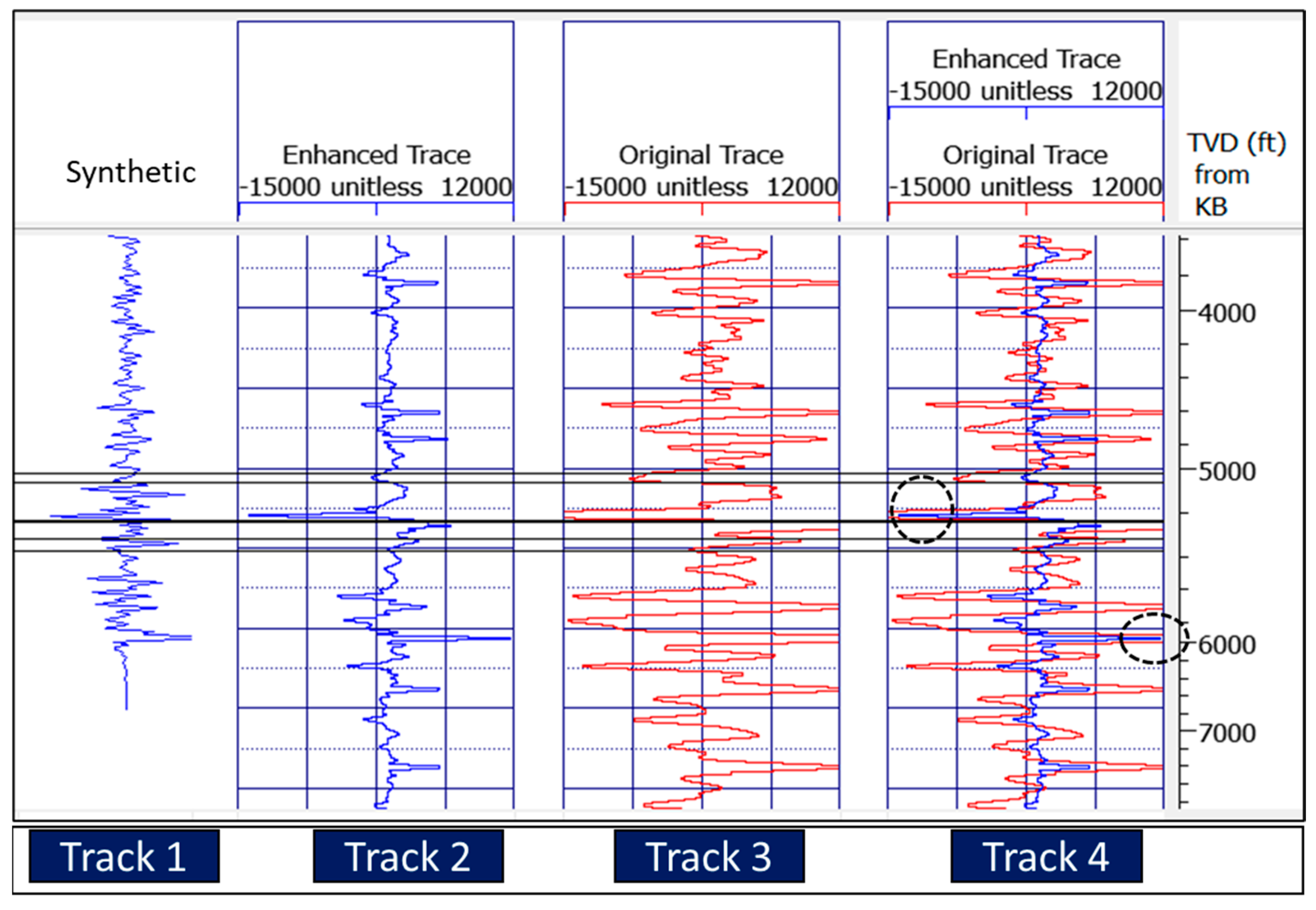
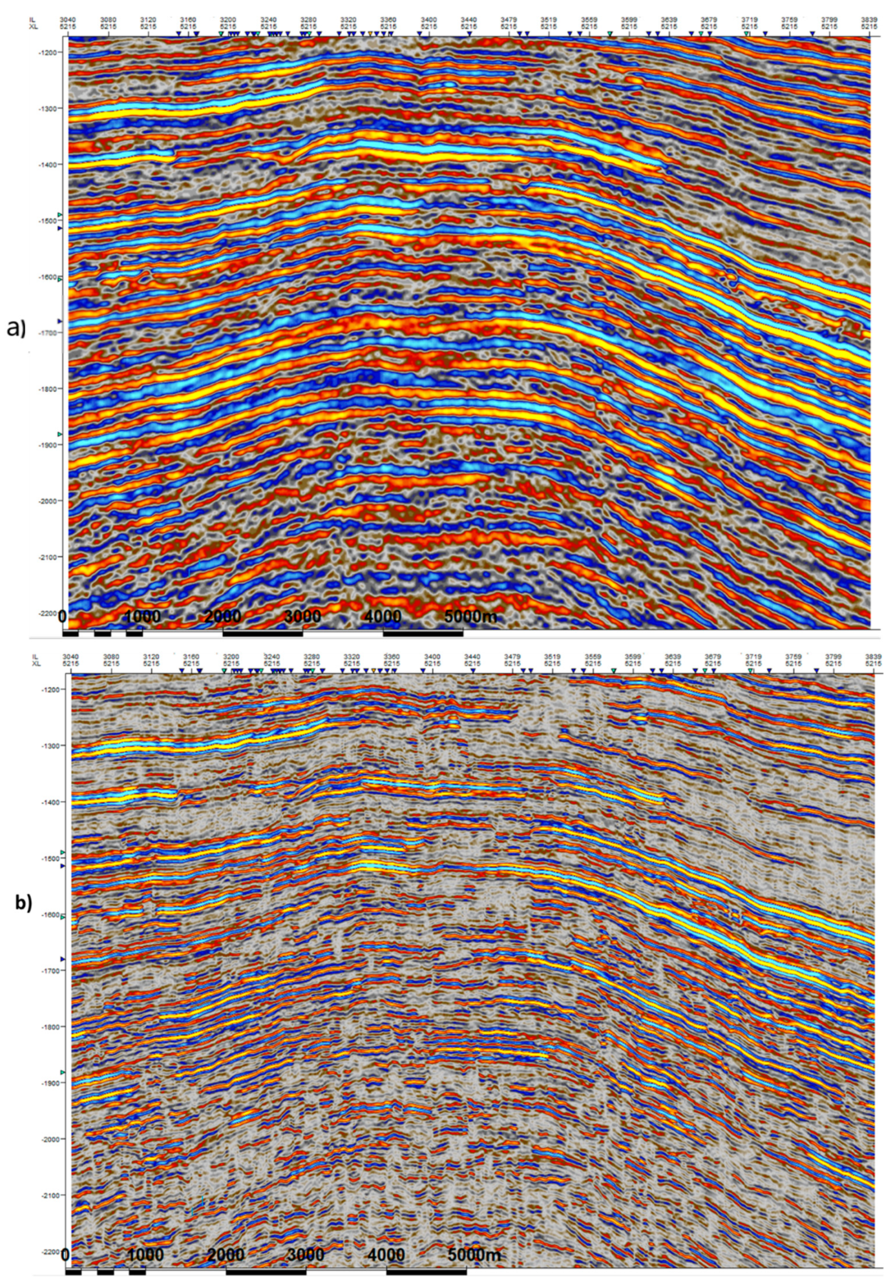
3.2. Test of the Algorithm on Real Seismic Data

Spectral analysis was done to understand the seismic data spectral properties as part of the data quality control process. The seismic data is zero phased with a positive reflection coefficient for high impedance layers. The bandwidth of the wavelet was determined to be 80 Hz from the spectral plot. The peak frequency of the data ranges from 22 Hz to 35 Hz, while the dominant frequency is 31 Hz. Several wavelets were extracted from the seismic and wells by varying the frequencies, time windows, and frequency filtering algorithms. The same procedure described for the synthetic trace model above was applied to the entire volume, which resulted in an expanded bandlimit of 170 Hertz as shown in Figure 17 below.
The seismic trace at the well (Inas-1) intersection was extracted from both the enhanced and original trace for further comparison. In Figure 18, the synthetic seismogram generated from the same well was compared to both traces. The enhanced trace (Track 2) has a shorter wavelength, better resolution, and a stronger correlation to the synthetic seismogram (Track 1) than the original trace (Track 3). An overlay of both traces on the same track (Track 4) reveals a considerable difference in the magnitude of the reflection strengths (reflection coefficients), with the exception of a few reflectors where the magnitudes are equal, as indicated by the dotted black circles.
At the reservoir interval, the resolution limit (or tuning thickness) of the seismic data was calculated to be roughly 31 m. Upon application of the algorithm, the resolution limit was substantially reduced to 10 m without changing the real reflection signals as shown in Figure 19a,b.
Figure 20 also shows the seismic sections from the original (A) and improved (B) data. For instance, Figure 20B displays a channel-filled deposit (enclosed by the dotted red circle), whereas the channel is clearly hidden in Figure 20A due to insufficient resolution. Unresolved thin beds in the bandlimited data are shown to be well-resolved in the improved data (compare the white arrows in both sections, A & B). The composite trace blends the thin layer with other layers into a single loop when a bed is below the seismic tuning thickness. The dotted green arrow in Figure 20B indicates a stratigraphic pinch-out, but looks continuous in Figure 20A.

3.3. Spectral Decomposition of the High and Low-Frequency Data

The output of spectral decomposition is characterized by more localized anomalies, which increases the details of interpretation and makes it possible to obtain detailed results from the seismic data. Figure 21 demonstrates the improvement of the enhanced data over the original. It shows the results of a generalized spectral decomposition (GSD) applied on both the original and enhanced seismic data. For a fair comparison, we used the RGB (red, blue, and green) blending algorithm to mix frequency volumes of 10 Hz, 30 Hz, and 40 Hz derived from both data. Time slices of the respective seismic volumes were taken at different time depths to visualize the geologic information in the data. Spectral decomposition is a tool for better imaging and mapping temporal bed thickness and geological discontinuities within 3D seismic surveys [18], and it aids in seismic interpretation by analyzing the variation of amplitude spectra and phase spectra. Amplitude spectra delineate thin-bed variability via spectral notching patterns that can be used to map the subtle stratigraphic changes such as channel systems [28]. It can be observed from the figures below that the original seismic data has smeared and fuzzy appearance, whereas the features in the improved data are sharp and distinct. Figure 21 shows a clastic depositional system in a predominantly fluvial-deltaic environment in Inas Field, offshore Malay Basin. Although the traces of some geologic features are faintly visible in Figure 21a, it is hard to interpret the geologic history prevalent in the field. As indicated in Figure 21b below, we were able to interpret the entire depositional system using the enhanced data. It was easier to see the geologic stories in the data. The whole depositional system is visible, and how the river channel prograded from the hinterland, through the coastal plain to the delta plain, is seen. Subtle features such as the barrier complexes, alluvial fan system, crevasse splay, point bar system, coastal planes, and chute-cut oxbow lakes are well resolved with their correct geomorphologies conspicuously shown.

4. Discussion

The results presented above demonstrate the importance of improving seismic data resolution. The authors of [20] aptly posited that since the seismic trace is a superposition of many overlapping reflections, it is often difficult to identify the exact reflection boundaries. The applied harmonic extrapolation algorithm enhanced the frequency content of the data and made subtle geologic features more easily identifiable. As illustrated by Figure 20 and Figure 21, the enhanced seismic data shows a significant increase in resolution resulting in detailed reservoir stratigraphy, clearer pinch outs, and structures as the event appeared more sharply defined and less affected by low-frequency noise (David et al., 2020). In agreement with Gurley and Kareem, 1990, this increment in resolution was possible because wavelet transformation allows the retention of local transient signal characteristics beyond the capabilities of the infinite harmonic basis functions by allowing a multi-resolution representation of a process. The recovery of this transient signal formed the basis for the enhanced resolution of the sub-seismic features presented above, not the arbitrary invention of frequency [19], suggesting the recoverability of seismic frequency below the conventional tuning limit.
Moreover, the observed reduction of signal amplitude in Figure 12 and Figure 18 for the trace model and the seismic trace, respectively, could give an insight into what happens in the resolution of thick and sub-seismic features. Further, ref. [6] hinted that the differences between thin-bed response and thick-bed response are that thick-bed response has a separate response for the top and bottom of the bed, the two wavelets do not interfere substantially, and the amplitude of the wavelet depends on reflection strength (reflection coefficient). For isolated thin beds, reflections from the top and bottom of the bed interfere. The result is a single wavelet response that approximates the time derivative of the original wavelet. This implies that the amplitude response of a thin bed in narrowband data is not a true response of the bed thickness, but an approximation of the amplitude responses of the interfered wavelets. Thus, it is assumable that when the thin bed is correctly resolved, the actual amplitude responses are reinstated. This explains the reduction in amplitude magnitude after we applied the enhancement algorithm. The thin beds are diminished in amplitude according to the thinness of the bed. An advantage of having this enhanced data is that thin beds are more correctly resolved, and the interference problems are less disruptive. High-frequency enhancement aims to sharpen the data, apparently by better defining structures and pinch-outs [18]. They can aid interpretation by making events appear more markedly defined and less deluged by the low-frequency ringing that characterizes conventional seismic data [59].
Figure 14 and Figure 17 illustrate that the bandwidth of both the trace model and the seismic data spectra were increased by about 137% respectively. This increment translated to increased resolutions as shown in other results above, suggesting that resolution is directly proportional to the bandwidth of the wavelet. The broader the bandwidth, the greater the resolution [6]. Thus, it is safe to say that resolution depends directly on bandwidth and indirectly on frequency.
We hereby affirm that in the harmonic extrapolation of the bandwidth of Inas seismic data, we have illustrated that the time domain impulse pair of geologic reflectors can be decomposed into odd and even parts in the frequency domain, which can be further inverted by dividing out the overprinted wavelets with a known seismic pulse response to recover the earth’s reflectivity spectra and further re-inversed to the time domain as broadband seismic data [51,60,61]. A test of this method using a synthetic trace constructed from input well logs shows that the seismic bandwidth can be extended using this scientific approach without necessarily boosting noise. When applied to real seismic data, the resolution of geologic features such as sub-seismic faults, channels, and thin beds is improved. By spectrally decomposing the original and enhanced seismic data and comparing the results, we demonstrated that paleo-geomorphologic features and subtle stratigraphic geomorphologies such as crevasse splay, oxbow lakes, point bars, barrier bar, lagoon elements, and faintly facies variations can be easily interpreted using the improved data.

5. Conclusions

By the harmonic extrapolation of the Inas Field seismic reflectivity spectrum, we have demonstrated the recovery of the original earth’s reflectivity spectrum usually zeroed out by the wavelets. Based on the new insights drawn from the results of this research, we hereby conclude that
  • it is possible to recover the earth’s reflectivity spectrum from the seismic data by harmonically extending the bandwidth of the data spectrum, because wavelet deconvolution allows the retention of local transient signal characteristics beyond the capabilities of the infinite harmonic basis functions;
  • to correctly resolve the thin geologic features, the amplitude magnitude is diminished according to the thinness of the feature., thereby removing the effects of destructive interference that projects incorrect amplitudes;
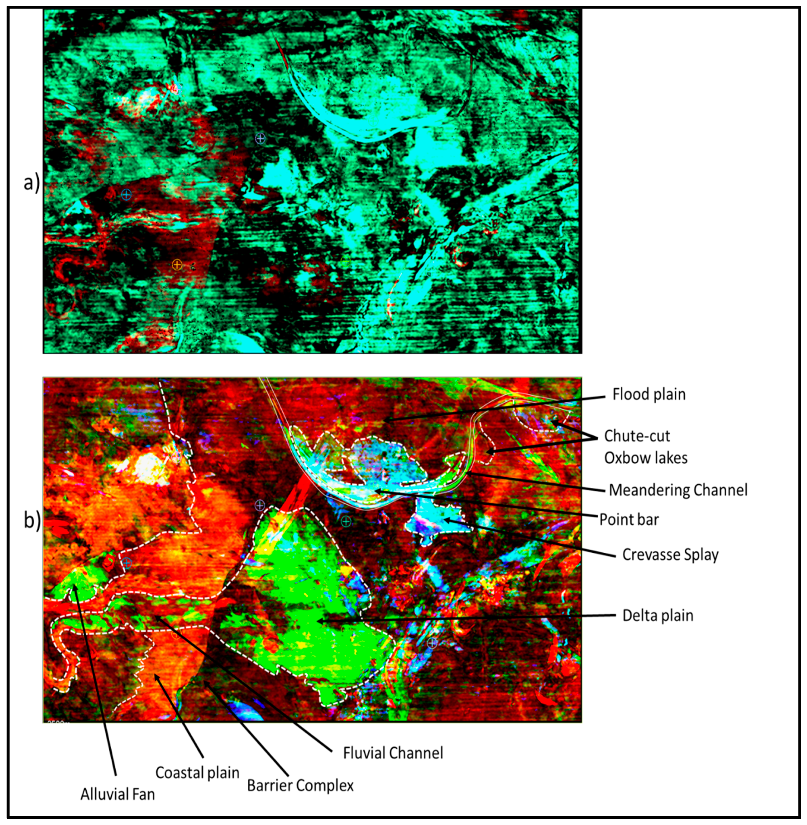
  • the harmonic bandwidth extension technique significantly improved the resolutions of the input seismic data and revealed subtle geologic features such as meandering channels, crevasse splay, oxbow lakes, chute-cut, point bars, barrier bar, alluvial fan, and other lagoon elements, thereby suggesting the applicability of this method for detailed stratigraphic studies.
It is important to note that the results presented in this research are based on the application of this method in Inas Field, Offshore, Northern Malay Basin, and may vary in other geologic settings. Therefore, a further test of this technique in other basins is highly recommended.
Applications:
(1)
This technique can be applied to investigate the connectivity, continuity, and individuality of reservoir facies, since it enables the imaging of subtle geologic details [39].
(2)
The authors of [39] demonstrated that the geostatistical inversion of broadband seismic data can give an accurate prediction of facies extent in a hydrocarbon reservoir. The findings of [62] also revealed that the amount of CO2 storage and enhanced oil recovery is dependent on the pore size distribution, which is indirectly dependent on the reservoir rock facies. Hence, a broadband seismic obtained through the techniques presented in this research can be applied to predict the extent of reservoir rock facies, in an unconventional CO2 storage [63,64,65].
Further Research:
(1)
It is unclear whether reducing amplitude magnitudes influences the response of thick beds, or whether this technique affects how amplitude varies with offset (AVO) and other attributes, especially in hydrocarbon reservoirs. Therefore, the authors suggest that more research be done to see how this technique impacts seismic attributes.
(2)
The fact that this technique requires a lot of time, space, and processor speed to run is a disadvantage; however, future research can work on lowering the processing needs.

Author Contributions

The Conceptualization, methodology, formal analysis, data curation, and the original draft preparation of this manuscript were done by B.O.N., whereas the review and editing, validation, supervision, project administration, and funding acquisition, were done by M.H. All authors have read and agreed to the published version of the manuscript.

Funding

This research was funded by Yayasan Universiti Teknologi PETRONAS (YUTP), grant number: 015LC0-414.

Data Availability Statement

PETRONAS Malaysia provided the data that supported the study’s findings. Restrictions apply to the availability of these datasets, which were used under license for this study. Data is available from the authors with the permission of PETRONAS.

Acknowledgments

The authors are glad to express their profound appreciation to PETRONAS for providing the data used for this study. Our gratitude also goes to Lumina Geophysical Houston, CGG, and Schlumberger for their immense contribution towards the success of this work by giving us a free license to their software, which was used on different occasions to achieve the results presented in this research. Not forgetting the Universiti Teknologi PETRONAS, without whom this work would not have been possible for providing the facilities used in this research.

Conflicts of Interest

The authors declare no conflict of interest. We affirm that there is no personal circumstances or interest that may be perceived as inappropriately influencing the representation or interpretation of the reported research results. The funders had no role in the design of the study; in the collection, analyses, or interpretation of data; in the writing of the manuscript, or in the decision to publish the results.

References

  1. Zeng, H. Seismic Imaging for Seismic Geomorphology beyond the Seabed: Potentials and Challenges; Special Publications; Geological Society: London, UK, 2007; Volume 277, pp. 15–28. [Google Scholar] [CrossRef]
  2. Chopra, S.; Castagna, J.; Portniaguine, O. Seismic Resolution and Thin-Bed Reflectivity Inversion, Arcis Corporation, Calgary; Fusion Petroleum Technologies, Inc.: Houston, TX, USA; University of Houston: Houston, TX, USA, 2006; pp. 19–23. [Google Scholar]
  3. Herron, A.D. First Steps in Seismic Interpretation; Society of Exploration Geophysicists: Houston, TX, USA, 2011; pp. 75–81. [Google Scholar]
  4. Gurley, K.; Kareem, A. Applications of wavelet transforms in earthquake, wind and ocean engineering. Eng. Struct. 1999, 21, 149–167. [Google Scholar]
  5. Sheriff, R.E. Encyclopedic Dictionary of Applied Geophysics, 4th ed.; Society of Exploration Geophysicists: Houston, TX, USA, 2002. [Google Scholar]
  6. Knapp, R.W. Vertical resolution of thick beds, thin beds, and thin-bed cyclothems. Geophysics 1990, 55, 1942–2156. [Google Scholar] [CrossRef]
  7. Simm, R.; Bacon, M. Seismic Amplitude, an Interpreter’s Handbook; Cambridge University Press: Cambridge, UK, 2014; pp. 32–36. [Google Scholar]
  8. Widess, M.B. How thin is a thin bed? Geophysics 1973, 38, 1176–1180. [Google Scholar] [CrossRef]
  9. Francis, A. A Simple Guide to Seismic Amplitudes and Detuning. Geo ExPro Mag. 2015, 12, 68–78. [Google Scholar]
  10. Roden, R.; Smith, T.A.; Santogrossi, P.; Sacrey, D.; Jones, G. Seismic interpretation below tuning with multiattribute analysis. Lead. Edge 2017, 36, 330–339. [Google Scholar] [CrossRef]
  11. Paternoster, B.; Cauquil, E.; Saint-André, C. How good seismic resolution needs to be for detecting thin beds? In Proceedings of the Offshore Technology Conference, Houston, TX, USA, 2 May 2011; pp. 1–5. [Google Scholar]
  12. Koefoed, O. Aspects of vertical seismic resolution. Geophys. Prospect. 1981, 29, 21–30. [Google Scholar] [CrossRef]
  13. Zabihi Naeini, E.; Sams, M.S. Accuracy of Wavelets, Seismic Inversion, and Thin-Bed Resolution, Society of Exploration Geophysicists and American Association of Petroleum Geologists. Interpretation 2017, 5, T523–T530. [Google Scholar] [CrossRef] [Green Version]
  14. Kirchberger, L. Enhancing vertical seismic resolution by spectral inversion. Soc. Pet. Eng. 2012, 1–5. [Google Scholar] [CrossRef]
  15. Hargreaves, N.; Calvert, A. Inverse Q filtering by Fourier transform. Geophysics 1991, 56, 519–527. [Google Scholar] [CrossRef]
  16. Fraser, G.B.; Neep, J. Increasing seismic resolution using spectral blueing and colored inversion: Cannonball field, Trinidad. In Proceedings of the 74th Annual International Meeting, SEG, Expanded Abstracts, Denver, CO, USA, 10–15 October 2004; pp. 1794–1797. [Google Scholar] [CrossRef]
  17. Zhang, R.; Castagna, J.P. Seismic sparse-layer reflectivity inversion using basis pursuit decomposition. Geophysics 2011, 76, R147–R158. [Google Scholar] [CrossRef] [Green Version]
  18. Young, P.; Wild, A. Cosmetic enhancement of seismic data by loop re-convolution. In Proceedings of the CSEG Convention, Expanded Abstracts, Calgary, AB, Canada, 16–19 May 2005; pp. 78–80. [Google Scholar]
  19. Liang, C.; Castagna, J.P.; Zavala, R.T. Tutorial: Spectral bandwidth extension—Invention versus harmonic extrapolation. Geophysics 2017, 82, W1–W16. [Google Scholar] [CrossRef]
  20. Kumar, S.; Kumari, K.; Biswal, A. Frequency Enhancement of Seismic Data—A comparative study. CSEG Rec. 2008, 33, 38–43. [Google Scholar]
  21. Chen, S.S.; Donoho, D.L.; Saunders, M.A. Atomic decomposition by basis pursuit. Soc. Ind. Appl. Math. Rev. 2001, 43, 129–159. [Google Scholar] [CrossRef] [Green Version]
  22. Barnes, A.E. A tutorial on complex seismic trace analysis. Geophysics 2007, 72, W33–W43. [Google Scholar] [CrossRef]
  23. De Abreu, E.; Jarrah, F.; Aboro, O.; Aziz, A.S. The use of spectral decomposition to QC seismic data. In Proceedings of the SEG international Exposition and 87th Annual Meeting, Houston, TX, USA, 24–27 September 2017; pp. 2169–2173. [Google Scholar]
  24. Partyka, G.; Gridley, J.; Lopez, J. Interpretational applications of spectral decomposition in reservoir characterization. Lead. Edge 1999, 18, 353–360. [Google Scholar] [CrossRef] [Green Version]
  25. Brown, A.R.; Partyka, G.A.; Bush, M.D.; Garossino, P.G.A.; Gutowski, P.R. Spectral decomposition. In Interpretation of Three-Dimensional Seismic Data, 7th ed.; Brown, A.R., Ed.; AAPG Memoir 42 and Society of Exploration Geophysicists Investigations in Geophysics 9; Society of Exploration Geophysicists: Houston, TX, USA, 2011; pp. 283–308. [Google Scholar] [CrossRef]
  26. Marfurt, K.J.; Kirlin, R.L. Narrow-band spectral analysis and thin-bed tuning. Geophysics 2001, 66, 1274–1283. [Google Scholar] [CrossRef] [Green Version]
  27. Goloshubin, G.M.; Korneev, V.A.; Vingalov, V.M. Seismic low-frequency effects from oil-saturated reservoir zones. In Proceedings of the 72nd Annual International Meeting of the Society of Exploration Geophysicists, Salt Lake City, UT, USA, 6–11 October 2002; pp. 1813–1816. [Google Scholar] [CrossRef] [Green Version]
  28. Castagna, J.; Sun, S.; Siegfried, R.W. Instantaneous spectral analysis: Detection of low-frequency shadows associated with hydrocarbons. Lead. Edge 2003, 22, 120–127. [Google Scholar] [CrossRef]
  29. Sinha, S.; Routh, P.S.; Anno, P.D.; Castagna, J.P. Spectral decomposition of seismic data with continuous-wavelet transform. Geophysics 2005, 70, P19–P25. [Google Scholar] [CrossRef]
  30. Welsh, A.; Brouwer, F.G.C.; Wever, A.; Flierman, W. Spectral decomposition of seismic reflection data to detect gas-related frequency anomalies. In Proceedings of the 70th European Association of Geoscientists and Engineers Conference and Exhibition, Rome, Italy, 9–12 June 2008; pp. 263–267. [Google Scholar] [CrossRef]
  31. Saeid, E.; Kendall, C.; Kellogg, J.; De Keyser, T.; Hafiz, I.; Albesher, Z.; Martinez, J.A. A depositional model for the Carbonera Formation, Llanos Foothills, Colombia, from workflow of a sequence stratigraphic framework and interpretation from well-log stacking patterns, well cuttings, and three-dimensional seismic spectral decomposition. AAPG Bull. 2022, 106, 321–353. [Google Scholar] [CrossRef]
  32. Chopra, S.; Marfurt, K.J. Choice of mother wavelets in CWT spectral decomposition. In SEG Technical Program Expanded Abstracts 2015; Society of Exploration Geophysicists: Houston, TX, USA, 2015; pp. 2957–2961. [Google Scholar]
  33. Mora, D.; Castagna, J.; Meza, R.; Chen, S.; Jiang, R. Case study: Seismic resolution and reservoir characterization of thin sands using multiattribute analysis and bandwidth extension in the Daqing field, China. Interpretation 2020, 8, T89–T102. [Google Scholar] [CrossRef]
  34. Tirado, S. Sand Thickness Estimation Using Spectral Decomposition. Master’s Thesis, University of Oklahoma, Norman, OK, USA, 2004; 63p. [Google Scholar]
  35. Castagna, J.P. Spectral decomposition and high-resolution reflectivity inversion. In Proceedings of the CSEG National Convention, Calgary, AB, Canada, 16–19 May 2005. [Google Scholar]
  36. Portniaguine, O.; Castagna, J.P. Spectral inversion: Lessons from modelling and Boonesville case study. In SEG Technical Program Expanded Abstracts 2005; Society of Exploration Geophysicists: Houston, TX, USA, 2005; pp. 1638–1641. [Google Scholar]
  37. Puryear, C.; Castagna, J.P. Layer-thickness determination and stratigraphic interpretation using spectral inversion: Theory and application. Geophysics 2008, 73, R37–R48. [Google Scholar] [CrossRef]
  38. Madon, M.B.H. Depositional setting and origin of berthierine oolitic ironstones in the lower Miocene Terengganu shale, Tenggol Arch, offshore peninsular Malaysia. J. Sediment. Petrol. 1992, 65, 899–916. [Google Scholar]
  39. Nwafor, B.O.; Hermana, M.; Elsaadany, M. Geostatistical inversion of spectrally broadened seismic data for re-evaluation of oil reservoir continuity in Inas field, offshore Malay Basin. J. Mar. Sci. Eng. 2022, 10, 727. [Google Scholar] [CrossRef]
  40. Madon, M.; Abolins, P.; Hassan, R.A.; Yakzan, A.M.; Yang, J.S.; Zainal, S.B. Petroleum systems of the Northern Malay Basin. Pet. Geol. Conf. Exhib. Bull. 2004, 49, 125–134. [Google Scholar] [CrossRef] [Green Version]
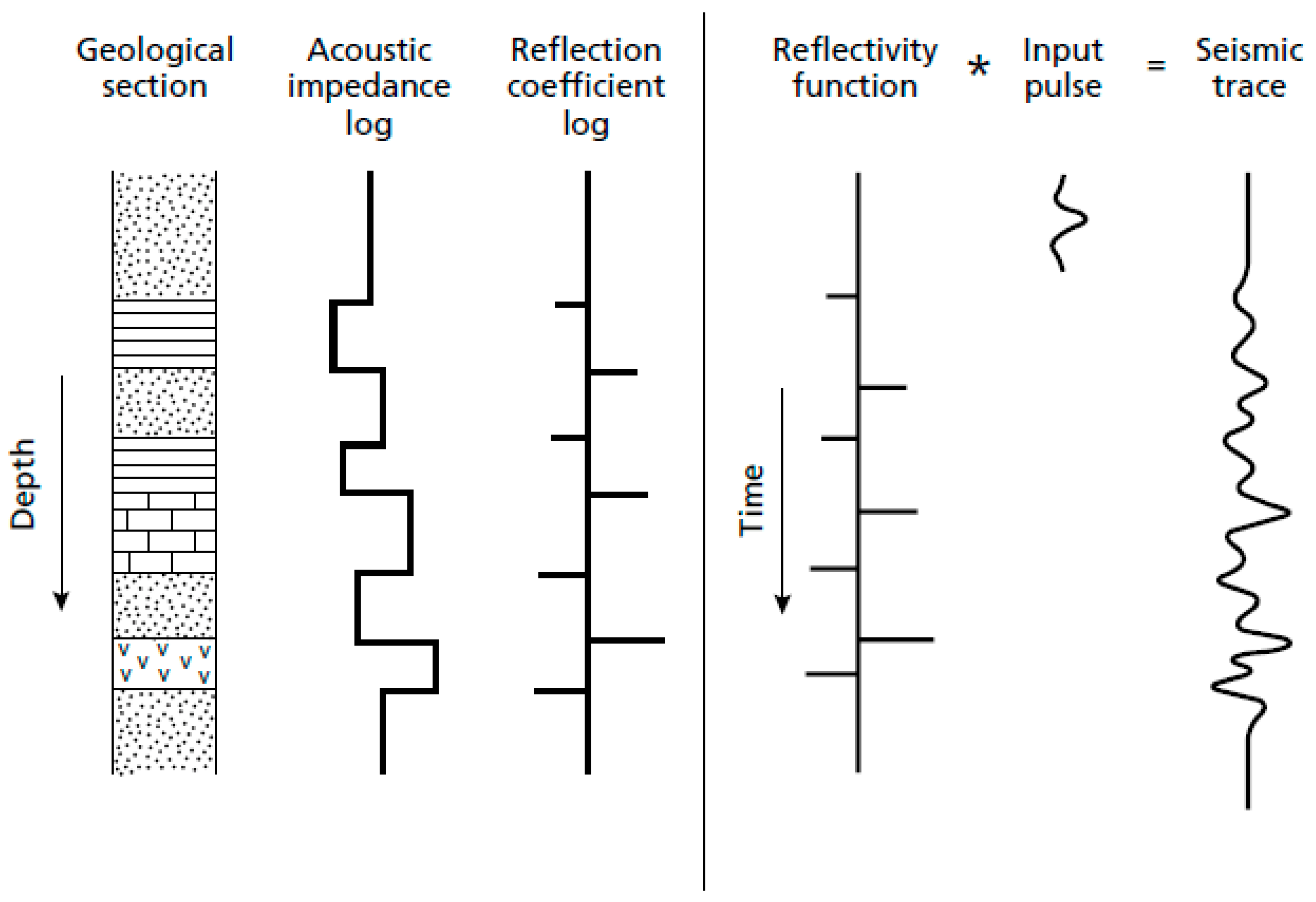
  41. Robinson, E.A. Seismic time-invariant convolutional model. Geophysics 1985, 50, 2297–2904. [Google Scholar] [CrossRef]
  42. Németh, K.; Frisch, W.; Meschede, M.; Blakey, R.C. Plate tectonics—Continental drift and mountain building. Bull. Volcanol. 2012, 74, 305–307. [Google Scholar] [CrossRef]
  43. Nanda, C.N. Seismic Data Interpretation and Evaluation for Hydrocarbon Exploration and Production; AOGEP Book Series; Springer: Cham, Switzerland, 2021; pp. 25–45. [Google Scholar]
  44. Maurya, S.P.; Singh, N.P.; Singh, K.H. Seismic Inversion Methods: A Practical Approach; Springer: Berlin/Heidelberg, Germany, 2020; pp. 1–18. [Google Scholar]
  45. Li, F.Q.; Ming, J.; Wei, T.G.; Xiong, Y.; Zhou, J.K. Application of the Matching Pursuit Based on Dipole Decomposition to Thin Reservoir of Bohai Bay Basin. In Proceedings of the 80th EAGE Conference and Exhibition 2018, Copenhagen, Denmark, 11–14 June 2018; Volume 2018, pp. 1–5. [Google Scholar]
  46. Ha, V. Application of Spectral Inversion to Enhance Seismic Resolution in Nam Con Son Basin, Offshore Vietnam. Master’s Thesis, University of Houston, Houston, TX, USA, 2014. Available online: https://uh-ir.tdl.org/bitstream/handle/10657/1674/HA-THESIS2014.pdf?sequence=1&isAllowed=y (accessed on 1 February 2021).
  47. Chakraborty, A.; Okaya, D. Frequency-time decomposition of seismic data using wavelet-based methods. Geophysics 1995, 60, 1906–1916. [Google Scholar] [CrossRef] [Green Version]
  48. Castagna, J.; Sun, S. Comparison of spectral decomposition methods. First Break 2006, 24, 75–79. [Google Scholar] [CrossRef]
  49. Puryear, C.I.; Portniaguine, O.N.; Cobos, C.M.; Castagna, J.P. Constrained least-squares spectral analysis: Application to seismic data. Geophysics 2012, 77, V143–V167. [Google Scholar] [CrossRef]
  50. Debeye, H.W.J.; van Riel, P. Lp-Norm Deconvolution. Geophys. Prospect. 1990, 38, 381–403. [Google Scholar] [CrossRef]
  51. Swain, S.; Jenamani, M.; Routray, A.; KumarSingh, S.; Tondon, R.; Bahuguna, C. PySLI: A software for Sparse Layer Inversion using Python. In Proceedings of the 13th Biennial International Concerence and Exhibition, Kochi, Japan, 23–25 February 2020. [Google Scholar]
  52. Margrave, G.F.; Lamoureux, M.P.; Henley, D.C. Gabor deconvolution: Estimating reflectivity by nonstationary deconvolution of seismic data. Geophysics 2011, 76, W15–W30. [Google Scholar] [CrossRef]
  53. Canales, L.L. Random Noise Reduction. SEG Ext. Abstr. 1984, 525–527. [Google Scholar] [CrossRef]
  54. Chaudhuri, A.K.; Deb, G.K. Proterozoic rifting in the Pranhita–Godavari Valley: Implication on India–Antarctica linkage. Gondwana Res. 2004, 7, 301–312. [Google Scholar] [CrossRef]
  55. Abma, R.; Claerbout, J. Lateral prediction for noise attenuation by t-x and F-X techniques. Geophysics 1995, 60, 1887–1896. [Google Scholar] [CrossRef] [Green Version]
  56. Yilmaz, O. Seismic Data Analysis: Processing, Inversion, and Interpretation of Seismic Data; Society of Exploration Geophysicists: Houston, TX, USA, 2001; ISBN 978-1-56080-099-6. [Google Scholar]
  57. Karsli, H. Further improvement of temporal resolution of seismic data by autoregressive (AR) spectral extrapolation. J. Appl. Geophys. 2006, 59, 324–336. [Google Scholar] [CrossRef]
  58. Rekapalli, R.; Tiwari, R.K.; Dhanam, K.; Seshunarayana, T. T-x frequency filtering of high resolution seismic reflection data using singular spectral analysis. J. Appl. Geophys. 2014, 105, 180–184. [Google Scholar] [CrossRef]
  59. Mirza, N.A.; Philip, R. Application of spectral decomposition and seismic attributes to understand the structure and distribution of sand reservoirs within Tertiary rift basins of the Gulf of Thailand: Interpreter’s Corner. Lead. Edge 2012, 31, 630–634. [Google Scholar]
  60. Butorin, A.V.; Krasnov, F.V.; GazpromneftScience & Technology Centre LLC. Spectral inversion methods and its application for wave field analysis. In Proceedings of the SPE Russian Petroleum Technology Conference, Moscow, Russia, 16–18 October 2017; pp. 1–12. [Google Scholar] [CrossRef]
  61. Taner, M.T.; Koehler, F.; Sheriff, R.E. Complex seismic trace analysis. Geophysics 1979, 44, 1041–1063. [Google Scholar] [CrossRef]
  62. Ansari, H.; Trusler, M.; Maitland, G.; Piane, C.D.; Pini, R. The gas-in-place and CO2 storage capacity of shale reservoirs at subsurface conditions. In Proceedings of the 15th Greenhouse Gas Control Technologies Conference, Online, 15–18 March 2021. [Google Scholar]
  63. Ridwan, T.K.; Hermana, M.; Lubis, L.A.; Riyadi, Z.A. New avo attributes and their applications for facies and hydrocarbon prediction: A case study from the northern malay basin. Appl. Sci. 2020, 10, 7786. [Google Scholar] [CrossRef]
  64. Ngui, J.Q.; Hermana, M.; Ghosh, D.; Yusof, W.I.W. Integrated study of lithofacies identification—A case study in X field, Sabah, Malaysia. Geosciences 2018, 8, 75. [Google Scholar] [CrossRef] [Green Version]
  65. Hermana, M.; Sani, M.N.M.; Harith, Z.Z.T.; Sum, C.W. Lithology Discrimination in Elastic Impedance Domain Using Artificial Neural Network. J. Eng. Technol. 2012, 2, 78–81. [Google Scholar]
Figure 1. Synthetic seismic response of a theoretical wedge model, (a) wedge and seismic traces, (b) amplitude extracted from top/base seismic marker (red) and measured through to peak time distance (green).
Applsci 12 05453 g001
Figure 2. Location map of Malay and other bounding basins (modified after [38]).
Applsci 12 05453 g002
Figure 3. Schematic geologic cross-section, showing the sequence stratigraphic Groups and geologic structures of Malay Basin (redrawn by [39], after [40]).
Applsci 12 05453 g003
Figure 4. Seismic base map showing the well locations.
Applsci 12 05453 g004
Figure 5. Schematic illustration of the convolutional model.
Applsci 12 05453 g005
Figure 6. A two-layer reflectivity model.
Applsci 12 05453 g006
Figure 7. Locating the analysis point at the center of the layer (red horizontal line).
Applsci 12 05453 g007
Figure 8. Any arbitrary pair of reflection coefficients r1 and r2 (Figure 7) can be represented as the sum of even and odd components. The even pair has equal magnitude and sign, and the odd pair has equal magnitude and opposite sign. The even and odd pair can be further decomposed into unit even and odd pairs respectively.
Applsci 12 05453 g008
Figure 9. Reflectivity amplitude spectrum for a simple layer of 50 ms thickness, with equal and opposite reflection coefficients of unit amplitude at the top and base. Modified after [19].
Applsci 12 05453 g009
Figure 10. Algorithmic scheme of the applied techniques.
Applsci 12 05453 g010
Figure 11. A plot of the original model parameter.
Applsci 12 05453 g011
Figure 12. A plot of the bandwidth-enhanced seismic trace model parameter showing an improved resolution after harmonic extrapolation was applied to the original spectrum.
Applsci 12 05453 g012
Figure 13. Comparison between the enhanced and original trace model.
Applsci 12 05453 g013
Figure 14. (a) Data spectrum of the enhanced trace model (b) and spectrum of the original trace model.
Applsci 12 05453 g014
Figure 15. Comparing the original (a) and the spectrally inverted (and harmonically extrapolated) filtered traces (b); (c) illustrates a comparison between the original trace with the enhanced trace.
Applsci 12 05453 g015
Figure 16. Comparison of the seismic traces (original and enhanced) with the reflectivity (RC) series from well data.
Applsci 12 05453 g016
Figure 17. Inas Field seismic data spectrum showing the original and enhanced spectral bandwidths.
Applsci 12 05453 g017
Figure 18. Comparison of the original (Track 3) and enhanced (Track 2) traces to the synthetic seismogram (Track 1). Track 3 shows an overlay of both traces. The horizontal black lines are the formation (correlation) tops across the synthetic and traces, and they match the seismic traces in time.
Applsci 12 05453 g018
Figure 19. A section of the original seismic volume at dip line—5215 (a) and a section through the improved seismic volume at dip line—5215 (b). The resolution of the enhanced volume is visibly improved and captures more geologic details when compared to the original data.
Applsci 12 05453 g019
Figure 20. Sections from seismic data showing the difference between bandlimited and enhanced data. (A) bandlimited data, (B) enhanced data.
Applsci 12 05453 g020
Figure 21. (a) generalized spectral decomposition of the data before bandwidth extrapolation (time slice—300 ms), (b) generalized spectral decomposition of the data after bandwidth extrapolation (time slice—300 ms). GSD volumes of 10, 30, and 40 Hz frequencies were blended using the RGB tool. The symbols ⊕ indicate the well locations.
Applsci 12 05453 g021
Publisher’s Note: MDPI stays neutral with regard to jurisdictional claims in published maps and institutional affiliations.

